Magnetic field induced chiral particle-hole condensates

Abstract

We demonstrate that a chiral particle-hole condensate is always induced by a number-conserving ground state of non-zero angular momentum in the presence of a magnetic field. The magnetic interaction originates from the coupling with the intrinsic orbital moment of the chiral state when the field is applied perpendicularly to the plane. According to our numerical results the induction mechanism is practically temperature independent providing robustness to these states up to high temperatures. This opens the door for manipulating the anomalous Hall response resulting from this intricate class of states for technological applications while it also suggests that chiral particle-hole condensates may be hidden in various complex materials.

Among the numerous states that emerge in a strongly correlated system in the particle-hole channel, the chiral states enjoy special attention. These states apart from the related symmetry breaking they effect due to the corresponding pair condensation, they additionally violate parity and time-reversal because of their special momentum structure (See e.g. Volovik ). As a consequence, the condensate carries an orbital moment that can be viewed as the effect of a non-zero Berry curvature in $\bm{k}$-space Berry ; LuttingerFerromagnetics ; semiclassical . The arising orbital moment OrbitalMagnetization provides the system with a magnetic field coupling leading to anomalous Hall transport and enhanced diamagnetic response. As a matter of fact, such states have ideal properties for technological applications. In addition the well established belief that unconventional particle-hole condensates are hidden in the majority of several important materials render these states as strong candidates for a pleiad of unidentified phases. Consequently, it is of high priority to be in position to generate these states and manipulate them, at our own disposal.

One of the traditional ways to controllably engineer novel states of matter is via applying an external field. Typical examples of field induced states in the area of particle-hole condensates constitute the field induced charge and spin density waves. There are several kinds of field induced density waves such as those occurring in organic quasi-1D conductors FISDW or even confined spin density waves GV both generated due to the orbital coupling with the magnetic field. Nevertheless, one may also obtain induced density waves driven by the Zeeman coupling aperis .

In this letter we perform a numerical study of the magnetic field induced planar chiral particle-hole condensates. A similar situation was first addressed by R. B. Laughlin Laughlin in the context of chiral d-wave superconductors to explain the magnetic field induced transition observed in Bi₂Sr₂CaCu₂O₈, and later extended to the particle-hole channel by J.-X. Zhu et al Balatsky . Since the whole class of these chiral states are characterized by a universal behaviour we shall concentrate on a particular state belonging to this class, the chiral d-density wave state, that recently attracted a lot of attention due to its prominent role in explaining the pseudogap regime of the cuprates Tewari ; KVL ; Meissner ; Zhang ; Spin ; Partha . By taking into account the effect of an external perpendicular magnetic field through its coupling with the intrinsic orbital magnetic moment of this state, we demonstrate through a detailed numerical analysis that a chiral state is necessarily induced or it is strongly enhanced if it already exists. In addition, we extract the magnetic field dependence of the two density wave order parameters, which is different in the above two cases. However, the interplay of the underlying interaction and the field strength can lead to a crossover in the magnetic field dependence in the latter case. Furthermore, we observe that the chiral d-density wave is robust against the increase of temperature in the presence of the external magnetic field, a direct consequence of the field driven enhancement. Our results are striking demonstrating that in many materials in which possibly only some components of a chiral particle-hole condensate develop, there will be unavoidably an induction of the rest and a concomitant transition to the complete chiral state in the presence of an external field, giving rise to the aforementioned intriguing response.

As we have already mentioned, the representative chiral particle-hole condensate that we shall consider is the chiral d-density wave state that constitutes a singlet unconventional density wave with a planar momentum structure, characterized by the commensurate wave-vector $\bm{Q}=(\pi/a,\pi/a)$. It is composed by a real $d_{xy}$ charge density wave violating parity and an imaginary $d_{x^{2}-y^{2}}$ orbital anti-ferromagnetic state giving rise to local charge currents and zero charge density, violating time-reversal. This state has been shown to exhibit unconventional Hall transport and anomalous magnetic response which is common to any other chiral particle-hole condensate with zero SCZ or finite momentum taking place either in the singlet or triplet channel of some kind of a spin degree of freedom, that is characterized by the same Berry curvature.

First of all, the chiral d-density wave is known to give rise to the Spontaneous Quantum Hall effect KVL ; Yakovenko , which concerns the generation of a quantized Hall voltage via the sole application of an electric field. Quite similarly, a thermoelectric Hall effect can be reproduced by the application of a finite temperature gradient Zhang . Moreover, this state supports topological spin transport characterized by dissipationless spin currents in the presence of a Zeeman field gradient Spin . An even more striking behaviour dominates the magnetic response of this system. The existence of the intrinsic orbital magnetic moment leads to perfect diamagnetism and consequently to the Topological Meissner effect demonstrated in Ref.Meissner . In the half-filled case the topological Meissner effect is identical to the usual superconducting diamagnetism, and motivated by this feature the chiral d-density wave state has been proposed to be hidden in the pseudogap phase of the cuprates. Furthermore, the observed Polar Kerr effect in YBa₂Cu₃O_6+x Xia , has been considered as a sharp signature of the chiral d-density wave state in underdoped cuprates Tewari .

To model the chiral d-density wave state we consider the following Hamiltonian

$${\cal H} = \sum_{\bm{k}}\left\{\varepsilon(\bm{k})c_{\bm{k}}^{{\dagger}}c_{\bm{k}}^{\phantom{{\dagger}}}+\varepsilon(\bm{k+Q})c_{\bm{k+Q}}^{{\dagger}}c_{\bm{k+Q}}^{\phantom{{\dagger}}}\right\}$$ (1)

$$- \frac{1}{v}\sum_{\bm{k},\bm{k}^{\prime}}{\cal V}(\bm{k},\bm{k}^{\prime})c_{\bm{k}}^{{\dagger}}c_{\bm{k}+\bm{Q}}^{\phantom{{\dagger}}}c_{\bm{k}^{\prime}+\bm{Q}}^{{\dagger}}c_{\bm{k}^{\prime}}^{\phantom{{\dagger}}}\,,$$

where we have introduced the single band energy dispersion of the free Bloch electrons $\varepsilon(\bm{k})=-2t[\cos(k_{x}a)+\cos(k_{y}a)]$ arising from the nearest neighbours hopping term and a 4-fermion interaction driven by an effective separable potential ${\cal V}(\bm{k},\bm{k}^{\prime})=V_{1}f_{1}(\bm{k})f_{1}(\bm{k}^{\prime})+V_{2}f_{2}(\bm{k})f_{2}(\bm{k}^{\prime})$, projecting only onto the form factors $f_{1}=\sin(k_{x}a)\sin(k_{y}a)$ and $f_{2}=\cos(k_{x}a)-\cos(k_{y}a)$ of the $d_{xy}$ and $d_{x^{2}-y^{2}}$ momentum space orbitals. The operators $c_{\bm{k}}^{\phantom{{\dagger}}}/c_{\bm{k}}^{{\dagger}}$ annihilate/create an electron of momentum $\bm{k}$ in the reduced Brillouin zone (R.B.Z.), $v$ is the volume of the system and $a$ the square lattice constant. For convenience we have omitted the spin indices, as we are dealing with a spin singlet state. Within a mean field decoupling we obtain the order parameter of the chiral d-density wave state $\Delta(\bm{k})=\Delta_{1}\sin(k_{x}a)\sin(k_{y}a)-i\Delta_{2}[\cos(k_{x}a)-\cos(k_{y}a)]$, which satisfies the self-consistence equation

$$\Delta(\bm{k})=-\frac{1}{v}\sum_{\bm{k}^{\prime}}{\cal V}(\bm{k},\bm{k}^{\prime})\left<c_{\bm{k}^{\prime}}^{{\dagger}}c_{\bm{k}^{\prime}+\bm{Q}}^{\phantom{{\dagger}}}\right>\,,$$ (2)

with $<>$ denoting thermal and quantum-mechanical average. For convenience, we adopt a more compact notation by considering the enlarged spinor $\Psi_{\bm{k}}^{{\dagger}}=(c_{\bm{k}}^{{\dagger}}\phantom{{\dagger}}c_{\bm{k+Q}}^{{\dagger}})$ and employing the $\bm{\tau}$ Pauli matrices. The mean field Hamiltonian now becomes ${\cal H}=\sum_{\bm{k}}\Psi_{\bm{k}}^{{\dagger}}{\cal H}(\bm{k})\Psi_{\bm{k}}^{\phantom{{\dagger}}}=\sum_{\bm{k}}\Psi_{\bm{k}}^{{\dagger}}\phantom{.}\bm{g}(\bm{k})\cdot\bm{\tau}\phantom{.}\Psi_{\bm{k}}^{\phantom{{\dagger}}}$ where we have introduced the isovector $\bm{g}(\bm{k})$ defined as $\bm{g}(\bm{k})=\left({\cal R}e\Delta(\bm{k}),-{\cal I}m\Delta(\bm{k}),\varepsilon(\bm{k})\right)$. The one-particle Hamitonian for each $\bm{k}$-mode is a $2\times 2$ matrix

$${\cal H}(\bm{k})=\left(\begin{array}[]{cc}g_{3}^{\phantom{{\dagger}}}(\bm{k})&g_{1}^{\phantom{{\dagger}}}(\bm{k})-ig_{2}^{\phantom{{\dagger}}}(\bm{k})\\ g_{1}^{\phantom{{\dagger}}}(\bm{k})+ig_{2}^{\phantom{{\dagger}}}(\bm{k})&-g_{3}^{\phantom{{\dagger}}}(\bm{k})\\ \end{array}\right)\,.$$ (5)

To incorporate the interaction with the magnetic field we shall consider only the orbital coupling and neglect the Zeeman term as it is usually negligible in the case we are considering. To calculate the orbital moment one has to determine the Berry phase emerging in this chiral state when $\bm{k}$ changes adiabatically along a closed loop. For instance, the variation of $\bm{k}$ can be enforced by the minimal coupling $\bm{k}\rightarrow\bm{k}-e\bm{{\cal E}}t$ if we apply a constant electric field $\bm{{\cal E}}$. In this case, the Hamiltonian becomes parametric ${\cal H}(\bm{k})\rightarrow{\cal H}(\bm{k},t)$. Within the adiabatic approximation, the emerging Berry phase can be determined using the instantaneous (snapshot) eigenstates of the parametric Hamiltonian $|\Phi_{\nu}(\bm{k},t)$, satisfying ${\cal H}(\bm{k},t)|\Phi_{\nu}(\bm{k},t)\rangle=E_{\nu}(\bm{k},t)|\Phi_{\nu}(\bm{k},t)\rangle$. In this equation, $t$, is introduced only as a parameter. This means that these snapshot eigenstates are not really time-dependent but only parameter dependent, which in our case coincides with $t$. Our two band system, is characterized by the snapshot eigenstates $|\Phi_{\pm}\rangle$ and the corresponding eigenenergies $E_{\pm}(\bm{k},t)=\pm|g(\bm{k},t)|$. By defining $g_{1}^{\phantom{{\dagger}}}(\bm{k})=E(\bm{k})\sin\theta(\bm{k})\cos\varphi(\bm{k})$, $g_{2}^{\phantom{{\dagger}}}(\bm{k})=E(\bm{k})\sin\theta(\bm{k})\sin\varphi(\bm{k})$ and $g_{3}^{\phantom{{\dagger}}}(\bm{k})=E(\bm{k})\cos\theta(\bm{k})$, we obtain a convenient expression for the snapshot eigenstates of the system

$$|\Phi_{+}^{\phantom{{\dagger}}}(\bm{k},t)\rangle=\left(\begin{array}[]{l}\cos\left(\frac{\theta(\bm{k},t)}{2}\right),\phantom{-}\sin\left(\frac{\theta(\bm{k},t)}{2}\right)e^{i\varphi(\bm{k},t)}\end{array}\right)^{T},$$ (7)

$$|\Phi_{-}^{\phantom{{\dagger}}}(\bm{k},t)\rangle=\left(\begin{array}[]{l}\sin\left(\frac{\theta(\bm{k},t)}{2}\right),-\cos\left(\frac{\theta(\bm{k},t)}{2}\right)e^{i\varphi(\bm{k},t)}\end{array}\right)^{T}\,,$$ (9)

with $E(\bm{k})=|g(\bm{k})|$ and ^T denoting matrix transposition. The orbital magnetic moment $\bm{m}_{\nu}^{\phantom{{\dagger}}}(\bm{k})$ is determined by the relation $\bm{m}_{\nu}^{\phantom{{\dagger}}}(\bm{k})=\frac{e}{2\hbar i}\langle\bm{\nabla}_{\bm{k}}^{\phantom{{\dagger}}}\Phi_{\nu}^{\phantom{{\dagger}}}(\bm{k})\mid\times\left[{\cal H}(\bm{k})-E_{\nu}^{\phantom{{\dagger}}}(\bm{k})\right]\mid\bm{\nabla}_{\bm{k}}^{\phantom{{\dagger}}}\Phi_{\nu}^{\phantom{{\dagger}}}(\bm{k})\rangle=\frac{e\nu}{\hbar}E(\bm{k})\bm{\Omega}_{\nu}^{\phantom{{\dagger}}}(\bm{k})$ where we have introduced the Berry curvature Spin

$$\bm{\Omega}_{\nu}^{\phantom{{\dagger}}}(\bm{k})=-\frac{\nu}{2E^{3}(\bm{k})}\phantom{.}\bm{g}(\bm{k})\cdot\left(\frac{\partial\bm{g}(\bm{k})}{\partial k_{x}^{\phantom{{\dagger}}}}\times\frac{\partial\bm{g}(\bm{k})}{\partial k_{y}^{\phantom{{\dagger}}}}\right)=\Omega^{z}_{\nu}\phantom{.}\bm{\hat{z}}.\,$$ (10)

We notice the Berry curvature and the orbital moment lie along the $z$-axis, as a direct consequence of the planar character of our system. The presence of a perpendicular magnetic field $\bm{{\cal B}}$ enters the band dispersions of the system in the following way $E_{\nu}^{\bm{{\cal B}}}(\bm{k})=E_{\nu}^{\phantom{{\dagger}}}(\bm{k})-\bm{m}_{\nu}^{\phantom{{\dagger}}}(\bm{k})\cdot\bm{{\cal B}}$.

Having obtained the energy dispersions of the system in presence of the magnetic field we may now extract the self-consistence equations of the $d_{xy}$ and $d_{x^{2}-y^{2}}$ order parameters $\Delta_{1},\Delta_{2}$. The free energy functional is defined as OrbitalMagnetization

$${\cal F}=\frac{\Delta^{2}_{1}}{V_{1}^{\phantom{{\dagger}}}}+\frac{\Delta^{2}_{2}}{V_{2}^{\phantom{{\dagger}}}}-\frac{1}{v\beta}\sum_{\bm{k},\nu=\pm}Ln\left(1+e^{-\beta E_{\nu}^{\bm{{\cal B}}}(\bm{k})}\right)\phantom{.}\,.$$ (11)

with $\beta=1/k_{B}^{\phantom{{\dagger}}}T$. The first two terms in the free energy originate from the mean field decoupling and correspond to the elastic energy waisted for building up the two density wave gaps. Minimization of this functional with respect to the order parameter doublet leads to the following system of coupled self-consistence equations

$$\frac{\partial{\cal F}}{\partial\Delta_{i}^{\phantom{{\dagger}}}}=0\Rightarrow\Delta_{i}^{\phantom{{\dagger}}}=\frac{2}{v}\sum_{\bm{k},\nu}\left\{-V_{i}^{\phantom{{\dagger}}}\Delta_{i}^{\phantom{{\dagger}}}\frac{f_{i}^{2}(\bm{k})}{2E(\bm{k})}\nu+\frac{ea^{2}t}{\hbar}{\cal B}_{z}^{\phantom{{\dagger}}}V_{i}^{\phantom{{\dagger}}}\widetilde{\Delta}_{i}^{\phantom{{\dagger}}}\frac{s(\bm{k})}{E^{2}(\bm{k})}\left[1-2\left(\frac{\Delta_{i}^{\phantom{{\dagger}}}(\bm{k})}{E(\bm{k})}\right)^{2}\right]\right\}n_{F}^{\phantom{{\dagger}}}\left[E_{\nu}^{\bm{{\cal B}}}(\bm{k})\right],\phantom{{\dagger}}i=1,2\,,$$ (12)

that will be used for determining the chiral d-density wave gaps numerically. In the above, we have introduced $s(\bm{k})=\sin^{2}(k_{x}a)\cos^{2}(k_{y}a)+\sin^{2}(k_{y}a)$, $\widetilde{\Delta}_{1,2}=\Delta_{2,1}$, $n_{F}^{\phantom{{\dagger}}}(E)$ the Fermi-Dirac distribution and multiplied by a factor of two in order to take into account the electron spin. The first term corresponds to the equation that we obtain in a zero magnetic field with the only difference that the energy bands $E_{\nu}^{\phantom{{\dagger}}}$ are shifted by the orbital coupling $-\bm{m}_{\nu}^{\phantom{{\dagger}}}\cdot\bm{{\cal B}}$. On the other hand, the second term is attributed entirely to the magnetic field interaction with the chiral d-density wave state. As a matter of fact, it is the essential ingredient for a field induced chiral d-density wave. To understand how a magnetic field stabilizes this chiral state we consider the case of $\Delta_{1}=0$ and $\Delta_{2}\neq 0$. In this case the initial state is an orbital anti-ferromagnet. We may calculate the induced $\Delta_{1}$ component by setting $\Delta_{1}=0$ on the right hand side of Eq.(12). It is straightforward to obtain that $\Delta_{1}^{induced}=\frac{ea^{2}t}{\hbar}{\cal B}_{z}^{\phantom{{\dagger}}}V_{2}^{\phantom{{\dagger}}}\Delta_{2}^{\phantom{{\dagger}}}{\cal I}({\cal B}_{z}^{\phantom{{\dagger}}})$ with ${\cal I}({\cal B}_{z}^{\phantom{{\dagger}}})$ corresponding to a suitable sum over R.B.Z. of the remaining terms. Apart from the additional weak dependence on the field in ${\cal I}$, this formula also agrees with the one derived in Ref.Balatsky using a different method. According to our result a chiral d-density wave state is always generated even for an arbitrary small magnetic field.

We now proceed in solving numerically the system of self-consistence equations. For all our numerical simulations we set $t=250$meV, $a=5$Å and $V_{2}=150$meV. The last condition aims to establish a $d_{x^{2}-y^{2}}$ density wave of approximately a $\Delta_{2}\simeq 53$meV gap for all the possible temperatures and magnetic fields considered here. The latter consideration helps us to focus solely on the behaviour of the $d_{xy}$ component. For the calculations we have set up an $128\times 128$ grid in the right upper quadrant of the Brillouin zone. A large number of points are needed in order to stabilize a value for the $d_{xy}$ order parameter.

First of all, we verify numerically the linear dependence on the magnetic field of the induced $d_{xy}$ order parameter. For the illustration we consider $V_{1}=125$meV, a value that in zero magnetic field would provide a practically zero $d_{xy}$ gap. In the inset of Fig.1 we do observe the expected linear scaling while we also notice the extremely weak temperature dependence. The latter is attributed to the manner in which the Fermi-Dirac occupation numbers enter the second part of the self-consistence equations. Specifically, the occupation numbers of the two bands add up giving $n_{F}^{\phantom{{\dagger}}}\left[-E(\bm{k})-m_{z}^{\phantom{{\dagger}}}(\bm{k}){\cal B}_{z}^{\phantom{{\dagger}}}\right]+n_{F}^{\phantom{{\dagger}}}\left[E(\bm{k})-m_{z}^{\phantom{{\dagger}}}(\bm{k}){\cal B}_{z}^{\phantom{{\dagger}}}\right]\simeq 1$ due to the negligibleness of the magnetic coupling compared to $E(\bm{k})$.

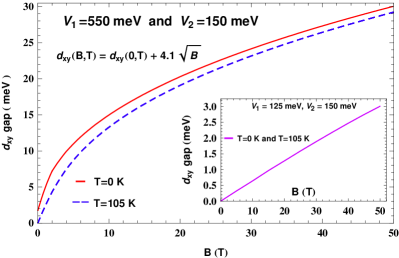
Figure 1: (Color online) Magnetic field induced chiral d-density wave. In the inset, we present the magnetic field dependence of the induced $d_{xy}$ component when only a $d_{x^{2}-y^{2}}$ already exists, for two different temperatures. In the main panel we demonstrate the strengthening due to the field, of an initially subdominant $d_{xy}$ component of a preexisting chiral d-density wave state. The two curves presented for the $d_{xy}$ part differ only on the zero field gap value arising from the usual BCS temperature dependence. As we may observe, the induced part of the chiral state is always temperature insensitive, while the field dependence changes from linear to square root.

More intriguing results emerge in the case of an initially existing chiral d-density wave state. We consider the combination of potentials $V_{1}=550$meV and $V_{2}=150$meV, generating the gaps $\Delta_{1}\simeq 1.8$meV and $\Delta_{2}\simeq 53$meV in the absence of the field. When the orbital magnetic coupling is switched on, the $d_{x^{2}-y^{2}}$ gap remains mostly unaffected while the $d_{xy}$ component is significantly enhanced. Specifically, the magnitude of the gap becomes about $15$ times bigger for ${\cal B}_{z}^{\phantom{{\dagger}}}$=50T. Moreover, we observe that the magnetic field dependence of the latter gap turns out to be square root contrary to the linear dependence obtained earlier. Of course, this difference arises from the first term of the self-consistence equation which dominates the zero field limit and is fully active here, compared to the previous situation.

As far as the temperature dependence is concerned, we notice in the main panel of Fig.1 that for two totally different temperature regimes we only have a shift of the two curves, equal to the difference of the $d_{xy}$ gap value obtained in these temperatures in the absence of the field. Apparently, the induced part of the $d_{xy}$ gap is once again temperature independent as it originates solely from the magnetic field coupling term. We also obtain the temperature evolution for different magnetic field values. For example a $\Delta_{1}=1.8$meV gap initially disappearing at about $30$K is now robust over a temperature range of more than $120$K. This is natural if we take into account that the magnetic field has strengthened the zero temperature gap of the order parameter that would now collapse to a higher temperature following the usual BCS behaviour.

Finally, we examine the influence of the $d_{xy}$ interaction potential, on the corresponding gap magnetic field dependence. Fig.2 shows the field dependence of the $d_{xy}$ gaps for several potentials after subtracting the zero field contribution. Focusing on the induced part of the gap we conclude that the increase of the interaction strength softens the square root field dependence turning it into a linear one. This crossover behaviour is indicative of the enhancement of the magnetic field coupling that favours a linear trend. As a matter of fact, this features serve as a potential diagnostic method for the interaction energy scale.

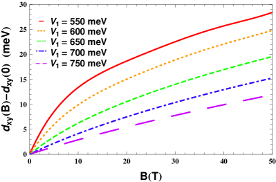
Figure 2: (Color online) Magnetic field dependence of the induced part of the $d_{xy}$ component in a preexisting chiral d-density wave state for several interaction potentials. For small values of the potential we obtain the expected square root behaviour, while after a critical value a crossover to a linear dependence is triggered. The latter, signals the dominance of the magnetic field coupling over the zero field 4-fermion $d_{xy}$-channel interaction strength. (For the calculations we have used $V_{2}$=150meV.)

In conclusion, we have studied numerically the occurrence of magnetic field induced chiral particle-hole condensates due to the coupling of their intrinsic orbital moment to a perpendicular magnetic field. According to our results, if an incomplete chiral state develops in zero field, such as a $d_{x^{2}-y^{2}}$ density wave, then a $d_{xy}$ is generated spontaneously when the magnetic interaction is triggered. The magnetic field dependence of the $d_{xy}$ gap is linear. On the other hand, if a small $d_{xy}$ compared to the $d_{x^{2}-y^{2}}$ already exists, then it will have a square root dependence on the magnetic field that can become linear if the interaction potential in the $d_{xy}$ channel exceeds a critical value. In both cases we obtain a negligible dependence of the induced order parameters on temperature. Consequently, chiral particle-hole condensates can survive up to high temperatures as long as the magnetic coupling persists.

The unavoidable transition to a chiral state has strong impact on materials that are proposed to host orbital anti-ferromagnetic states. For instance, the well established d-density wave scenario Chakravarty in the pseudogap regime of the cuprates provides a unique occasion for the realization of a chiral state, the chiral d-density wave. In this case, its presence is ensured when an external perpendicular field is applied but it could also be present in zero field if the necessary orbital interaction originates from intrinsic sources such as magnetic impurities.

We are grateful to A. Aperis and S. Kourtis for enlightening discussions on numerical methods. Moreover, P.K. is indebted to Professor C. Panagopoulos and Partha Goswami for valuable comments and suggestions. One of the authors (P.K.) acknowledges financial support by the Greek National Technical University Scholarships Foundation.

References

- (1) G. E. Volovik, The Universe in a Helium Droplet, Oxford Science Publications (2003).
- (2) M.V. Berry, Proc. R. Soc. London A 392, 45 (1984); R. Resta, Rev. of Mod. Phys. 66, 899 (1994).
- (3) M.-C. Chang and Q. Niu, Phys. Rev. B 53, 7010 (1996); G. Sundaram and Q. Niu, Phys. Rev. B 59, 14915 (1999).
- (4) R. Karplus and J.M. Luttinger, Phys. Rev. 95, 1154 (1954); J.M. Luttinger, Phys. Rev. 112, 739 (1958); T. Jungwirth, Q. Niu, and A. H. MacDonald, Phys. Rev. Lett. 88, 207208 (2002); M. Onoda and N. Nagaosa, J. Phys. Soc. Jpn. 71, 19 (2002).
- (5) J. Shi, G. Vignale, D. Xiao and Q. Niu, Phys. Rev. Lett. 99, 197202 (2007); T. Thonhauser, D. Ceresoli, D. Vanderbilt, and R. Resta, Phys. Rev. Lett. 95, 137205 (2005).
- (6) L. P. Gorkov and A. G. Lebed , J. Phys. Lett. 45, L433 (1984); M. Héritier, G. Montambaux and P. Lederer, J. Phys. Lett. 45, L943 (1984); V. M. Yakovenko, Phys. Rev. B. 43, 11353 (1991).
- (7) G. Varelogiannis and M. Héritier, J. Phys.: Condens. Matter 15, L673 (2003).
- (8) A. Aperis, M. Georgiou, G. Roumpos, S. Tsonis, G. Varelogiannis and P. B. Littlewood, Europhys. Lett., 83, 67008 (2008).
- (9) R. B. Laughlin, Phys. Rev. Lett. 80, 5188 (1998)
- (10) Jian-Xin Zhu and A. V. Balatsky, Phys. Rev. B 65, 132502 (2002).
- (11) S. Tewari, C. Zhang, V. M. Yakovenko, and S. Das Sarma, Phys. Rev. Lett. 100, 217004 (2008).
- (12) P. Kotetes and G. Varelogiannis, Europhys. Lett., 84, 37012 (2008).
- (13) P. Kotetes and G. Varelogiannis, Phys. Rev. B., 78, 220509(R) (2008).
- (14) C. Zhang, S. Tewari, V. M. Yakovenko, and S. Das Sarma, Phys. Rev. B., 78, 174508 (2008).
- (15) P. Kotetes and G. Varelogiannis, J. Supercond. Nov. Magn., 22, 141-145 (2009).
- (16) P. Goswami, arXiv:0905.1533.
- (17) K. Sun and E. Fradkin, Phys. Rev. B. 78, 245122 (2008); C. Wu, K. Sun, E. Fradkin, and S.-C. Zhang, Phys. Rev. B. 75, 115103 (2007).
- (18) V. M. Yakovenko, Phys. Rev. Lett. 65, 251 (1990).
- (19) J. Xia, E. Schemm, G. Deutscher, S. A. Kivelson, D. A. Bonn, W. N. Hardy, R. Liang, W. Siemons, G. Koster, M. M. Fejer, and A. Kapitulnik, Phys. Rev. Lett. 100, 127002 (2008).
- (20) S. Chakravarty, R. B. Laughlin, D. K. Morr, and C. Nayak, Phys. Rev. B 63, 094503 (2001).