Entanglement of coupled massive scalar field in background of dilaton black hole

Abstract

The entanglement of the coupled massive scalar field in the spacetime of a Garfinkle-Horowitz-Strominger(GHS) dilaton black hole has been investigated. It is found that the entanglement does not depend on the mass of the particle and the coupling between the scalar field and the gravitational field, but it decreases as the dilaton parameter $D$ increases. It is interesting to note that in the limit of $D\rightarrow M$, corresponding to the case of an extreme black hole, the state has no longer distillable entanglement for any state parameter $\alpha$, but the mutual information equals to a nonvanishing minimum value, which indicates that the total correlations consist of classical correlations plus bound entanglement in this limit.

I introduction

Quantum entanglement is both the central concept and the major resource in quantum information tasks such as quantum teleportation and quantum computation Peres ; Boschi ; Bouwmeester ; Pan . As relativistic field theory provides not only a more complete theoretical framework but also many experimental setups, relativistic quantum information theory may become an essential theory in the near future with possible applications to quantum entanglement and quantum teleportation. Thus, considerable effort has been expended on the investigation of quantum entanglement in the relativistic framework Peres ; Alsing-Milburn ; Ge-Kim ; Ling ; Adesso . It has been shown that for scalar and Dirac fields, the degradation of entanglement will occur from the perspective of a uniformly accelerated observer, which essentially originates from the fact that the event horizon appears and Unruh effect results in a loss of information for the non-inertial observer Schuller-Mann ; Alsing-Mann ; unruh ; Qiyuan ; Pan Qiyuan .

On the other hand, string theory with an extra space compactified at a larger length scale or lower energy scale than the Planck scale has been an attractive idea to solve the gauge hierarchy problem and possibly a candidate for quantum gravity arkani . There is also a growing interest in dilaton black holes from the string theory in the last few years. Meanwhile, it is generally believed that the study of quantum entanglement in the background of a dilaton black hole may lead to a deeper understanding of black holes and quantum gravity because it is related to the quantum information theory, string theory and loop quantum gravity Dreyer ; chen . In this paper, we will analyze the entanglement for the coupled massive scalar field in the spacetime of a GHS dilaton black hole, which was derived from the string theory. In particular, we here choose the generically entangled state $\sqrt{1-\alpha^{2}}|0\rangle_{A}|1\rangle_{B}+\alpha|1\rangle_{A}|0\rangle_{B}$ rather than the maximally entangled state $\frac{1}{\sqrt{2}}(|0\rangle_{A}|0\rangle_{B}+|1\rangle_{A}|1\rangle_{B})$ in an inertial reference frame. It seems to be an interesting study to consider the influences of the dilaton of the black hole, the mass of the particle and the coupling between the scalar field and the gravitational field on the quantum entangled states and show how they will change the properties of the entanglement. We assume that Alice has a detector which only detects mode $|n\rangle_{A}$ and Bob has a detector sensitive only to mode $|n\rangle_{B}$, and they share a generically entangled state at the same initial point in flat Minkowski spacetime before the black hole is formed. After the coincidence of Alice and Bob, Alice stays stationary at the asymptotically flat region, while the other observer, Bob, moves from the flat place toward the dilaton black hole. This won’t change the metric outside of the black hole and therefore won’t change Bob’s acceleration Birkhoff . Thus, Bob’s detector registers only thermally excited particles due to the Hawking effect unruh-1 .

The outline of this paper is as follows. In Sec. 2 we discuss vacuum structure of coupled massive scalar field in the spacetime. In Sec. 3 we analyze the effects of the dilaton parameter $D$, mass of the particle and the coupling between the scalar field and the gravitational field on the entanglement between the modes for the different state parameter $\alpha$. We summarize and discuss our conclusions in the last section.

II Vacuum structure of coupled massive scalar field

The metric for a GHS black hole spacetime can be expressed as Horowitz

$$ds^{2}=-\left(\frac{r-2M}{r-2D}\right)dt^{2}+\left(\frac{r-2M}{r-2D}\right)^{-1}dr^{2}+r(r-2D)d\Omega^{2},$$ (1)

where $M$ and $D$ are parameters related to mass of the black hole and dilaton field. The relationship among $M$, the charge $Q$ and $D$ is described as $D=Q^{2}/2M$. Throughout this paper we use $G=c=\hbar=\kappa_{B}=1$.

The general perturbation equation for a coupled massive scalar field in this dilaton spacetime is given by chen

$$\frac{1}{\sqrt{-g}}\partial_{\mu}(\sqrt{-g}g^{\mu\nu}\partial_{\nu})\psi-(\mu+\xi R)\psi=0,$$ (2)

where $\mu$ is the mass of the particle, $\psi$ is the scalar field and $R$ is the Ricci scalar curvature. The coupling between the scalar field and the gravitational field is represented by the term $\xi R\psi$, where $\xi$ is a numerical coupling factor. After expressing the normal mode solution as

$$\psi_{\omega lm}=\frac{1}{h(r)}\chi_{\omega l}(r)Y_{lm}(\theta,\varphi)e^{-i\omega t},$$ (3)

where $Y_{lm}(\theta,\varphi)$ is a scalar spherical harmonic on the unit twosphere and $h(r)=\sqrt{r(r-2D)}$, we can easily get the radial equation

$$\frac{d^{2}\chi_{\omega l}}{dr_{*}^{2}}+[\omega^{2}-V(r)]\chi_{\omega l}=0,$$ (4)

with

$$V(r)=\frac{f(r)}{h(r)}\frac{d}{dr}\left[f(r)\frac{dh(r)}{dr}\right]+\frac{f(r)l(l+1)}{h^{2}(r)}+f(r)\bigg{[}\mu^{2}+\frac{2\xi D^{2}(r-2M)}{r^{2}(r-2D)^{3}}\bigg{]},$$ (5)

where $dr_{*}=dr/f(r)$ is the tortoise coordinates and $f(r)=(r-2M)/(r-2D)$.

Solving Eq. (4) near the event horizon, we obtain the incoming mode which is analytic everywhere in the spacetime manifold

$$\phi_{in,\omega lm}=e^{-i\omega v}Y_{lm}(\theta,\varphi),$$ (6)

and the outgoing mode for the inside and outside region of the event horizon

$$\phi_{out,\omega lm}(r<r_{+})=e^{i\omega u}Y_{lm}(\theta,\varphi),$$ (7)

$$\phi_{out,\omega lm}(r>r_{+})=e^{-i\omega u}Y_{lm}(\theta,\varphi),$$ (8)

where $v=t+r_{*}$ and $u=t-r_{*}$. Eqs. (7) and (8) are analytic inside and outside the event horizon respectively, so they form a complete orthogonal family.

By defining the generalized light-like Kruskal coordinates Ge-Kim

$$u=-4(M-D)\ln[-U/(4M-4D)],\quad$$

$$v=4(M-D)\ln[V/(4M-4D)],\quad{\rm if\quad r>r_{+}};$$

$$u=-4(M-D)\ln[U/(4M-4D)],\quad$$

$$v=4(M-D)\ln[V/(4M-4D)],\quad{\rm if\quad r<r_{+}},$$ (9)

we can rewrite Eqs. (7) and (8) in the following form

$$\phi_{out,\omega lm}(r<r_{+})=e^{-4(M-D)i\omega\ln[-U/(4M-4D)]}Y_{lm}(\theta,\varphi),$$ (10)

$$\phi_{out,\omega lm}(r>r_{+})=e^{4(M-D)i\omega\ln[U/(4M-4D)]}Y_{lm}(\theta,\varphi).$$ (11)

By using the formula $-1=e^{i\pi}$ and making (10) analytic in the lower half-plane of $U$, we find a complete basis for positive energy $U$ modes

$$\phi_{I,\omega lm}=e^{2\pi\omega(M-D)}\phi_{out,\omega lm}(r>r_{+})+e^{-2\pi\omega(M-D)}\phi^{*}_{out,\omega lm}(r<r_{+}),$$ (12)

$$\phi_{II,\omega lm}=e^{-2\pi\omega(M-D)}\phi^{*}_{out,\omega lm}(r>r_{+})+e^{2\pi\omega(M-D)}\phi_{out,\omega lm}(r<r_{+}).$$ (13)

Eqs. (12) and (13) are complete basis for positive frequency modes which analytic for all real $U$ and $V$. Thus, we can also quantize the quantum field in terms of $\phi_{I,\omega lm}$ and $\phi_{II,\omega lm}$ in the Kruskal spacetime.

Using the second-quantizing the field in the exterior of this dilaton black hole Ge-Kim ; unruh ; Pan Qiyuan , we can obtain the Bogoliubov transformations for the particle annihilation and creation operators in the dilaton and Kruskal spacetime

$$a_{K,\omega lm}=\frac{b_{out,\omega lm}}{\sqrt{1-e^{-8\pi\omega(M-D)}}}-\frac{b^{{\dagger}}_{in,\omega lm}}{\sqrt{e^{8\pi\omega(M-D)}-1}},$$

$$a^{{\dagger}}_{K,\omega lm}=\frac{b^{{\dagger}}_{out,\omega lm}}{\sqrt{1-e^{-8\pi\omega(M-D)}}}-\frac{b_{in,\omega lm}}{\sqrt{e^{8\pi\omega(M-D)}-1}},$$ (14)

where $a_{K,\omega lm}$ and $a^{{\dagger}}_{K,\omega lm}$ are the annihilation and creation operators acting on the Kruskal vacuum of the exterior region, $b_{in,\omega lm}$ and $b^{{\dagger}}_{in,\omega lm}$ are the annihilation and creation operators acting on the vacuum of the interior region of the black hole, and $b_{out,\omega lm}$ and $b^{{\dagger}}_{out,\omega lm}$ are the annihilation and creation operators acting on the vacuum of the exterior region respectively.

Now the Kruskal vacuum $|0\rangle_{K}$ outside the event horizon is defined by

$$a_{K,\omega lm}|0\rangle_{K}=0.$$ (15)

After properly normalizing the state vector, we obtain the Kruskal vacuum which is a maximally entangled two-mode squeezed state Barnett ; Ahn

$$|0\rangle_{K}=\sqrt{1-e^{-8\pi\omega(M-D)}}\sum_{n=0}^{\infty}e^{-4n\pi\omega(M-D)}|n\rangle_{in}\otimes|n\rangle_{out},$$ (16)

and the first excited state

$$|1\rangle_{K}=a^{{\dagger}}_{K,\omega lm}|0\rangle_{K}$$

$$=[1-e^{-8\pi\omega(M-D)}]\sum_{n=0}^{\infty}\sqrt{n+1}~{}e^{-4n\pi\omega(M-D)}|n\rangle_{in}\otimes|n+1\rangle_{out},$$ (17)

where $\{|n\rangle_{in}\}$ and $\{|n\rangle_{out}\}$ are the orthonormal bases for the inside and outside region of the event horizon respectively. For the observer outside the black hole, he needs to trace over the modes in the interior region since he has no access to the information in this causally disconnected region. Thus, the Hawking radiation spectrum can be obtained by

$$N_{\omega}^{2}=_{K}\langle 0|b^{{\dagger}}_{K,\omega lm}b_{K,\omega lm}|0\rangle_{K}=\frac{1}{e^{8\pi\omega(M-D)}-1},$$ (18)

Eq. (18) shows that the observer in the exterior of the GHS dilaton black hole detects a thermal Bose-Einstein distribution of particles as he traverses the Kruskal vacuum.

III Quantum entanglement in background of GHS dilaton black hole

We will discuss quantum entanglement with the coupled massive scalar field in the GHS dilaton black hole spacetime. We assume that Alice has a detector which only detects mode $|n\rangle_{A}$ and Bob has a detector sensitive only to mode $|n\rangle_{B}$, and they share a generically entangled state at the same initial point in flat Minkowski spacetime before the black hole is formed. The initial entangled state is

$$|\Psi\rangle=\sqrt{1-\alpha^{2}}|0\rangle_{A}|1\rangle_{B}+\alpha|1\rangle_{A}|0\rangle_{B},$$ (19)

where $\alpha$ is some real number which satisfies $|\alpha|\in(0,1)$, $\alpha$ and $\sqrt{1-\alpha^{2}}$ are the so-called “normalized partners”. Using Eqs. (16) and (II), we can rewrite Eq. (19) in terms of Minkowski modes for Alice and black hole modes for Bob. Since Bob is causally disconnected from the interior region of the black hole, we will take the trace over the states in this region and obtain the mixed density matrix between Alice and Bob in the exterior region

$$\rho_{AB}=[1-e^{-8\pi\omega(M-D)}]\sum_{n=0}^{\infty}\rho_{n}~{}e^{-8n\pi\omega(M-D)},$$

$$\rho_{n}=\alpha^{2}|1n\rangle\langle 1n|+(n+1)(1-\alpha^{2})[1-e^{-8\pi\omega(M-D)}]|0(n+1)\rangle\langle 0(n+1)|$$

$$\qquad+\alpha\sqrt{(n+1)(1-\alpha^{2})[1-e^{-8\pi\omega(M-D)}]}|1n\rangle\langle 0(n+1)|$$

$$\qquad+\alpha\sqrt{(n+1)(1-\alpha^{2})[1-e^{-8\pi\omega(M-D)}]}|0(n+1)\rangle\langle 1n|,$$ (20)

where $|nm\rangle=|n\rangle_{A}|m\rangle_{B,out}$.

To determine whether this mixed state is entangled or not, we here use the partial transpose criterion peres . It states that if the partial transposed density matrix of a system has at least one negative eigenvalue, it must be entangled; but a state with positive partial transpose can still be entangled. It is bound or nondistillable entanglement. Interchanging Alice’s qubits, we get the partial transpose

$$\rho_{AB}^{T_{A}}=[1-e^{-8\pi\omega(M-D)}]\sum_{n=0}^{\infty}\rho_{n}^{\prime}~{}e^{-8n\pi\omega(M-D)},$$

$$\rho_{n}^{\prime}=\alpha^{2}|1n\rangle\langle 1n|+(n+1)(1-\alpha^{2})[1-e^{-8\pi\omega(M-D)}]|0(n+1)\rangle\langle 0(n+1)|$$

$$\qquad+\alpha\sqrt{(n+1)(1-\alpha^{2})[1-e^{-8\pi\omega(M-D)}]}|0n\rangle\langle 1(n+1)|$$

$$\qquad+\alpha\sqrt{(n+1)(1-\alpha^{2})[1-e^{-8\pi\omega(M-D)}]}|1(n+1)\rangle\langle 0n|,$$ (21)

and the corresponding negative eigenvalues of the partial transpose in the ($n$,$n+1$) block is give by

$$\lambda_{-}^{n}=\frac{e^{-8n\pi\omega(M-D)}[1-e^{-8\pi\omega(M-D)}]}{2}\left[\beta_{n}-\sqrt{\beta_{n}^{2}+4\alpha^{2}(1-\alpha^{2})[1-e^{-8\pi\omega(M-D)}]}~{}\right],$$ (22)

where $\beta_{n}=\alpha^{2}e^{-8\pi\omega(M-D)}+n(1-\alpha^{2})[e^{-8\pi\omega(M-D)}-1]$. This mixed state is always entangled for any finite value of $D$. The degree of entanglement for the two observers here can be measured by using the logarithmic negativity which serves as an upper bound on the entanglement of distillation Vidal ; Plenio . This entanglement monotone is defined as $N(\rho_{AB})=\log_{2}||\rho_{AB}^{T_{A}}||$, where $||\rho_{AB}^{T_{A}}||$ is the trace norm of the partial transpose $\rho_{AB}^{T_{A}}$. Thus, we obtain the logarithmic negativity for this case

$$N(\rho_{AB})=\log_{2} \bigg{\{} \alpha^{2}[1-e^{-8\pi\omega(M-D)}]+\sum_{n=0}^{\infty}e^{-8n\pi\omega(M-D)}[1-e^{-8\pi\omega(M-D)}]$$ (23)

$$\times\sqrt{\beta_{n}^{2}+4\alpha^{2}(1-\alpha^{2})[1-e^{-8\pi\omega(M-D)}]}\bigg{\}}$$

Note that the logarithmic negativity $N(\rho_{AB})$ is independent of the mass of the particle $\mu$ and the numerical coupling factor $\xi$. Thus, we can conclude that the mass of the particle and the coupling between the scalar field and the gravitational field don’t influence the entanglement. But it is obvious that the dilaton parameter $D$ has effect on the entanglement.

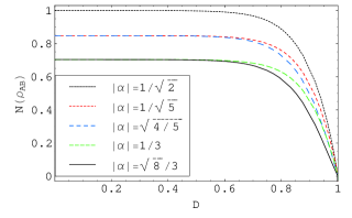
Figure 1: The logarithmic negativity as a function of the dilaton parameter $D$ with the fixed $\omega$ and $M$ for different $\alpha$.

The trajectories of the logarithmic negativity $N(\rho_{AB})$ versus $D$ for different $\alpha$ in Fig. 1 show how the dilaton parameter $D$ would change the properties of the entanglement. The logarithmic negativity $N(\rho_{AB})$ decreases as the dilaton parameter $D$ increases, which shows that the monotonous decrease of the entanglement with increasing $D$. It is interesting to note that except for the maximally entangled state, the same “initial entanglement” for $\alpha$ and $\sqrt{1-\alpha^{2}}$ will be degraded along two different trajectories, which just shows the inequivalence of the quantization for a scalar field in the dilaton black hole and Kruskal spacetimes. In the limit of $D\rightarrow M$, corresponding to the case of an extreme black hole, the logarithmic negativity is exactly zero for any $\alpha$, which indicates that the state has no longer distillable entanglement. This is due to the fact that the observer in the exterior of the GHS dilaton black hole detects a thermal Bose-Einstein distribution of particles given by Eqs. (18) as he traverses the Kruskal vacuum. This number of the particles $N_{\omega}^{2}\rightarrow\infty$ in the limit of $D\rightarrow M$, which means that the observer detected a maximally mixed state which contains no information.

We may also estimate the total correlations between Alice and Bob by use the mutual information RAM

$$I(\rho_{AB})=S(\rho_{A})+S(\rho_{B})-S(\rho_{AB}),$$ (24)

where $S(\rho)=-\text{Tr}(\rho\log_{2}\rho)$ is the entropy of the density matrix $\rho$. The mutual information quantifies how much information two correlated observers possess about one another’s state. The entropy of the joint state is

$$S(\rho_{AB})=-\sum_{n=0}^{\infty}e^{-8n\pi\omega(M-D)}[1-e^{-8\pi\omega(M-D)}]$$

$$\qquad\qquad~{}\times\left\{\alpha^{2}+(n+1)(1-\alpha^{2})[1-e^{-8\pi\omega(M-D)}]\right\}\log_{2}e^{-8n\pi\omega(M-D)}$$

$$\qquad\qquad~{}\times[1-e^{-8\pi\omega(M-D)}]\left\{\alpha^{2}+(n+1)(1-\alpha^{2})[1-e^{-8\pi\omega(M-D)}]\right\}.$$ (25)

We obtain Bob’s entropy in exterior region of the event horizon by tracing over Alice’s states for the density matrix $\rho_{AB}$

$$S(\rho_{B})=-\sum_{n=0}^{\infty}e^{-8n\pi\omega(M-D)}[1-e^{-8\pi\omega(M-D)}]\left\{\alpha^{2}+n(1-\alpha^{2})[e^{8\pi\omega(M-D)}-1]\right\}$$

$$\qquad\qquad\times\log_{2}e^{-8n\pi\omega(M-D)}[1-e^{-8\pi\omega(M-D)}]\left\{\alpha^{2}+n(1-\alpha^{2})[e^{8\pi\omega(M-D)}-1]\right\}.$$ (26)

Tracing over Bob’s states, we can also find Alice’s entropy can be expressed as

$$S(\rho_{A})=-[\alpha^{2}\log_{2}\alpha^{2}+(1-\alpha^{2})\log_{2}(1-\alpha^{2})].$$ (27)

Thus, we draw the behaviors of the mutual information $I(\rho_{AB})$ as a function of the dilaton parameter $D$ for different values of the state parameter $\alpha$ in Fig. 2.

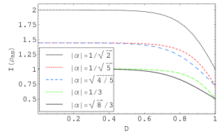
Figure 2: The mutual information as a function of the dilaton parameter $D$ with the fixed $\omega$ and $M$ for different $\alpha$.

Fig. 2 shows that as the dilaton parameter $D$ increases, the mutual information becomes smaller. Note that except for the maximally entangled state, the same “initially mutual information” for $\alpha$ and $\sqrt{1-\alpha^{2}}$ will be degraded along two different trajectories. In the limit of $D\rightarrow M$, the mutual information converges to the same nonvanishing minimum value again. Obviously if the “initially mutual information” is higher, it is degraded to a higher degree. Since the distillable entanglement in the limit $D\rightarrow M$ is exactly zero for any $\alpha$, we can say that the total correlations consist of classical correlations plus bound entanglement in this limit.

It is interesting to compare the results of the GHS black hole with those in the Schwarzschild one. For both the GHS and Schwarzschild cases, when describing the state (which involves tracing over the unaccessible modes), the observers find that some of the correlations are lost Pan Qiyuan due to the exterior region is causally disconnected from the interior region of the black hole. However, the entanglement is relevant to both the mass and dilaton parameters of the black hole in the GHS case, but it depends only on the mass of the black hole in the Schwarzschild case.

IV summary

We have analytically discussed the entanglement between two modes of a coupled massive scalar field as detected by Alice who stays stationary at an asymptotically flat region and Bob who locates near the event horizon in the background of a GHS dilaton black hole. It is shown that the entanglement does not depend on the mass of the particle and the coupling between the scalar field and the gravitational field, but it decreases with increasing dilaton parameter $D$. It is found that the same “initial entanglement” for the state parameter $\alpha$ and its “normalized partners” $\sqrt{1-\alpha^{2}}$ will be degraded along two different trajectories as the dilaton increases except for the maximally entangled state $\alpha=1/\sqrt{2}$, which just shows the inequivalence of the quantization for a scalar field in the dilaton black hole and Kruskal spacetimes. In the limit of $D\rightarrow M$, corresponding to the case of an extreme black hole, the state has no longer distillable entanglement for any $\alpha$. However, further analysis shows that the mutual information is degraded to a nonvanishing minimum value in this limit, which indicates that the total correlations consist of classical correlations plus bound entanglement.

References

• (1) D. Boschi, S. Branca, F. De Martini, L. Hardy, and S. Popescu, Phys. Rev. Lett. 80, 1121 (1998).
• (2) D. Bouwmeester, A. Ekert, and A. Zeilinger, The Physics of Quantum Information (Springer-Verlag, Berlin), 2000.
• (3) J. W. Pan, C. Simon, C. Brukner, and A. Zeilinger, Nature 410, 1067 (2001).
• (4) A. Peres and D. R. Terno, Rev. Mod. Phys. 76, 93 (2004).
• (5) P. M. Alsing and G. J. Milburn, Phys. Rev. Lett. 91, 180404 (2003).
• (6) Xian-Hui Ge and Sang Pyo Kim, Class. Quantum Grav. 25, 075011 (2008).
• (7) Yi Ling, Song He, Weigang Qiu, and Hongbao Zhang, J. Phys. A: Math. Theor. 40, 9025 (2007).
• (8) G. Adesso, I. Fuentes-Schuller, and M. Ericsson, Phys. Rev. A 76, 062112 (2007); G. Adesso and I. Fuentes-Schuller, arXiv:quant-ph/0702001.
• (9) I. Fuentes-Schuller and R. B. Mann, Phys. Rev. Lett. 95, 120404 (2005).
• (10) P. M. Alsing, I. Fuentes-Schuller, R. B. Mann, and T. E. Tessier, Phys. Rev. A 74, 032326 (2006).
• (11) Qiyuan Pan and Jiliang Jing, Phys. Rev. A 77, 024302 (2008).
• (12) W. G. Unruh, Phys. Rev. D 14, 870 (1976).
• (13) Qiyuan Pan and Jiliang Jing, Phys. Rev. D 78, 065015 (2008).
• (14) N. Arkani-Hamed, S. Dimopoulos, and G.Β R.Β Dvali, Phys. Lett. B 429, 263 (1998).
• (15) O. Dreyer, Phy. Rev. Lett. 90, 081301 (2003).
• (16) Songbai Chen and Jiliang Jing, Class. Quantum Grav. 22 533 (2005).
• (17) G. D. Birkhoff, Relativity and Modern Physics (Harvard University Press, Cambridge), 1927.
• (18) W. G. Unruh and R. M. Wald, Phys. Rev. D 25, 942 (1982).
• (19) D. Garfinkle, G. T. Horowitz, and A. Strominger, Phys. Rev. D 43, 3140 (1991); A. Gareia, D. Galtsov and O. Kechkin, Phys. Rev. Lett. 74 1276, (1995).
• (20) S. M. Barnett and P. M. Radmore, Methods in Theoretical Quantum Optics, 67-80 (Oxford University Press, New York), 1997.
• (21) D. Ahn, Phys. Rev. D 74, 084010 (2006).
• (22) A. Peres, Phys. Rev. Lett. 77, 1413 (1996).
• (23) G. Vidal and R. F. Werner, Phys. Rev. A 65, 032314 (2002).
• (24) M. B. Plenio, Phys. Rev. Lett. 95, 090503 (2005).
• (25) R. S. Ingarden, A. Kossakowski, and M. Ohya, Information Dynamics and Open Systems - Classical and Quantum Approach (Kluwer Academic Publishers, Dordrecht), 1997.