The effect of impurities on spin polarized Zeeman bound states in dilute magnetic semiconductor-superconductor hybrids

Abstract

We investigate the effect of single and multiple impurities on the Zeeman-localized, spin polarized bound states in dilute magnetic semiconductor hybrid system. Such bound states appear whenever a dilute magnetic semiconductor showing giant Zeeman effect is exposed to an external magnetic field showing nanoscale inhomogeneity. We consider the specific example of a superconductor-dilute magnetic semiconductor hybrid, calculate the energy spectrum and the wave functions of the bound states in the presence of a single impurity, and monitor the evolution of the bound state as a function of the impurity strength and impurity location with respect to the center of the Zeeman trapping potential. Our results have important experimental implications as they predict robust spin textures even for than than ideal samples. We find that for all realistic impurity strengths the Zeeman bound state survives the presence of the impurity. We also investigate the effect of a large number of impurities and perform ensemble averages with respect to the impurity locations. We find that the spin polarized Zeeman bound states are very robust, and they remain bound to the external field inhomogeneity throughout the experimentally relevant region of impurity concentration and scattering strength.

I Introduction

Due to its potential use in spintronics and quantum information applications, the controlled manipulation of individual spins has been a subject of great interest in recent years. In the search for appropriate materials for device fabrication, one possible route is the use of III-V or II-VI diluted magnetic semiconductors (DMS).

In II-VI DMSs, the exchange interaction between band charge carriers and the localized magnetic spins of the magnetic dopant (such as Mn) gives rise to a giant splitting between band states with different spin components. This giant Zeeman spin splitting has been extensively investigated and characterized. Furdyna1 Given the linear dependence of this splitting on the external applied magnetic field for fields lower than roughly 1T, it can be described in terms of a very large effective $g$-factor for the band carriers. For example, Dietl et al.Dietl1 reported an electron effective $g$-factor of about 500 at sub-Kelvin temperatures in a CdMnSe sample, which implies a value of about 2000 for the effective $g$-factor of a hole in this material. In previous works 03prl ; 05apl ; 05prb ; 05nature ; 06prb we proposed to take advantage of this large effective $g$-factor by combining it with a spatially inhomogeneous applied magnetic field, to create a spatially varying Zeeman potential that acts as a confining potential for only one spin orientation. In suitable conditions, this leads to a single charge carrier with a well defined spin being trapped in the region of large local magnetic field. This spin-polarized charged carrier can then be manipulated through external control on the applied inhomogeneous magnetic field.

The needed nanoscale inhomogeneous magnetic field can be generated in various ways. One possibility is to use nanoscale magnets placed above a DMS quantum well (QW).03prl ; 05apl ; 05prb ; peeters ; freire Depending on the shape and orientation of the nanomagnet, different nonuniform fields are generated, giving rise to various types of confined states.05prb

Another possibility is the use of Abrikosov vortices that appear in type-II superconductors (SCs). Above the lower critical field B${}_{c_{1}}$ vortices populate the superconductor, forming a vortex lattice. Nano-engineering can be used to insure that the vortices nucleate in well defined positions.nanosup The field of a single vortex is non-uniformly distributed around a core of radius $r\sim\xi$ ($\xi$ is the SC coherence length) and decays away from its maximum value at the vortex center over a length scale $\lambda$ ($\lambda$ is the penetration depth). If a SC layer that hosts such vortices is placed above a DMS layer (QW), the inhomogeneous magnetic field of the SC vortices creates an inhomogeneous magnetic field in the DMS layer. According to our previous calculations,05nature ; 06prb these fields are sufficiently large to result in the confinement of band carriers with a given spin orientation in the small region of the DMS QW that is located directly under a SC vortex core. Thus, spin textures are formed and can be manipulated by moving the source of the magnetic field, i.e. the SC vortex. In other words, the SC vortices act as spin and charge tweezers and can be used for a wide array of applications, from investigation of the Hofstadter butterfly and making spin shuttles05nature to generating anions of interest for topological quantum computing.marcel

In our previous work we assumed that the DMS QW is perfectly clean and with Mn impurities distributed in a perfectly homogeneous fashion (for instance by digital dopingdigitalDMS ), so that the Zeeman potential is a smooth function mirroring the applied magnetic field. For such systems we obtain typical binding energies of the spin-polarized charge carrier on the order of a few meV.05nature ; 06prb As we show in this paper, such perfect homogeneity is not necessary. This is a very important result from experimental detection and application point of view, since it opens up the possibility of investigating Zeeman localization effects in samples grown during standard molecular beam epitaxy (MBE) conditions. Since the effective $g$-factor is proportional to the local concentration of Mn, inhomogeneities in their distribution will result in a spatially-varying $g(\vec{r})$ which will modify the trapping potential. Even more detrimental are charged impurities which exist in any sample. Charge dopants are needed to introduce charge carriers in the II-VI DMS, because the Mn is isovalent with the valence-II element it replaces. The disorder due to these charged dopants can be minimized in the usual way used for two-dimensional electron systems, by doping at some distance away from the DMS QW and using gates to control the concentration of charge carriers in the DMS QW. However, small concentrations of undesired charged dopants in the DMS QW cannot be avoided.

In this article we investigate the role played by charged scattering centers on the confinement of spin polarized carriers in the DMS QW. We focus on repulsive centers, which are expected to be most detrimental to the binding of the spin-polarized carrier in the Zeeman trap, and then briefly discuss the other types of scattering centers mentioned above. We show that due to the difference between the length scale of the confining potential and the repulsive scattering potentials, the bound state energy is not significantly changed even in the presence of a large number of impurities. This result indicates that the binding of spin-polarized charge carriers in Zeeman traps created in a DMS QW is very robust against such defects, with immediate implications for spintronics applications based on this scenario.

It is important to also emphasize that our conclusions apply to a much wider range of systems than the one of interest to us, because these conclusions are based on quite simple physics, as we show below. We argue that in any system (such as quantum dots, quantum wells, etc.) where localization occurs on a lenghtscale much larger than that of typical scattering potentials, the effect of such scattering centers is very small even if their potential is very large.

This paper is organized as follows: In the next section we describe in more detail the system we study, our theoretical approach and the approximations we have made. In order to build intuition and to help interpret later calculations, in section III we analyze results for a simplified one dimensional (1D) model in the presence of a single impurity. This allows us both to gauge our computational scheme against exact solutions, and to gain some intuition about the effect of the scattering centers. In section IV we repeat the analysis for a single scattering center for the two-dimensional system of interest to us, and discuss the influence of the symmetries in our results. Finally, in section V we present results for a random distribution of impurities and various impurity concentrations. We conclude in section VI with a summary and discussion.

II Theoretical Model

The hybrid structure of interest to us is sketched in Fig. 1 (a), and consists of a SC layer in the vortex phase placed above a DMS QW. The two materials are separated by a thin insulating layer. The superconductor can be Pb or Ni, for example – both these metals can be grown on top of semiconductors using MBE techniques.bending The QW consists of a weakly p-doped DMS. An example of such a DMS QW is a p-doped (Cd,Mn)Te well, doped with N by a modulation doping technique that avoids inhomogeneity effects and increases the mobility of the carriers.dms2deg The carriers of interest to us are confined in the 2D DMS QW. The giant Zeeman effect in the DMS is described by a very large $g$-factor. This combines with the inhomogeneous magnetic field generated by each vortex to give rise to an effective potential that binds a spin polarized hole under each vortex, in a clean sample. As stated, we are now interested in the effect of repulsive scattering centers on these spin-polarized bounds states. A typical potential well in the presence of a single, and of several charged scatterers is illustrated in Figs. 1(b) and 1(c), respectively.

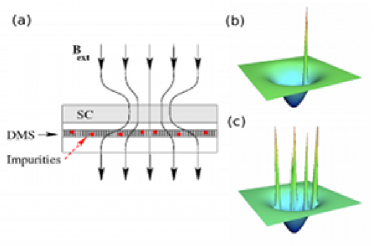
Figure 1: (color online) (a) Illustration of the magnetic field generated by a single vortex in a hybrid system made of a type II superconductor on top of a DMS quantum well which contains impurities. (b) Potential profile of the Zeeman trap plus a single repulsive impurity and (c) same, but for a random distribution of impurities (figures not to scale).

In a parabolic approximation, the Hamiltonian for a charge carrier in the 2D DMS quantum well which interacts with the magnetic field of the vortex and with scattering centers is

$$H=\frac{[\vec{p}-q\vec{A}(\vec{r})]^{2}}{2m}-\frac{1}{2}g_{\rm eff}\;\mu_{B}\vec{\sigma}\cdot\vec{B}(\vec{r})+\sum_{i}V_{i}(\vec{r}),$$ (1)

where $m$ and $q$ are the effective mass and charge of the carrier, $\vec{B}(\vec{r})$ is the magnetic field generated by a single vortex, $\vec{A}(\vec{r})$ is its vector potential and $V_{i}(\vec{r})$ are the repulsive potentials from the $i$ scattering centers. For simplicity, we assume that the motion of the carrier in the QW is two dimensional. In the calculations shown here, we use $m=0.5m_{e}$ and $g_{\rm eff}$=500, these being typical values for holes in II-VI semiconductors. Because of the large $g_{\rm eff}$, for a single vortex the effect of the $\vec{A}(x,y)$ term is negligible compared to that of the Zeeman interaction and we ignore it from now on.05nature

Experimental results show that the Zeeman splitting for holes in a DMS is anisotropic, depending on the direction of the magnetic field with respect to film plane.Kuhn1 Using a Luttinger Hamiltonian,Lut one can also show that in a 2D QW, the $g_{\rm eff}$ of heavy holes is highly anisotropic, with an in-plane component much smaller than that perpendicular to the film plane.05prb With these results in mind, we can further simplify our problem by considering only the effect of the $z$ component of the magnetic field, which is most strongly coupled to the charge carrier. This approximation allows us to decouple the Hamiltonian in the spin-up and spin-down sector, and consider them separately. We will only focus on the spin-component for which this Zeeman potential acts as a trap.

As discussed extensively in Ref. 05nature, , the size of the confining region defined by the inhomogeneous magnetic field depends on the superconductor’s parameters and the distance between the SC and DMS layers. It is typically several tens of nm in size. On the other hand, the impurity potential of the scattering centers is considerable only in a much smaller range of a few Å in the immediate vicinity of the impurity. It is the effect of this strong repulsive potential on the bound state that is of interest to us, since the long-range Coulomb repulsion is too weak to be relevant (although its effects can also be studied with our method, if so desired). Given the large difference between the characteristic length scales, we model the scattering potential as a delta function.

After all these approximations, the Schrödinger equation for the trapped spin component is:

$$\left[\frac{{p}^{2}}{2m}-g_{\rm eff}\mu_{B}\frac{\sigma}{2}B_{z}(\vec{r})+a\sum_{i}\delta(\vec{r}-\vec{R}_{i})\right]\psi_{\sigma}(\vec{r})=\varepsilon\psi_{\sigma}(\vec{r}),$$ (2)

where $a$ characterizes the strength of the impurity potential and $\vec{R}_{i}$ is the location of the $i^{th}$ impurity.

We solve for the eigenvalues in the usual way, by expanding the wavefunction in a complete basis set and finding the appropriate coefficients from a matrix equation. Our basis functions are B-spline polynomials on a non-uniform knot sequence adjusted optimally for each specific arrangement of charged impurities. This method has been widely used in atomic physics bsplines and is ideally suited for problems such as this. Details of the method and its advantages are discussed in the appendix A.

III One dimensional model

We first study a one dimensional model with a single delta function impurity inside a square potential well. This provides an intuitive understanding of the physics we want to explore, and also a numerical test of our B-spline scheme since it permits the comparison between the numerical results and the exact solution.

We consider a 1D square well potential

$$V_{0}(x)=\left\{\begin{array}[]{c l}-a_{0},&\mbox{if }-L/2\leq x\leq L/2\\ 0,&\mbox{otherwise}\end{array}\right.$$ (3)

where $L$ is the lateral size of the well. To it, we add a single impurity potential

$$V_{1}(x)=a\delta(x-x_{0})$$ (4)

where $x_{0}$ is the impurity position. In this case, the Schrödinger equation is given by

$$-\frac{\hbar^{2}}{2m}\frac{d^{2}}{dx^{2}}\psi(x)+V_{0}(x)+V_{1}(x)=\varepsilon\psi(x).$$ (5)

To understand the effects of the impurity on the bound states for different strengths of the impurity potential, we calculated the eigenvalues of this Hamiltonian. The energy of the lowest two bound eigenstates is shown in Fig. 2 vs. the strength of the impurity potential expressed as a dimensionless quantity $\alpha=a/(a_{0}L)$. The parameters are $L=100$nm and $a_{0}=3.5\hbar^{2}/(mL^{2})$, and the impurity is located in the center of the well, $x_{0}=0$. Fig. 2 reveals that the ground-state energy first increases with $\alpha$ and then saturates to the value of the first excited state. On the other hand, the energy of the first excited state is independent of $\alpha$. The reason for this behavior is straightforward to understand. Since the first excited state has a node at the location of the impurity, its energy and wavefunction is naturally unaffacted by its presence. On the other hand, the original ground state wavefunction has a maximum at the impurity location, so its energy increases with $\alpha$. However, for large enough $\alpha$ the ground-state wavefunction also develops a dip precisely at the location of the impurity and becomes insensitive to its strength. This is demonstrated by the insets to Fig.3, which show the ground-state wavefunction at $\alpha=0$ and $\alpha=100$. In essence, when $\alpha\gg 1$, the impurity potential splits the original well into two isolated wells which are degenerate, given the symmetry of the problem.

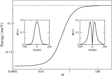
Figure 2: The ground state and first excited state energy versus $\alpha$, a dimensionless quantity related to strength of the impurity potential. The impurity is located at the center of the well $x=0$. The left inset shows the ground-state wavefunction for $\alpha=0$, and the right inset shows it for $\alpha=100$.

When the impurity is placed off-center, as in Fig. 3, the system loses this symmetry and the $\delta$ function separates the original well into two distinct wells of different sizes. Since the impurity is now placed in a location where both the original ground state and the first excited state wavefunction were finite, both energies now increase with $\alpha$ when $\alpha<1$. At higher values of $\alpha$ both the ground state and excited state energies saturate. As shown in the insets, the wavefunctions develop dips at the location of the impurity and become progressively more localized on one or the other smaller wells. The new ground state wavefunction becomes confined to the larger new well.

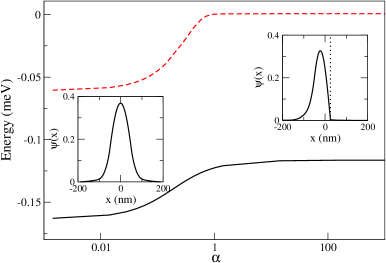
Figure 3: The ground state and first excited state energy versus the strength of the delta function impurity for $x_{0}=L/4$. $\alpha=a/a_{0}L$. The left inset shows the ground-state wavefunction for $\alpha=0$, and the right inset shows it for $\alpha=100$.

While these results are very easy to understand, they do provide key insight into the effects of the impurity on the bound states. First, it is clear that symmetry plays a very important role. While this influence is maximized by the one dimensional character of the model, we expect analogous features in the two-dimensional case.

More importantly, we already see that even if the impurity potential is large, its overall effect on the bound-state energy and wavefunction is limited. Because it is extended over a much larger area, the bound wavefunction simply avoids the impurity by developing a dip (or a zero) in its vicinity, at relatively low energetic cost. In 1D the impurity effectively “cuts” the wavefunction. This will not happen in $d=2$ or higher dimensions. However, as we demonstrate below, the limited effect on the binding energy is a general feature observed in higher dimensions.

The results shown so far also illustrate why B-splines are an ideal basis for such problems. If one tried to use a more traditional basis of orthonormal polynomials such as harmonic oscillator eigenstates, one would have to mix in very many basis states in order to be able to accurately describe smooth wave-function variations on a short length scale, near the impurity, as shown in the right inset of Fig. 2. Describing regions where the wavefunction essentially vanishes, as shown in the right inset of Fig. 3, would be even more difficult. On the other hand, use of B-splines allows one to just slightly increase the number of basis states by sampling the vicinity of the impurity on a smaller mesh. As a result, the calculation with one or more impurities is very comparable, in terms of numerical computational costs, with the one in the absence of impurities. A more detailed discussion of these issues is given in Appendix A.

IV Two dimensional Zeeman potential with a single impurity

We now can consider the two dimensional system in the presence of a single charged impurity. As we are not interested in the details of the Zeeman potential, we take the magnetic field generated by the vortex to have a Gaussian profile. This approximation is reasonable close to the vortex core, where the magnetic field decays exponentially on a length scale set by $\xi$.carneiro ; 05nature We therefore solve Eq. 2 where the magnetic field profile is taken to be:

$$B_{z}(\vec{r})=B_{0}\exp\left(-(\vec{r}-\vec{r}_{0})^{2}/\xi^{2}\right),$$ (6)

where $\vec{r}_{0}$ is the location of the vortex core, and $B_{0}=0.206$T and $\xi=50$ nm are the strength and the range of the magnetic field (these are typical values for a dirty Pb film in a type II regime). We solve the equation numerically for a system of finite size $200$nm $\times$ $200$nm, with periodic boundary condition and a grid of $51\times 51$ knots. This large lateral size is chosen so as to eliminate finite size effects in our bound state energies. For more details about the implementation of this numerical method and the periodic boundary conditions, see the appendix.

We follow a procedure similar to the one in the previous section and begin with a single impurity located at the center of the Gaussian and vary its potential strength. Again, we define a dimensionless quantity $\alpha=2a/(g_{\rm eff}\mu_{B}B_{0}\pi\xi^{2})$ related to the strength of the impurity potential. When the impurity is located at $\vec{r}_{0}$, as shown in Fig. 4 the ground state energy increases with the $\alpha$ and saturates at a finite value for $\alpha>0.01$. In the insets of Fig. 4, we can see that the ground-state wavefunction maintains its $s$-type symmetry as we increase $\alpha$ but develops a dip at its center. Similarly to the one dimensional case, the first excited state, which is two-fold degenerate, is not affected by the impurity potential, as can be seen in Fig. 5 (a) and (c). This is because its eigenfunctions have $p$-type symmetry, with a node at the origin where the impurity is located. These results mirror those of the 1D case but are less dramatic: the energy separation $\Delta$E between the two lowest eigenstates changes by less than 30% for arbitrarily strong repulsive impurity potentials even when the charged impurity is placed where it should do the most damage.

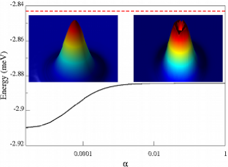
Figure 4: (color online) The two lowest state energies versus the impurity strength. The left(right) inset is the ground-state wavefunction for $\alpha=0$ ( $\alpha=1$).

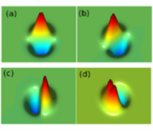
Figure 5: (color online) Wave-functions of the two excited states with $p$-type symmetry when the impurity is located at the center of the vortex, in (a) and (c); and for an off-center impurity, in (b) and (b).

Next, we investigate the dependence of the bound energies and wave-functions on the location of the impurity, for a fixed strength $\alpha$. The results are shown in Fig.6. The ground state energy decreases monotonically as the impurity moves away from the vortex center because it costs less energy to create a dip at its location (the ground-state wavefunction is shown in the inset). Once the impurity is farther away than the characteristic length scale of the bound state, the ground-state energy saturates to its unperturbed value. Due to the symmetry of the problem, the degeneracy of the first excites state is lifted. The state which has its nodal line where the impurity is located is unaffacted by it. The other eigenstate has a finite wavefunction at the impurity location, and its energy is increased. However, if the impurity is placed far enough, its effect vanishes and the two excited eigenstates become degenerate again. The excited wavefunctions are shown in Figs.5(b) and (d).

Finally, we analyze how the energies of the lowest eigenstates change when the impurity is off-center at a fixed distance $r_{i}=5$ nm and we vary the impurity strength. The results are shown in Fig. 7. As expected, the ground-state energy increases but very little, since for large $\alpha$ a dip appears at the location of the impurity and its effect saturates, irrespective of its strength. The excited state with a nodal line at the impurity location continues to be unaffected by it, while the other excited state behaves similarly to the ground-state: its energy increases with $\alpha$, but only by a finite amount until its wavefunction acquires a zero where the impurity is.

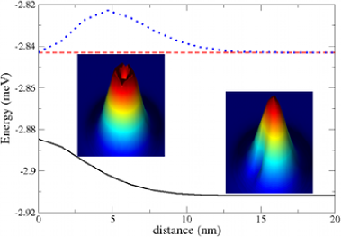
Figure 6: (color online) The lowest eigenenergies versus the distance of the impurity from the center of the vortex. The solid line is the ground state energy, the dashed line is the energy of the excited state whose wavefunction is shown in Fig. 5 while the other excited state’s wavefunction is shown in Fig. 5 (d). The left (right) inset is the ground-state wavefunction for $r_{i}=0$ ($r_{i}=5$ nm).

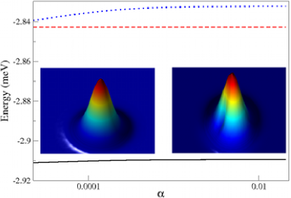
Figure 7: The ground, first and second excited state energy versus the impurity strength. The left inset is the wavefunction for $\alpha=0$, and the right inset is the wavefunction for $\alpha=0.01$.

These results clearly demonstrate that a single impurity is unable to unbind the Zeeman trapped charge carrier, irrespective of how large its repulsive potential is. All it can do is to simply “poke a hole” in the wavefunction, and this costs a relatively small energy. Even if the impurity is placed at the center of the Zeeman potential well, the energetic cost is little. This suggests that one could have many impurities in the vortex area without affecting the bound state significantly. Our expectations are indeed verified in the next section.

V Random distribution of impurities

We now address a more realistic situation of a random distribution of multiple impurities inside the QW. In this case, as detailed in the appendix, the use of B-splines is particularly useful to minimize computational costs.

For a large number of impurities, the energy and wave function will depend on the distribution of impurities. We follow the standard procedure and average our results over various impurity configurations. We performed averages over 1000 configurations at different impurity concentrations. The digitally doped Cd_1-xMn_xTe has a Zinc-Blende structure with a lattice constant of about $6.5\AA$. There are 4 Cd in an unit cell, and we take $x\sim 1.6$. Assuming a single layer of Cd_1-xMn_xTe gives a Mn areal concentration of $0.15$ nm^-2. As already discussed, the number of charged dopants can be minimized by the use of co-doping techniques. While is impossible to eliminate all these scattering centers, we expect that their concentration is much smaller than the Mn concentration.

Fig. 8 shows the central result of this work: the average ground-state energy of the bound state increases linearly with the concentration of impurities, however the slope is very small. Thus, for any reasonable concentration of impurities we see that their effect on the bound state energy is very minimal. This is fully expected, given the analysis presented in the previous sections. Moreover, those results also imply that increasing the relative strength $\alpha$ of the scattering potentials will not change this conclusion, since the effect of each scatterer saturates at large $\alpha$.

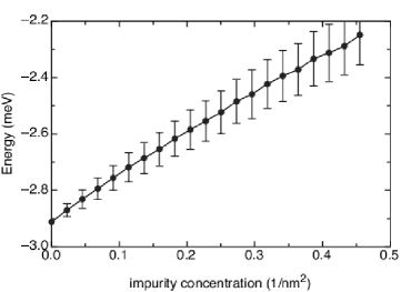
Figure 8: The ground state energy versus the impurity concentration. The energy was averaged over 1000 different impurity distributions and we chose $\alpha=0.005$.

Finally, we comment briefly on the effects of other types of scatterers mentioned in the introduction. Clearly, attractive impurities cannot unbind the spin-polarized charge carrier – to the contrary, they will bind it more strongly. Weak scatterers will have small, perturbational effects on the bound state. If the attractive potential is extremely strong, a charge carrier becomes bound to the impurity itself and will screen its potential, making the scatterer “invisible” to the spin-polarized charge carrier trapped by the Zeeman potential. We conclude that such scatterers cannot damage the bound state.

The other potential source of scattering is due to “noise” in the values of $g_{\rm eff}$ reflecting the variations in the local density of Mn. One expects the typical scale for such variations (especially in digitally doped layers) to be very short compared to the tens of nm length scale of the bound wavefunction. If we model it in terms of a sum of short-range (delta function) noise, the conclusions will be as above, especially since the typical variation must be a small fraction of the average $g_{\rm eff}$, i.e. we expect this to be in a weak-scatterer regime.

VI Conclusions

In this article we studied the effect of single and multiple impurities on the spin-polarized state bound by a trapping potential generated by an inhomogeneous magnetic field in a diluted magnetic semiconductor QW. We demonstrated that this effect is very limited, because of the large difference in length scales between the size of the wavefunction and the typical size of a strong scattering potential. For very large scattering potentials, each impurity pokes a hole in the bound wavefunction, at a very small energetic cost. As a result, even for large concentrations of very strong scatterers, the overall effect on the bound state is very limited.

This result has obvious positive implications for any applications based on such trapped states, since they show that it is not necessary to worry about the effects of impurities or to use expensive methods to eliminate them. Samples grown in reasonably clean conditions should suffice for devices based on these spin-polarized, Zeeman-trapped states.

Appendix A B-splines

B-splines have long been employed successfully in atomic and molecular physics,bsplines but are not as freqently used in condensed matter physics.splinessol The aim of this appendix is to give a brief intuitive picture of the B-splines and their usefulness for solving Schrödinger equations with complicated potentials. Many more details on B-splines and their uses are available in the literature.bsplines

B-splines are piecewise polynomials and therefore are well suited for interpolation, having been extensively used in fitting tools, including many commercial software applications.soft In the context of interest to us, they are used as a basis in which to expand the eigenfunctions. Of course, there are many possible finite basis sets and finite elements methods that can be used to solve a Schrödinger equations. The main advantage of using B-splines is the flexibility to choose the grid points on which the B-splines are defined. If we need to describe slowly-varying functions, a large mesh suffices, resulting in a small basis set. In regions where there are fast variations, one can use a finer local mesh, optimized to give the desired accuracy for the minimum increase in the number of basis functions. Furthermore, because the B-splines are piecewise polynomials, matrix elements can be efficiently evaluated to machine accuracy with Gaussian integration. Finally, the banded nature and sparsity of the resulting matrices allows for the use of very large basis sets, if need be.

Suppose that we need to approximate a 1D function in a given interval $x\in[a,b]$. We first define a knot-sequence of points in this interval $\{x_{i}|a=x_{0}\leq x_{1}\leq x_{2}\leq...\leq x_{N}=b\}$. The location of the points as well as their number will be chosen so as to optimize the process. For instance, the knot-sequence can consist of regions of equally spaced knots combined with regions where the knots are space in an exponential fashion, or any other suitable scheme. On this knot-sequence, we define the normalized B-splines of rank $k$ by the following recursion relation:

$$B_{i,1}(x)=\left\{\begin{array}[]{c l}1,&\mbox{if }x_{i}\leq x<x_{i+1}\\ 0,&\mbox{otherwise}\end{array}\right.$$ (7)

and

$$B_{i,k}(x)=\frac{x-x_{i}}{x_{i+k-1}-x_{i}}B_{i,k-1}(x)+\frac{x_{i+k}-x}{x_{i+k}-x_{i+1}}B_{i+1,k-1}(x)$$ (8)

where $i$ is the index of a knot point and $k$ is the order of the spline. Thus, the $B_{i,k}(x)$ is a polynomial of order $k-1$ defined piece-wise in the interval $[x_{i},x_{i+k}]$, and vanishing outside it. Moreover, all derivatives up to the order of $k-2$ are also continuous. Since we use these functions to expand eigenstates, which are continuous and have first and second continuous derivatives, it follows we should use a cubic ($k=4$) or higher order B-splines. Here we use cubic splines, as they are the simplest splines with the desired properties. From now on, we simplify our notation and use $B_{i}(x)$ to mean the cubic B-spline. The function of interest is then expanded in terms of these splines:

$$f(x)=\sum_{i}\alpha_{i}B_{i}(x)$$ (9)

where $\alpha$ are the $N+3$ coefficients of our expansion (for the $N+1$-point knot sequence).

To solve an eigenvalue problem, we expand the wavefunction in terms of B-splines and reduce the problem to a general matrix system:

$$\mathbf{H}-\varepsilon\mathbf{S}\mathbf{v}=0,$$ (10)

where $\mathbf{H}$ is the Hamiltonian matrix, $\mathbf{S}$ is the overlap matrix and $\mathbf{v}$ is the eigenvector containing the unknown coefficients for the various B-splines. For a 1D Schrödinger equation with a potential $V(x)$, the matrix elements of $\mathbf{H}$ and $\mathbf{S}$ are equal to:

$$H_{i,j} = \frac{1}{2m}\int{dB_{i}(x)\over dx}\frac{dB_{j}(x)}{dx}dx+\int B_{i}(x)V(x)B_{j}(x)dx$$

$$S_{i,j} = \int B_{i}(x)B_{j}(x)dx$$ (11)

where we used an integration by parts in the kinetic energy. The integrals for the kinetic energy and the overlap can be evaluated analytically, while those of the potential may need numerical integration, if $V(x)$ is a complicated function. However, given the finite support of each B-spline, such matrix elements are non-vanishing only if $|i-j|<k$, so the number of needed integrals scales like the number of basis functions, not like its square, as is the case for most other basis.

The choice of the knot sequence plays an important role in these solutions. A good choice of knots distribution can assure a fast convergence to the true eigenenergy with a small basis set. To illustrate this, we consider a gaussian potential and we calculate the ground-state eigenvalue and eigenfunction using two different knot sequences. As illustrated in Fig 9, one is a uniform distribution of knots, while the other has an exponential distribution of knots from the center of the potential. In the inset of Fig 9, we compare the convergence of the energy as a function of the number of knots. It is clear that the non-uniform distribution is much more efficient in this case, giving a very accurate wavefunction and eigenenergy for a sequence with very few knots, i.e. a very small basis set.

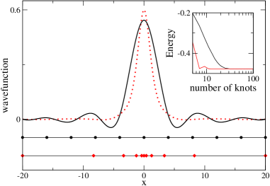
Figure 9: The dots on the two lower lines illustrate the uniform (squares) and non-uniform (diamonds) knot sequences. The curves show the estimated ground-state wavefunction for these $N=11$ knot sequences, full line for the uniform and the dotted line for the non-uniform one. The inset shows the convergence of the energy to the true value as a function of the number $N$ of knots used.

In the atomic physics, rigid boundaries are normally used when working with B-splines. Since in solid state physics we sometimes want to investigate bulk and transport properties, we opted to generalize the B-spline method to periodic boundary conditions. The periodic conditions for B-spline are constructed in the following way (for cubic splines, although the generalization to higher orders is straightforward). Suppose we want B-spines on the support of the knot sequence $\{x_{i}|a=x_{0}\leq x_{1}\leq x_{2}\leq...\leq x_{N}=b\}$,

i) Expand the knot sequence $\{x_{i}\}$ to $\{x^{\prime}_{i}\}$ by adding the knots:

$$x^{\prime}_{-2} = x_{N-2}-(b-a)$$ (12)

$$x^{\prime}_{-1} = x_{N-1}-(b-a).$$ (13)

Note that since $x^{\prime}_{-1}$ and $x^{\prime}_{-2}<a$, they are outside the interval of interest.

ii) Construct the B-splines $\{B^{0}_{i}\}$ with the usual procedure on the new support $\{x^{\prime}_{i}\}$. Note that the first two B-splines, which we call $B^{0}_{-3},B^{0}_{-2}$ have finite support outside our desired interval.

iii) Now construct the B-splines $\{B_{i}\}$ by moving the pieces of $B^{0}_{i}$ defined outside the interval of interest, to inside $[a,b]$ by a translation of period $(b-a)$.

Following the above procedure, all $\{B_{i}(x)\}$ are periodic functions with period $(b-a)$. Hence the functions in the Hilbert space expanded by $\{B_{i}(x)\}$ with coefficients $c_{i}^{\prime}s$:

$$f(x)=\sum_{i}c_{i}B_{i}(x)$$ (14)

are all periodic, thus ensuring the periodic boundary condition. Of course, for our problem of interest we choose $b-a$ to be large enough that the localized wavefunction is all fully contained inside it. In other words, increasing $b-a$ has no effect on the eigenenergies we calculate.

The generalization to two-dimensional or higher-dimensional systems is straightforward. The wavefunction needs to be expanded in products of B-splines

$$\psi(x,y)=\sum_{i}\alpha_{i,j}B_{i}(x)B_{j}(y)$$ (15)

and all the procedures above can be repeated. For our problem, we simply choose a high-density of knots in the immediate neighborhood of each impurity, where the wavefunctions change rapidly, and a wide, exponential mesh everywhere else, where the function changes slowly. The mesh near each scatterer has been optimized till convergence is reached.

References

- (1) H. Ohno, Appl. Phys. Lett. 69, 262 (1996).
- (2) J. K. Furdyna, J. Appl. Phys. 64, R29 (1988).
- (3) T. Dietl, M. Sawicki, M. Dahl, D. Heiman, E. D. Isaacs, M. J. Graf, S. I. Gubarev, and D. L. Alov, Phys. Rev. B 43, 3154 (1991).
- (4) M. Berciu, and B. Janko, Phys. Rev. Lett. 90, 246804 (2003).
- (5) R. Fiederling, M. Keim, G. Reuscher, W. Ossau G. Schmidt, A. Waag, and L. W. Molenkamp, Nature (London) 402, 787(1999).
- (6) P. Redlinski, T. G. Rappoport, A. Libal, J. K. Furdyna, B. Janko, and T. Wojtowicz, Appl. Phys. Lett. 86, 113103(2005).
- (7) P. Redlinski, T. Wojtowicz, T. G. Rappoport, A. Libal, J. K. Furdyna, and B. Janko, Phys. Rev. B 72, 085209(2005).
- (8) M. Berciu, T. G. Rappoport, and B. Janko, Nature (London) 435, 71 (2005).
- (9) T. G. Rappoport, M. Berciu, and B. Jankó, Phys. Rev. B 74, 094502 (2006).
- (10) F. M. Peeters, and A. Matulis, Phys. Rev. B 48, 15166 (1993).
- (11) J. A. K. Freire, A. Matulis, F. M. Peeters, V. N. Freire, and G. A. Farias, Phys. Rev. B 61, 2895 (2000).
- (12) J. Jaroszynski et al., Phys. Rev. Lett 89, 266802 (2002); B. Jussereand et al., Phys. Rev. Lett. 91, 086802 (2003); R. Knobel, N. Samarth, J. G. E. Harris and D. D. Awschalom, Phys. Rev. B 65, 235327 (2002); M. Goryca et al., Phys. Rev. Lett. 102, 046408 (2009).
- (13) J. Van de Vondel, C. C. de Souza Silva, B. Y. Zhu, M. Morelle, and V. V. Moshchalkov, Phys. Rev. Lett. 94, 057003 (2005)
- (14) C. Weeks, G. Rosenberg, B. Seradjeh and M. Franz, Nature Physics 3, 796 (2007).
- (15) R. W. Kawakami, E. Johnston-Halperin, L. F. Chen, M. Hanson, N. Guebels, J. S. Speck, A. C. Gossard, and D. D. Awschalom Appl. Phys. Lett. 77, 2379 (2000); T. C. Kreutz, G. Zanelatto, E. G. Gwinn, and A. C. Gossard, Phys. Lett. 81, 4766 (2002).
- (16) S. J. Bending, K. von Klitzing, and K. Ploog, Phys. Rev. Lett. 65, 1060 (1990); A. K. Geim, S. J. Bending, and I. V. Grigorieva, Phys. Rev. Lett. 69, 2252 (1992).
- (17) B. Kuhn-Heinrich, W. Ossau, H. Heinke, F. Fischer, T. Liz, A. Waag, and G. Landwehr, Appl. Phys. Lett. 63, 2932 (1993).
- (18) J. M. Luttinger and W. Kohn, Phys. Rev. 97, 869 (1955).
- (19) H. Bachau, E. Cormier, P. Decleva , J. E. Hansen and F Martin, Rep. Prog. Phys. 64 (2001); J. Sapirstein and W. R. Johnson J. Phys. B: At. Mol. Opt. Phys. 29 (1996).
- (20) G. Carneiro and E. H. Brandt, Phys. Rev. B 61, 6370 (2000).
- (21) See for example, Microcal Origin and Matlab.
- (22) J. Sanchez-Dehesa, J. A. Porto, F. Agullo-Rueda and F. Meseguer, J. Appi. Phys. 73 (1993).