Bi-directional mapping between polarization and spatially encoded photonic qutrits

Abstract

Qutrits, the triple level quantum systems in various forms, have been proposed for quantum information processing recently. By the methods presented in this paper a bi-photonic qutrit, which is encoded with the polarizations of two photons in the same spatial-temporal mode, can be mapped to a single photon qutrit in spatial modes. It will make arbitrary unitary operation on such bi-photonic qutrit possible if we can also realize the inverse map to polarization space. Among the two schemes proposed in this paper, the one based only on linear optics realizes an arbitrary $U(3)$ operation with a very small success probability. However, if added with weak nonlinearity, the success probability can be greatly improved. These schemes are feasible with the current experimental technology.

I Introduction

Quantum communications and quantum computation apply quantum states to store and transmit information. The capacity of a state for the purpose is dependent on its dimension, so the higher dimension of a state means the higher capacity to carry information. In addition, the use of higher dimensional quantum states, e.g., qudits and entangled qudits, enjoys many advantages such as enhanced security in quantum cryptography Langford , more efficient quantum logic gate Ralph and others. Qudits and entangled qudits therefore attract many researches recently. The proposals for generating qudits and entangled qudits include orbital angular momentum entangled qutrits Mair , pixel entangled qudits Neves , energy-time entangled and time-bin entangled qudits Thew , and bi-photonic qutrits encoded with polarization degree of freedom Howell ; Mikami ; Lanyon . In this paper we will focus on bi-photonic qutrits which are represented with the polarizations of two photons in the same spatial-temporal mode note —$\left|0\right\rangle_{3}\equiv\left|HH\right\rangle$, $\left|1\right\rangle_{3}\equiv\left|HV\right\rangle$, and $\left|2\right\rangle_{3}\equiv\left|VV\right\rangle$, where $H$ and $V$ denotes the horizontal and vertical polarization, respectively. The generation of such qutrits including the entangled ones has been demonstrated Howell ; Lanyon . In an recent work by Lanyon, et al. Lanyon , with an ancilla qubit and a Fock state filter associated with some wave plates, a bi-photonic state as the linear combination of $\{\left|0\right\rangle_{3},\left|1\right\rangle_{3},\left|2\right\rangle_{3}\}$ is generated from the logic state $\left|0\right\rangle_{3}$. To manipulate a bi-photonic qutrit in this form, one should know how to implement a unitary operation on such qutrits. However, due to the indistinguishableness of two photons in the same spatial-temporal mode, it is very difficult to realize a simple unitary operation on such bi-photonic qutrit Bogdanov . Here we present two schemes realizing the transformation from a bi-photonic qutrit to any other bi-photonic qutrit, i. e., arbitrary unitary operations $U(3)$ on bi-photonic qutrits. The schemes work with transforming the input bi-photonic qutrits to the corresponding single photon qutrits in spatial modes, and then mapping the single photon qutrits back to the original polarization modes of two photons.

The rest of the paper is organized as follows. In Sec. II, we present a purely linear optical scheme of the transformation and inverse transformation from a bi-photonic qutrit in the same spatial-temporal mode to the corresponding single photon qutrit. In Sec. III, we improve on the linear optical scheme with weak cross-Kerr nonlinearity, making the realization of bi-directional mapping much more efficient. Sec. IV concludes the work with a brief discussion.

II
Bi-directional mapping with linear optical elements

Any unitary operation on a single photon qudits in spatial modes can be performed by a linear optical multi-port interferometer (LOMI) Reck . It is therefore possible to manipulate bi-photonic qutrits following such strategy—first transforms a bi-photonic qutrit to a single-photon qutrit, and then performs the desired operations on this single photon qutrit, and finally transforms the single photon qutrit back to a bi-photonic qutrit. In what follows, we present the details of the procedure, which is realized only with linear optical elements.

II.1
Transforming bi-photon qutrit to single-photon qutrit

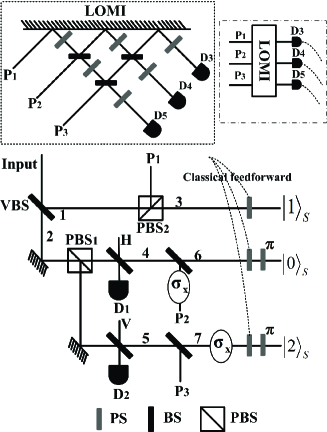
Figure 1: Schematic setup for the transformation from a bi-photonic qutrit to the corresponding single-photon qutrit. At first, the input qutrit is transmitted through a VBS, and then the two output modes are transmitted through a PBS, respectively. Two single photons are used as the ancillas, which will interfere with the output modes of PBS₁. The part in dashed line is used to erase the path information of the modes $P_{1},P_{2},P_{3}$, which are all in the state $\left|V\right\rangle$. The detection results are used as control signals of the conditional phase shift summarized in Tab. I through the classical feed-forward. By the proper post-selection, the bi-photonic qutrit can be transformed to the corresponding single-photon qutrit as in Eq. (2). For details, see the text.

Suppose a bi-photonic qutrit is initially prepared as

$$\left|\psi\right\rangle_{in}=\alpha\left|0\right\rangle_{3}+\beta\left|1\right\rangle_{3}+\gamma\left|2\right\rangle_{3},$$ (1)

where $\left|\alpha\right|^{2}+\left|\beta\right|^{2}+\left|\gamma\right|^{2}=1$. The operations shown in Fig. 1 implements the map

$$\left|\psi\right\rangle_{in}\rightarrow\alpha\left|0\right\rangle_{S}+\beta\left|1\right\rangle_{S}+\gamma\left|2\right\rangle_{S}=\left|\psi\right\rangle_{S},$$ (2)

where $\left|\psi\right\rangle_{S}$ is a single-photon qutrit encoded with the spatial modes $|i\rangle_{S}$ ($i=0,1,2$) of the single photon. Here we first apply a variable beam splitter (VBS) to the input bi-photonic qutrit, realizing the following transformation

$$\left(\frac{\alpha}{\sqrt{2}}a_{H}^{\dagger 2}+\beta a_{H}^{\dagger}a_{V}^{\dagger}+\frac{\gamma}{\sqrt{2}}a_{V}^{\dagger 2}\right)\left|vac\right\rangle$$

$$\rightarrow\left[\frac{\alpha}{\sqrt{2}}\left(ra_{H1}^{\dagger}+ta_{H2}^{\dagger}\right)^{2}+\beta\left(ra_{H1}^{\dagger}+ta_{H2}^{\dagger}\right)\right.$$

$$\times\left.\left(ra_{V1}^{\dagger}+ta_{V2}^{\dagger}\right)+\frac{\gamma}{\sqrt{2}}\left(ra_{V1}^{\dagger}+ta_{V2}^{\dagger}\right)^{2}\right]\left|vac\right\rangle,$$ (3)

where $1$, $2$ denote the different paths, and $t$ $(r)$ is the transmissivity (reflectivity) of the VBS.

Next, in order to project out the proper components, we introduce two single photons $\left|H\right\rangle$ and $\left|V\right\rangle$ as the ancilla, and make them interfere with the output modes of the polarizing beam splitters (PBS₁) on two 50:50 beam splitters (BS), respectively. Due to the Hong-Ou-Mandal interference effect Hong , two indistinguishable photon will be bunching to the same output mode of BS, and then we can use the proper post-selection to get the desired components. To see the details, we show the evolution of each input mode of two photons as follows:

$$a_{H1}^{\dagger} \rightarrow a_{H3}^{\dagger},a_{H2}^{\dagger}\rightarrow\frac{1}{\sqrt{2}}\left(a_{H4}^{\dagger}+a_{HD_{1}}^{\dagger}\right),$$

$$a_{V1}^{\dagger} \rightarrow a_{VP_{1}}^{\dagger},a_{V2}^{\dagger}\rightarrow\frac{1}{\sqrt{2}}\left(a_{V5}^{\dagger}+a_{VD_{2}}^{\dagger}\right),$$ (4)

where the subscripts $D_{1},D_{2}$ denote the modes going to photon number non-resolving detectors. Meanwhile, for the ancilla photons, the evolutions are

$$a_{H}^{\dagger} \rightarrow\frac{1}{\sqrt{2}}\left(a_{H4}^{\dagger}-a_{HD_{1}}^{\dagger}\right),\$$

$$a_{V}^{\dagger} \rightarrow\frac{1}{\sqrt{2}}\left(a_{V5}^{\dagger}-a_{VD_{2}}^{\dagger}\right).$$ (5)

The 50:50 BS placed on path 4 (5) is to split the mode 4 (5) into two output modes 6, P₂ (7, P₃), making the transformations,

$$a_{H4}^{\dagger} \rightarrow\frac{1}{\sqrt{2}}\left(a_{H6}^{\dagger}+a_{HP_{2}}^{\dagger}\right)\rightarrow\frac{1}{\sqrt{2}}\left(a_{H6}^{\dagger}+a_{VP_{2}}^{\dagger}\right),$$

$$a_{V5}^{\dagger} \rightarrow\frac{1}{\sqrt{2}}\left(a_{V7}^{\dagger}+a_{VP_{3}}^{\dagger}\right)\rightarrow\frac{1}{\sqrt{2}}\left(a_{H7}^{\dagger}+a_{VP_{3}}^{\dagger}\right).$$ (6)

After that, one obtains the following state:

$$\left(-\frac{\alpha}{4\sqrt{2}}t^{2}a_{H6}^{\dagger}a_{VP_{2}}^{\dagger}+\frac{\beta}{2}r^{2}a_{H3}^{\dagger}a_{VP_{1}}^{\dagger}-\frac{\gamma}{4\sqrt{2}}t^{2}a_{V7}^{\dagger}a_{VP_{3}}^{\dagger}\right)$$

$$\times a_{HD_{1}}^{\dagger}a_{VD_{2}}^{\dagger}\left|vac\right\rangle+rest.$$ (7)

where $rest.$ denotes the components of two photons appearing in the same spatial mode. If we discard the modes $P_{1},P_{2},P_{3}$ without changing anything else, i.e., erase the path information of $P_{1},P_{2},P_{3}$, the first three terms in Eq. (7) will be just the desired single photon qutrit, which carries the same coefficients of the input bi-photon qutrit. Since there is only one photon in the modes $P_{1},P_{2},P_{3}$, we will use a quantum Fourier transform (QFT) ($j,k^{\prime}$ denote the spatial modes) Nielsen ,

$$a_{Vj}^{\dagger}\left|vac\right\rangle=\frac{1}{\sqrt{3}}\overset{2}{\underset{k^{\prime}=0}{{\sum}}}e^{2\pi ijk/3}a_{Vk^{\prime}}^{\dagger}\left|vac\right\rangle,$$ (8)

to do it. The QFT is an unitary operation for a single photon in three spatial modes, so we can use an LOMI shown in the dashed line of Fig. 1 to implement it. Just like the setups in the dash-dotted line, three photon number non-resolving detectors are used and the detection results are to control the conditional phase shift (PS) through classical feedforward. The relations between the detection results and the corresponding PS operations are summarized in Tab. 1.

$\begin{array}[c]{|c|c|c|c|}\hline\cr&D_{3}&D_{4}&D_{5}\\ \hline\cr 3&0&0&0\\ \hline\cr 6&0&\frac{2\pi}{3}&\frac{4\pi}{3}\\ \hline\cr 7&0&\frac{4\pi}{3}&\frac{8\pi}{3}\\ \hline\cr\end{array}$

Table 1: The relations between the detections and the corresponding phase shifters on path 3, 6, 7.

After that, with the coincident measurements of the detectors $D_{1}$, $D_{2}$, and one of the detectors $D_{3},D_{4},D_{5}$, the state

$$\left(\frac{\alpha}{4\sqrt{2}}t^{2}a_{H6}^{\dagger}+\frac{\beta}{2}r^{2}a_{H3}^{\dagger}+\frac{\gamma}{4\sqrt{2}}t^{2}a_{V7}^{\dagger}\right)\left|vac\right\rangle,$$ (9)

will be projected out by the post-selection. We can rewrite it as

$$\frac{\alpha}{4\sqrt{2}}t^{2}\left|H\right\rangle_{6}+\frac{\beta}{2}r^{2}\left|H\right\rangle_{3}+\frac{\gamma}{4\sqrt{2}}t^{2}\left|V\right\rangle_{7}.$$ (10)

It is straightforward that the state will be $\left|\psi\right\rangle_{S}$, given that $t^{2}=2\sqrt{2}r^{2}$ or $t^{2}=\frac{2\sqrt{2}}{1+2\sqrt{2}}$. The corresponding success probability of the process is $\left(\frac{t^{2}}{4\sqrt{2}}\right)^{2}=1.71\times 10^{-2}.$

II.2 Transformation back to bi-photonic qutrit

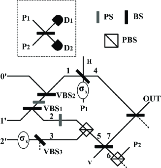
Figure 2: Schematic setup for the inverse transformation from a single-photon qutrit back to a bi-photon qutrit. Two variable beam splitters (VBS) are applied, and two extra single photon work as the ancilla. The single-photon qutrit can be transformed back to a bi-photonic qutrit by post-selection. For details, see the text.

After the desired operations performed on the single photon qutirt, we should transform the single-photon qutrit $\left|\psi^{{}^{\prime}}\right\rangle_{S}=\alpha^{{}^{\prime}}\left|0^{{}^{\prime}}\right\rangle_{S}+\beta^{{}^{\prime}}\left|1^{{}^{\prime}}\right\rangle_{S}+\gamma^{{}^{\prime}}\left|2^{\prime}\right\rangle_{S}$ back to a bi-photonic qutrit. The inverse transformation is shown in Fig. 2. Three VBSs (VBS₁, VBS₂, VBS₃) with the transmissivities (reflectivities) $t_{1}$, $t_{2}$, $t_{3}$ ($r_{1}$, $r_{2}$, $r_{3}$), two PSs and $\sigma_{x}$ operation are applied to perform the transformation

$$\left(\alpha^{{}^{\prime}}a_{H0^{{}^{\prime}}}^{\dagger}+\beta^{{}^{\prime}}a_{H1^{{}^{\prime}}}^{\dagger}+\gamma^{{}^{\prime}}a_{H2^{{}^{\prime}}}^{\dagger}\right)\left|vac\right\rangle$$

$$\rightarrow\left[\left(\alpha^{{}^{\prime}}r_{2}-\beta^{{}^{\prime}}t_{1}t_{2}\right)a_{H1}^{\dagger}+\beta^{{}^{\prime}}r_{1}a_{H2}^{\dagger}+\gamma^{{}^{\prime}}t_{3}a_{V3}^{\dagger}\right]\left|vac\right\rangle.$$ (11)

In order to select out the desired components, we introduce a single photon $\left|H\right\rangle$ as an ancilla, which will interfere with the mode 1 through a 50:50 BS, and meanwhile combine the modes 2 and 3 by a PBS into the mode 5, which will then interfere with another ancilla single photon $\left|V\right\rangle$ through a 50:50 BS. The total state will be then transformed to

$$\left\{\frac{1}{2\sqrt{2}}\left(\alpha^{{}^{\prime}}r_{2}-\beta^{{}^{\prime}}t_{1}t_{2}\right)\left(a_{H4}^{\dagger 2}-a_{HP_{1}}^{\dagger 2}\right)\left(a_{V7}^{\dagger}-a_{V6}^{\dagger}\right)\right.$$

$$+\frac{1}{2\sqrt{2}}\beta^{{}^{\prime}}r_{1}\left(a_{H4}^{\dagger}-a_{HP_{1}}^{\dagger}\right)\left(a_{H7}^{\dagger}+a_{H6}^{\dagger}\right)\left(a_{V7}^{\dagger}-a_{V6}^{\dagger}\right)$$

$$\left.+\frac{1}{2\sqrt{2}}\gamma^{{}^{\prime}}t_{3}\left(a_{H4}^{\dagger}-a_{HP_{1}}^{\dagger}\right)\left(a_{V7}^{\dagger 2}-a_{V6}^{\dagger 2}\right)\right\}\left|vac\right\rangle.$$ (12)

The $\left|V\right\rangle$ mode on path 6 will be reflected to mode $P_{2}$. Now, the following state can be achieved:

$$-\frac{1}{2\sqrt{2}}\left[\left(\alpha^{{}^{\prime}}r_{2}-\beta^{{}^{\prime}}t_{1}t_{2}\right)a_{H4}^{\dagger 2}a_{VP_{2}}^{\dagger}\right.$$

$$+\beta^{{}^{\prime}}r_{1}\left(a_{H7}^{\dagger}a_{V7}^{\dagger}a_{HP_{1}}^{\dagger}+a_{H4}^{\dagger}a_{H7}^{\dagger}a_{VP_{2}}^{\dagger}\right)$$

$$\left.+\gamma^{{}^{\prime}}t_{3}a_{V7}^{\dagger 2}a_{HP_{1}}^{\dagger}\right]\left|vac\right\rangle+rest.$$ (13)

The left work will be the erasure of the path information of the modes $P_{1},P_{2}$ by the detection similar to that in II. A. Because there are only two spatial modes, the realization of the QFT will be simplified with just one 50:50 BS as shown in dashed line. Now, the state

$$-\frac{1}{4}\left[\left(\alpha^{{}^{\prime}}r_{2}-\beta^{{}^{\prime}}t_{1}t_{2}\right)a_{H4}^{\dagger 2}\right.$$

$$+\beta^{{}^{\prime}}r_{1}\left(a_{H7}^{\dagger}a_{V7}^{\dagger}+a_{H4}^{\dagger}a_{H7}^{\dagger}\right)$$

$$\left.+\gamma^{{}^{\prime}}t_{3}a_{V7}^{\dagger 2}\right]a_{VD_{1}}^{\dagger}\left|vac\right\rangle+rest.,$$ (14)

can be achieved, where we only keep the terms with the photonic modes on $P_{1},P_{2}$ being detected by the detector $D_{1}$. In the other case when the photon is detected by the detector $D_{2}$, there will be an additional phase shift $\pi$ to the components including $a_{VP_{2}}^{\dagger}$, and it seems difficult to remove it by a simple operation.

After the erasure of $P_{1}$ and $P_{2}$ modes, the modes 4 and 7 will interfere with each other through a 50:50 BS. If there are two photons in the final output (which can be realized by common bi-photonic qutrit tomograph Lanyon ) and a click on one of the two detectors $D_{1}$, $D_{2}$, we will project out the state

$$-\frac{1}{8}\left[\left(\alpha^{{}^{\prime}}r_{2}-\beta^{{}^{\prime}}t_{1}t_{2}\right)a_{Hout}^{\dagger 2}\right.$$

$$\left.+\beta^{{}^{\prime}}r_{1}\left(a_{Hout}^{\dagger}a_{Vout}^{\dagger}+a_{Hout}^{\dagger 2}\right)+\gamma^{{}^{\prime}}t_{3}a_{Vout}^{\dagger 2}\right]\left|vac\right\rangle$$

$$=-\frac{1}{8}\left[\left(\alpha^{{}^{\prime}}r_{2}-\beta^{{}^{\prime}}t_{1}t_{2}+\beta^{{}^{\prime}}r_{1}\right)a_{Hout}^{\dagger 2}\right.$$

$$\left.+\beta^{{}^{\prime}}r_{1}a_{Hout}^{\dagger}a_{Vout}^{\dagger}+\gamma^{{}^{\prime}}t_{3}a_{Vout}^{\dagger 2}\right]\left|vac\right\rangle$$ (15)

by post-selection. Choosing $t_{1}t_{2}=r_{1}$ and $\sqrt{2}r_{2}=$ $r_{1}$, i.e., $t_{1}^{2}=\frac{\sqrt{17}-3}{2}$ ($r_{1}^{2}=\frac{5-\sqrt{17}}{2}$), associated with $t_{3}^{2}=\frac{5-\sqrt{17}}{4},$ we can achieve the final state

$$\frac{r_{1}}{8}\left(\frac{\alpha^{{}^{\prime}}}{\sqrt{2}}a_{Hout}^{\dagger 2}+\beta^{{}^{\prime}}a_{Hout}^{\dagger}a_{Vout}^{\dagger}+\frac{\gamma^{{}^{\prime}}}{\sqrt{2}}a_{Vout}^{\dagger 2}\right)\left|vac\right\rangle,$$ (16)

which is the target bi-photonic qutrit $\alpha^{{}^{\prime}}\left|0\right\rangle_{3}+\beta^{{}^{\prime}}\left|1\right\rangle_{3}+\gamma^{{}^{\prime}}\left|2\right\rangle_{3}$. The corresponding success probability is $\left(\frac{r_{1}}{8}\right)^{2}=6.85\times 10^{-3}$. Assocaited with the above transformation, we could manipulate the bi-photonic qutrits, such as perform an arbitrary unitary operation $U(3)$ on them, with a success probability $1.71\times 6.85\times 10^{-5}=1.17\times 10^{-4}$. The scheme succeeds with a very small probability, but in principle it can realize any unitary operation on a bi-photon qutrit.

In summary, with four ancilla single photons, we could realize arbitrary manipulation with linear optical elements and coincidence measurements. Since only two cases–no photon or any number of photons—should be discriminated, the common photon number non-resolving detector, e.g., silicon avalanche photodiodes (APDs) will be necessary for the scheme.

III Bi-directional mapping with weak cross-Kerr nonlinearity

The success probability of the above scheme with only linear optical elements could be too small for practical application. This success probability, however, can be greatly increased if we apply some weak nonlinearity in the circuit. The application of weak cross-Kerr nonlinearity has been proposed in various fields of quantum information science. It was firstly applied to realize parity projector Barrett and deterministic CNOT gate Nemoto , and then in some quantum computation and communication schemes (see, e.g., Spiller ; Lin ; He ). The effective Hamiltonian for cross-Kerr nonlinearity is $\mathcal{H}=-\hbar\chi\hat{n}_{i}\hat{n}_{j}$ ($\chi$ is the nonlinear intensity and $\hat{n}_{i/j}$ the number operator of the interacting modes). The cross phase modulation (XPM) process caused by such interaction between a Fock state $|n\rangle$ and a coherent state $|\alpha\rangle$ gives rise to the transformation, $|n\rangle|\alpha\rangle\rightarrow|n\rangle|\alpha e^{i\theta}\rangle$, where $\theta=\chi t$ induced during the interaction time $t$ could be small with weak nonlinearity. Another useful technique to our schem is homodyne-heterodyne measurement for the quadratures of coherent state. A state like $\sum_{k}|k\rangle|\alpha e^{ik\theta}\rangle$ can be projected to a definite Fock state or a superposition of some Fock states by such measurement, which can be performed with high fidelity.

III.1
Transformation with XPM process

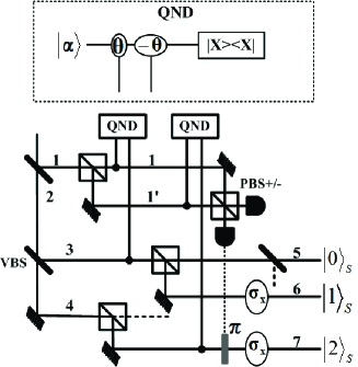
Figure 3: Schematic setup for the transformation with XPM process. Two QND modules working with XPM process are used here. The transformation is realized under the condition that the two qubus beams pick no phase shift, with the corresponding success probability 1/6. For the details, see text.

With weak cross-Kerr nonlinearity, we implement the transformation from a bi-photonic qutrit to a single photon qutrit as shown in Fig. 3. An initial bi-photonic qutrit in the state $\left|\psi\right\rangle_{in}$ of Eq. (1) is first sent to a 50:50 BS, making the following transformation

$$\left(\frac{\alpha}{\sqrt{2}}a_{H}^{\dagger 2}+\beta a_{H}^{\dagger}a_{V}^{\dagger}+\frac{\gamma}{\sqrt{2}}a_{V}^{\dagger 2}\right)\left|vac\right\rangle$$

$$\rightarrow\left[\frac{\alpha}{2\sqrt{2}}\left(a_{H1}^{\dagger}+a_{H2}^{\dagger}\right)^{2}+\frac{\beta}{2}\left(a_{H1}^{\dagger}+a_{H2}^{\dagger}\right)\right.$$

$$\left.\times\left(a_{V1}^{\dagger}+a_{V2}^{\dagger}\right)+\frac{\gamma}{2\sqrt{2}}\left(a_{V1}^{\dagger}+a_{V2}^{\dagger}\right)^{2}\right]\left|vac\right\rangle.$$ (17)

Next a VBS is placed on path 2 such that

$$a_{H2}^{\dagger} \rightarrow ra_{H3}^{\dagger}+ta_{H4}^{\dagger},$$

$$a_{V2}^{\dagger} \rightarrow ra_{V3}^{\dagger}+ta_{V4}^{\dagger}.$$ (18)

Then, after three PBSs change the spatial modes as $1\rightarrow 1,1^{\prime}$, $3\rightarrow 5,6$, $4\rightarrow 7$, two qubus beams (i.e. coherent states) $\left|\alpha_{1}\right\rangle\left|\alpha_{2}\right\rangle$ will be coupled to the corresponding photonic modes through the XPM processes in two quantum nondemolition detection (QND) modules, which are shown in dashed line of Fig. 3. The result will be the following transformation of the total system:

$$\left(\frac{\alpha}{\sqrt{2}}ra_{H1}^{\dagger}a_{H5}^{\dagger}+\frac{\beta}{2}ra_{H1}^{\dagger}a_{V6}^{\dagger}+\frac{\gamma}{\sqrt{2}}ta_{V1^{\prime}}^{\dagger}a_{V7}^{\dagger}\right)\left|vac\right\rangle$$

$$\times\left|\alpha_{1}\right\rangle\left|\alpha_{2}\right\rangle+rest.,$$ (19)

where we only give the terms that two qubus beams pick no phase shift. These terms can be separated from the others by the quadrature measurement $\left|X\right\rangle\left\langle X\right|$, which is implementable with homodyne-heterodyne measurement Nemoto ; Spiller , to obtain the following state

$$\left(\frac{\alpha}{\sqrt{2}}ra_{H1}^{\dagger}a_{H5}^{\dagger}+\frac{\beta}{2}ra_{H1}^{\dagger}a_{V6}^{\dagger}+\frac{\gamma}{\sqrt{2}}ta_{V1^{\prime}}^{\dagger}a_{V7}^{\dagger}\right)\left|vac\right\rangle$$

$$=\frac{\alpha}{\sqrt{2}}r\left|H\right\rangle_{1}\left|H\right\rangle_{5}+\frac{\beta}{2}r\left|H\right\rangle_{1}\left|V\right\rangle_{6}+\frac{\gamma}{\sqrt{2}}t\left|V\right\rangle_{1}\left|V\right\rangle_{7}.$$ (20)

This state can be expressed as

$$\frac{\alpha}{2}r\left(\left|+\right\rangle_{1}+\left|-\right\rangle_{1}\right)\left|H\right\rangle_{5}+\frac{\beta}{2\sqrt{2}}r\left(\left|+\right\rangle_{1}+\left|-\right\rangle_{1}\right)\left|V\right\rangle_{6}$$

$$+\frac{\gamma}{2}t\left(\left|+\right\rangle_{1}-\left|-\right\rangle_{1}\right)\left|V\right\rangle_{7},$$ (21)

where $\left|\pm\right\rangle=\frac{1}{\sqrt{2}}\left(\left|H\right\rangle+\left|V\right\rangle\right)$. Now, we use a PBS_± which transmits $\left|+\right\rangle$ and reflects $\left|-\right\rangle$, and the following two photon number non-resolving detectors. If the detection is $\left|+\right\rangle$, the state

$$\frac{\alpha}{\sqrt{2}}r\left|H\right\rangle_{5}+\frac{\beta}{2}r\left|V\right\rangle_{6}+\frac{\gamma}{\sqrt{2}}t\left|V\right\rangle_{7}$$ (22)

will be projected out; on the other hand, if the detection is $\left|-\right\rangle$, what is realized is

$$\frac{\alpha}{\sqrt{2}}r\left|H\right\rangle_{5}+\frac{\beta}{2}r\left|V\right\rangle_{6}-\frac{\gamma}{\sqrt{2}}t\left|V\right\rangle_{7},$$ (23)

which can be transform to the state in Eq. (22) by the conditional phase shifter $\pi$ on path 7. By selecting $\frac{r}{2}=\frac{t}{\sqrt{2}}$, i.e., $t=\frac{1}{\sqrt{3}}$, and using a 50:50 BS for the mode 5 and two $\sigma_{x}$ operations for modes 6, 7, we can achieve the following state,

$$\frac{1}{\sqrt{6}}\left(\alpha\left|H\right\rangle_{5}+\beta\left|H\right\rangle_{6}+\gamma\left|H\right\rangle_{7}\right),$$ (24)

which is the single photon qutrit $\left|\psi\right\rangle_{S}$ in Eq. (2). The success probability is $\frac{1}{6}$, which is much higher than that of the linear optical scheme. Moreover, no ancilla single photon is necessary here.

The scheme is based on quadrature projection after XPM process, so it does not require any post-selection by coincidence measurement. But it needs an XPM phase shift of $-\theta$, which is only possible with the equivalent phase shift $2\pi-\theta$ and could be impractical Kok . The XPM phase shift $\theta\sim 10^{-2}$ is possible with, for example, electromagnetically induced transparencies (EIT) EIT , whispering-gallery microresonators WGM , optical fibers OF , or cavity QED systems QED , but the corresponding $2\pi-\theta$ will be too large to realize by the available techniques. To avoid the XPM phase shift of $-\theta$, we propose a different design of the transformation shown in Fig. 4. Here we use the double XPM method in He to replace the two XPM processes without changing anything else.

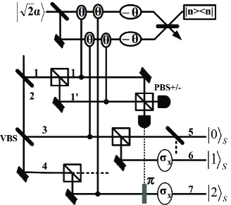
Figure 4: Schematic setup for the transformation from bi-photon qutrits to the corresponding single photon qutrits with double XPM method. The only difference from Fig. 3 is that the two separate XPM processes are replaced by a double XPM process of two identical qubus beams. In the design, no XPM phase shift of $-\theta$ will be necessary, and it makes the scheme more feasible.

We describe it briefly as the process is similar. In the double XPM process two qubus beams $\left|\alpha\right\rangle\left|\alpha\right\rangle$ will be coupled to the corresponding photonic modes as shown in Fig. 4. The XPM pattern in Fig. 4 is that the first beam being coupled to the $\left|H\right\rangle$ mode on path 1 and the $\left|V\right\rangle$ mode on path 4, while the second beam to $\left|V\right\rangle$ mode on path $1^{\prime}$ and the modes on path 3. Suppose the XPM phase shifts induced by the couplings are all $\theta$. After that, the total system will be transformed to

$$\left(\frac{\alpha}{\sqrt{2}}ra_{H1}^{\dagger}a_{H3}^{\dagger}+\frac{\beta}{2}a_{H1}^{\dagger}a_{V1^{\prime}}^{\dagger}+\frac{\beta}{2}ra_{H1}^{\dagger}a_{V3}^{\dagger}\right.$$

$$\left.+\frac{\beta}{2}rta_{H3}^{\dagger}a_{V4}^{\dagger}+\frac{\gamma}{2\sqrt{2}}ta_{V1}^{\dagger}a_{V4}^{\dagger}+\frac{\gamma}{2\sqrt{2}}rta_{V3}^{\dagger}a_{V4}^{\dagger}\right)$$

$$\times\left|vac\right\rangle\left|\alpha e^{i\theta}\right\rangle\left|\alpha e^{i\theta}\right\rangle+\frac{\alpha}{2\sqrt{2}}t^{2}a_{H4}^{\dagger 2}\left|vac\right\rangle\left|\alpha\right\rangle\left|\alpha\right\rangle+rest.,$$ (25)

where $rest.$ denotes the terms that the two qubus beams pick up the different phase shifts. A phase shifter of $-\theta$ is respectively applied to two qubus beams, and then one more 50:50 BS implements the transformation $\left|\alpha_{1}\right\rangle\left|\alpha_{2}\right\rangle\rightarrow\left|\frac{\alpha_{1}-\alpha_{2}}{\sqrt{2}}\right\rangle\left|\frac{\alpha_{1}+\alpha_{2}}{\sqrt{2}}\right\rangle$ of the coherent-state components. The above state will be therefore transformed to

$$\left(\frac{\alpha}{\sqrt{2}}ra_{H1}^{\dagger}a_{H3}^{\dagger}+\frac{\beta}{2}a_{H1}^{\dagger}a_{V1^{\prime}}^{\dagger}+\frac{\beta}{2}ra_{H1}^{\dagger}a_{V3}^{\dagger}\right.$$

$$\left.+\frac{\beta}{2}rta_{H3}^{\dagger}a_{V4}^{\dagger}+\frac{\gamma}{2\sqrt{2}}ta_{V1}^{\dagger}a_{V4}^{\dagger}+\frac{\gamma}{2\sqrt{2}}rta_{V3}^{\dagger}a_{V4}^{\dagger}\right)$$

$$\times\left|vac\right\rangle\left|0\right\rangle\left|\sqrt{2}\alpha\right\rangle+\frac{\alpha}{2\sqrt{2}}t^{2}a_{H4}^{\dagger 2}\left|vac\right\rangle\left|0\right\rangle\left|\sqrt{2}\alpha\right\rangle+rest.$$ (26)

Then, we could use the projections $\left|n\right\rangle\left\langle n\right|$ on the first qubus beam to get the proper output. If $n=0$, and by the post-selection that one photon will appear on the output (5, 6, 7) while a click on one of the two detectors after the PBS_±, the state in Eq. (20) can be therefore projected out. Similar to the process in Fig. 3, we can achieve the final single photon qutrit $\left|\psi\right\rangle_{S}$ with the success probability $\frac{1}{6}.$ Though this design requires the post-selection, it dispenses with the XPM phase shift of $-\theta$, so it could be more experimentally feasible.

III.2 Inverse transformation with XPM process

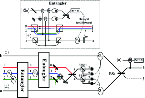
Figure 5: Schematic setup for the inverse transformation with XPM process. The part called Entangler shown in dashed line entangles the single photon qutrit and the ancilla single photon. Out of the Entangler, the polarization of the ancilla photon will be the same as those of the single photon qutrit. This inverse transformation can be implemented with a success probability 1/2.

Now we should transform the output single photon qutrit back to a bi-photonic qutrit. We apply the inverse transformation procedure shown in Fig. 5, and will show that it can be realized with a success probability as high as $\frac{1}{2}$.

At first, we apply a setup called Entangler shown in dashed line to the transformed single photon qutrit $\left|\psi^{{}^{\prime}}\right\rangle_{S}=\alpha^{{}^{\prime}}\left|H\right\rangle_{0}+\beta^{{}^{\prime}}\left|H\right\rangle_{1}+\gamma^{{}^{\prime}}\left|H\right\rangle_{2}$ with an ancilla single photon in the state $\left|\pm\right\rangle_{a}$, after a $\sigma_{x}$ operation performed on the spatial modes $1$, $2$, respectively. The Entangler is to implement the transformation,

$$\left|\psi^{{}^{\prime}}\right\rangle_{S}\left|+\right\rangle_{a}\rightarrow\alpha^{{}^{\prime}}\left|HH\right\rangle_{0,a}+\beta^{{}^{\prime}}\left|VV\right\rangle_{1,a}+\gamma^{{}^{\prime}}\left|VV\right\rangle_{2,a},$$ (27)

where the polarization of the ancilla single photon will be the same as that of the single photon qutrit. In the Entangler, two qubus beams $\left|\alpha\right\rangle\left|\alpha\right\rangle$ are introduced, and then coupled to the corresponding photonic modes through the XPM processes. The XPM pattern in Fig. 5 is that the first beam being coupled to $\left|V\right\rangle$ modes on path 1, 2 and the $\left|H\right\rangle$ mode of the ancilla photon, while the second beam to $\left|H\right\rangle$ mode on path 0 and the $\left|V\right\rangle$ mode of the ancilla photon. Suppose the XPM phase shifts induced by the couplings are all $\theta$. As the result, we will transform the total system to

$$\frac{1}{\sqrt{2}}\left(\alpha^{{}^{\prime}}\left|HH\right\rangle_{0,a}+\beta^{{}^{\prime}}\left|VV\right\rangle_{1,a}+\gamma^{{}^{\prime}}\left|VV\right\rangle_{2,a}\right)\left|\alpha e^{i\theta}\right\rangle\left|\alpha e^{i\theta}\right\rangle$$

$$+\frac{1}{\sqrt{2}}\alpha^{{}^{\prime}}\left|HV\right\rangle_{0,a}\left|\alpha\right\rangle\left|\alpha e^{i2\theta}\right\rangle$$

$$+\frac{1}{\sqrt{2}}\left(\beta^{{}^{\prime}}\left|VH\right\rangle_{1,a}+\gamma^{{}^{\prime}}\left|VH\right\rangle_{2,a}\right)\left|\alpha e^{i2\theta}\right\rangle\left|\alpha\right\rangle.$$ (28)

After that, a phase shifter of $-\theta$ is respectively applied to two qubus beams, and then one more 50:50 BS implements the transformation $\left|\alpha_{1}\right\rangle\left|\alpha_{2}\right\rangle\rightarrow\left|\frac{\alpha_{1}-\alpha_{2}}{\sqrt{2}}\right\rangle\left|\frac{\alpha_{1}+\alpha_{2}}{\sqrt{2}}\right\rangle$ of the coherent-state components. The state of the total system will be therefore transformed to

$$\frac{1}{\sqrt{2}}\left(\alpha^{{}^{\prime}}\left|HH\right\rangle_{0,a}+\beta^{{}^{\prime}}\left|VV\right\rangle_{1,a}+\gamma^{{}^{\prime}}\left|VV\right\rangle_{2,a}\right)\left|0\right\rangle\left|\sqrt{2}\alpha\right\rangle$$

$$+\frac{1}{\sqrt{2}}\alpha^{{}^{\prime}}\left|HV\right\rangle_{0,a}\left|-i\sqrt{2}\alpha\sin\theta\right\rangle\left|\sqrt{2}\alpha\cos\theta\right\rangle$$

$$+\frac{1}{\sqrt{2}}\left(\beta^{{}^{\prime}}\left|VH\right\rangle_{1,a}+\gamma^{{}^{\prime}}\left|VH\right\rangle_{2,a}\right)\left|i\sqrt{2}\alpha\sin\theta\right\rangle\left|\sqrt{2}\alpha\cos\theta\right\rangle.$$ (29)

The first coherent-state component in Eq. (29) is either vacuum or a cat state (the superposition of $\left|\pm i\sqrt{2}\alpha\sin\theta\right\rangle$ in the second piece). The target output could be therefore obtained by the projection $\left|n\right\rangle\left\langle n\right|$ on the first qubus beam. If $n=0$, we will obtain

$$\alpha^{{}^{\prime}}\left|HH\right\rangle_{0,a}+\beta^{{}^{\prime}}\left|VV\right\rangle_{1,a}+\gamma^{{}^{\prime}}\left|VV\right\rangle_{2,a},$$ (30)

with the polarization of ancilla photon the same to the single photon qutrit. If $n\neq 0$, on the other hand, there will be the output

$$e^{-in\frac{\pi}{2}}\alpha^{{}^{\prime}}\left|HV\right\rangle_{0,a}+e^{in\frac{\pi}{2}}\left(\beta^{{}^{\prime}}\left|VV\right\rangle_{1,a}+\gamma^{{}^{\prime}}\left|VV\right\rangle_{2,a}\right),$$ (31)

which can be transformed to the form in Eq. (30) by a phase shift $\pi$ following the classically feed-forwarded measurement result $n$ and a $\sigma_{x}$ operation on the ancilla photon.

Next, the second Entangler will be applied to the above output and another ancilla single photon $\left|\pm\right\rangle_{b}$, after a $\sigma_{x}$ operation is performed on spatial mode $1$. In this Entangler, the transmitted path for mode 1 is now active while the reflected port is only active in the first Entangler. Similar to the first Entangler, the second implements the transformation

$$\left(\alpha^{{}^{\prime}}\left|HH\right\rangle_{0,a}+\beta^{{}^{\prime}}\left|HV\right\rangle_{1,a}+\gamma^{{}^{\prime}}\left|VV\right\rangle_{2,a}\right)\left|+\right\rangle_{b}$$

$$\rightarrow\alpha^{{}^{\prime}}\left|HHH\right\rangle_{0,a,b}+\beta^{{}^{\prime}}\left|HVH\right\rangle_{1,a,b}+\gamma^{{}^{\prime}}\left|VVV\right\rangle_{2,a,b}.$$ (32)

Also we need to erase the path information of the first photon. We first combine the modes 1 and 2 by a PBS, and then make them interfere with the mode 0 through a 50:50 BS to achieve the following state

$$\frac{\alpha^{{}^{\prime}}}{\sqrt{2}}\left(\left|H\right\rangle_{3}+\left|H\right\rangle_{4}\right)\left|HH\right\rangle_{a,b}+\frac{\beta^{{}^{\prime}}}{\sqrt{2}}\left(\left|H\right\rangle_{3}-\left|H\right\rangle_{4}\right)\left|VH\right\rangle_{a,b}$$

$$+\frac{\gamma^{{}^{\prime}}}{\sqrt{2}}\left(\left|V\right\rangle_{3}-\left|V\right\rangle_{4}\right)\left|VV\right\rangle_{a,b}.$$ (33)

By two PBS_±, the state

$$\frac{1}{2}\left(\alpha^{{}^{\prime}}\left|HH\right\rangle_{a,b}+\beta^{{}^{\prime}}\left|VH\right\rangle_{a,b}+\gamma^{{}^{\prime}}\left|VV\right\rangle_{a,b}\right)\left|+\right\rangle_{5}$$

$$+\frac{1}{2}\left(\alpha^{{}^{\prime}}\left|HH\right\rangle_{a,b}+\beta^{{}^{\prime}}\left|VH\right\rangle_{a,b}-\gamma^{{}^{\prime}}\left|VV\right\rangle_{a,b}\right)\left|-\right\rangle_{6}$$

$$+\frac{1}{2}\left(\alpha^{{}^{\prime}}\left|HH\right\rangle_{a,b}-\beta^{{}^{\prime}}\left|VH\right\rangle_{a,b}-\gamma^{{}^{\prime}}\left|VV\right\rangle_{a,b}\right)\left|+\right\rangle_{7}$$

$$+\frac{1}{2}\left(\alpha^{{}^{\prime}}\left|HH\right\rangle_{a,b}-\beta^{{}^{\prime}}\left|VH\right\rangle_{a,b}+\gamma^{{}^{\prime}}\left|VV\right\rangle_{a,b}\right)\left|-\right\rangle_{8}$$ (34)

will be then obtained. With four detectors on path 5, 6, 7 and 8, as well as the classical feedforward, the state

$$\alpha^{{}^{\prime}}\left|HH\right\rangle_{a,b}+\beta^{{}^{\prime}}\left|VH\right\rangle_{a,b}+\gamma^{{}^{\prime}}\left|VV\right\rangle_{a,b},$$ (35)

will be finally realized. The above processes could be deterministic.

The final step is to merge the two photons into the same spatial mode, which could be simply realized by a BS and the following QND module. In this QND module, a qubus beam $\left|\alpha\right\rangle$ will be coupled to one of the output modes of BS₁. After that, the state in Eq. (35) plus the qubus beam will evolve to

$$\frac{1}{\sqrt{2}}\left(\alpha^{{}^{\prime}}\left|HH\right\rangle_{1,1}+\frac{1}{\sqrt{2}}\beta^{{}^{\prime}}\left|VH\right\rangle_{1,1}+\gamma^{{}^{\prime}}\left|VV\right\rangle_{1,1}\right)\left|\alpha e^{i2\theta}\right\rangle$$

$$+\frac{1}{\sqrt{2}}\beta^{{}^{\prime}}\left(\left|VH\right\rangle_{1,2}+\left|VH\right\rangle_{2,1}\right)\left|\alpha e^{i\theta}\right\rangle$$

$$+\frac{1}{\sqrt{2}}\left(\alpha^{{}^{\prime}}\left|HH\right\rangle_{2,2}+\frac{1}{\sqrt{2}}\beta^{{}^{\prime}}\left|VH\right\rangle_{2,2}+\gamma^{{}^{\prime}}\left|VV\right\rangle_{2,2}\right)\left|\alpha\right\rangle.$$ (36)

Through the quadrature measurement $\left|X\right\rangle\left\langle X\right|$, the following state

$$\alpha^{{}^{\prime}}\left|HH\right\rangle_{1,1}+\frac{1}{\sqrt{2}}\beta^{{}^{\prime}}\left|VH\right\rangle_{1,1}+\gamma^{{}^{\prime}}\left|VV\right\rangle_{1,1}$$ (37)

or

$$\alpha^{{}^{\prime}}\left|HH\right\rangle_{2,2}+\frac{1}{\sqrt{2}}\beta^{{}^{\prime}}\left|VH\right\rangle_{2,2}+\gamma^{{}^{\prime}}\left|VV\right\rangle_{2,2}$$ (38)

can be selected out, and the output with only one photon at each output port, which picks up the phase shift $\theta$ in the XPM process, will be discarded. The different coefficients between the mid term and the other two terms in Eqs. (37) and (38) are caused by the Hong-Ou-Mandal (HOM) interference effect on BS₁. In order to balance the coefficients, we should use a 50:50 BS respectively on path 0 and 2 (see Fig. 5). After that we could achieve the bi-photonic qutrit $\alpha^{{}^{\prime}}\left|0\right\rangle_{3}+\beta^{{}^{\prime}}\left|1\right\rangle_{3}+\gamma^{{}^{\prime}}\left|2\right\rangle_{3}$ with the success probability $\frac{1}{2}$, and then the total success probability for an arbitrary unitary operation on biphoton qutrits will be $\frac{1}{6}\times\frac{1}{2}=\frac{1}{12}$.

IV Discussion

We have presented two schemes for unitary operations on biphoton qutrits, which are realized through bi-directional mapping between polarization and spatially encoded photonic qutrits. Through the bi-directional mapping any unitary operation $U(3)$ on bi-photonic qutrits can be reduced to that on single photon qutrits. The linear optical scheme succeeds with a small probability $1.17\times 10^{-4}$, but it can be increased to $1/12$ with weak cross-Kerr nonlinearity. The probabilistic nature of the schemes is due to the two indistinguishable photons in the same spatial-temporal modes. For example, at the last merging step in Fig. 5, the probability to get the proper output state will be lowered by $1/2$ because of the HOM interference.

Finally, we look at the feasibility of the schemes. The first scheme applies common experimental tools such as linear optical circuits, coincidence measurements, and detection with APDs. The difficulty in the implementation is the accuracy for the numerous interferences between the photonic modes. The additional requirement in the second scheme is the good performance of weak cross-Kerr nonlinearity. The error in each XPM process can be effectively eliminated under the condition $\alpha\theta\gg 1$ Spiller , which means that the small XPM phase $\theta$ can be compensated by the large amplitude $|\alpha|$ of the qubus or communication beams. The other advantage of the scheme based on weak nonlinearity is the fewer ancilla photons—the ancilla photons are only required in the inverse transformation. This could make the experimental implementation more simplified.

- (1) N. K. Langford et al., Phys. Rev. Lett. 93, 053601 (2004); R.W. Spekkens and T. Rudolph, Phys. Rev. A 65, 012310 (2001); G. Molina-Terriza et al., Phys. Rev. Lett. 92, 167903 (2004); S. Grölacher et al., New J. Phys. 8, 75 (2006); D. Bruß and C. Macchiavello, Phys. Rev. Lett. 88, 127901 (2002); N. J. Cerf et al., Phys. Rev. Lett. 88, 127902 (2002); T. Durt et al., Phys. Rev. A 67, 012311 (2003).
- (2) T. C. Ralph, K. Resch, A. Gilchrist, Phys. Rev. A 75, 022313 (2007); B. P. Lanyon, et al., Nature Physics 5, 134-140 (2009).
- (3) A. Mair et al, Nature (London) 412, 313 (2001); A. Vaziri et al, Phys. Rev. Lett. 89, 240401 (2002).
- (4) L. Neves et al, Phys. Rev. A 69, 042305 (2004); L. Neves et al, Phys. Rev. Lett. 94, 100501 (2005); M. N. O’Sullivan-Hale et al, Phys. Rev. Lett. 94, 220501 (2005).
- (5) R. T. Thew et al, Phys. Rev. Lett. 93, 010503 (2004); H. de Riedmatten et al, Phys. Rev. A 69, 050304(R) (2004).
- (6) J. C. Howell et al, Phys. Rev. Lett. 88, 030401 (2002); Y.I. Bogdanov et al, Phys. Rev. Lett. 93, 230503 (2004); E. V. Moreva et al, Phys. Rev. Lett. 97, 023602 (2006); G. Vallone et al, Phys. Rev. A 76, 012319 (2007); Y. M. Li et al, Phys. Rev. A 77, 015802 (2008).
- (7) H. Mikami and T. Kobayashi, Phys. Rev. A, 75, 022325 (2007).
- (8) B. P. Lanyon, T. J. Weinhold, N. K. Langford, J. L. O’Brien, K. J. Resch, A. Gilchrist, and A. G. White, Phys. Rev. Lett. 100, 060504 (2008).
- (9) If we adopt the notation , , in Lanyon , there will be no difference from the results obtained in the present paper, since any input in this basis can be represented as , where refers to the permutation of two indistinguishable photons, and is the qutrit defined in the logic basis of Eq. (1).
- (10) Y. I. Bogdanov et al., Phys. Rev. A 70, 042303 (2004).
- (11) M. Reck, A. Zeilinger, H. J. Bernstein and P. Bertani, Phys. Rev. Lett. 73, 58 (1994).
- (12) C. K. Hong, Z. Y. Ou, and L. Mandel, Phys. Rev. Lett. 59, 2044 (1987).
- (13) M. A. Nielsen and I. L. Chuang, Quantum Computation and Quantum Information (Cambridge University Press, Cambridge, 2000).
- (14) S. D. Barrett, P. Kok, K. Nemoto, R. G. Beausoleil, W. J. Munro, and T. P. Spiller, Phys. Rev. A 71, 060302(R) (2005).
- (15) K. Nemoto and W. J. Munro, Phys. Rev. Lett. 93, 250502 (2004).
- (16) W. J. Munro, K. Nemoto and T. P. Spiller, New J. Phys. 7, 137 (2005); T. P. Spiller, K. Nemoto, S. L. Braunstein, W. J. Munro, P. van Loock and G. J. Milburn, New J. Phys. 8, 30 (2006).
- (17) Q. Lin and J. Li, Phys. Rev. A, 79, 022301 (2009).
- (18) B. He, Y.-H. Ren, and J. A. Bergou, Phys. Rev. A 79, 052323 (2009).
- (19) P. Kok, Phys. Rev. A 77, 013808 (2008).
- (20) S. E. Harris and L. V. Hau, Phys. Rev. Lett. 82, 4611 (1999); W. J. Munro, Kae Nemoto, R. G. Beausoleil, and T. P. Spiller, Phys. Rev. A 71, 033819 (2005); D. A. Braje et al., Phys. Rev. A 68, 041801(R) (2003).
- (21) T. J. Kippenberg, S. M. Spillane, and K. J. Vahala, Phys. Rev. Lett. 93, 083904 (2004).
- (22) X. Li, P. L. Voss, J. E. Sharping, and P. Kumar, Phys. Rev. Lett. 94, 053601 (2005).
- (23) P. Grangier, J. A. Levenson, and J.-P. Poizat, Nature (London) 369, 537 (1998); Q. A. Turchette et al., Phys. Rev. Lett. 75, 4710 (1995).