Distortion of the HBT images by meson clouds

Abstract

We study the effects of mesonic final state interactions on the Hanbury Brown and Twiss (HBT) intensity interferometry for mesons in ultra-relativistic heavy ion collisions. Modification of the one-body amplitude of emitted mesons while going through a cloud of other mesons is estimated in the semiclassical approximation with a mesonic optical potential which incorporates both coherent forward scattering with other mesons and the absorption due to the incoherent scattering in the meson clouds. We show how these effects results in the distortion of the HBT images.

Hanbury Brown and Twiss intensity interferometry, originally developed in radio astronomy to measure stellar radii[1], and later played a seminal role in the development of quantum optics[2], has been applied to measure the source size of the secondary particles emitted in high energy heavy ion collisions.[3, 4, 5] Recent analysis of the RHIC experiments has shown that the source shape determined from the data has a systematic deviation from the prediction of the hydrodynamical models [6, 7, 8, 9]: this has been called ”RHIC HBT puzzle”.

The HBT formula for the correlation function usually used in data analysis assumes: [12] 1) random initial phases (incoherent source), 2) factorization of two-point source function, 3) neglection of all the interaction between two detected pions and the rest of the system after the emission. Each of these underlying assumptions may need to be checked in order to find a resolution of the ”HBT puzzle”. In this work, we investigate the effects of the final state interactions on the correlation function, assuming the first two assumptions are valid.

We focus on the effect of one-body interaction, namely the interacion between each of the observed pairs and rest of the system via mean field potential. The mutual interaction between the two detected pions is dominated at large separation, corresponding to small $q$, by long range Coulomb interaction, rather than strong interaction, and such effect has been incorporated by the well-known Gamow factor in the correlation function[4]. In the usual hydrodynamical modeling, the particle momenta are considered to be frozen on the kinetic freeze-out surface. In the kinetic theoretical language, this implies that the collisions between two particles which maintains the system in local equilibrium becomes suddenly ineffective. However, there still remains interaction between each of the pair and the evaporating particles in the vicinity of the emission points. We introduce mesonic optical potential to describe such effects: the real part of the potential describes a coherent forward scattering of the particle with the other mesons, while the imaginary absorptive part incorporates the effect of incoherent scattering with other individual mesons. We examine how extracted HBT images are distorted due to the modification of the one-body amplitudes in the mesonic optical potential.

In the standard picture of ultrarelativistic nuclear collisions, the pion source extends along the direction of the motion of colliding nuclei in an approximately boost invariant fashion[13]. We follow this picture, together with cylindrical symmetry of the collision volume, and concentrate on the quantum evolution of a group of particles appearing in a small central rapidity bin $-\frac{1}{2}\Delta y<y<\frac{1}{2}\Delta y$ on the two-dimensional transverse plane in their center-of-mass frame.

Two particle momentum correlation function of identical particle which we are concerned is given by

$$C(\bm{k}_{1},\bm{k}_{2})=\frac{P_{2}(\bm{k}_{1},\bm{k}_{2})}{P_{1}(\bm{k}_{1})P_{1}(\bm{k}_{2})}$$ (1)

where $P_{2}(\bm{k}_{1},\bm{k}_{2})$ is the joint probability of detecting a pair of the same kind of pions with momenta $\bm{k}_{1}$ and $\bm{k}_{2}$, and $P_{1}(\bm{k})$ is the probability for a detection of single pion. They may be given in terms of the asymptotic form of the matrix elements of the density matrix: $P_{1}(\bm{k})=\langle\bm{k}|\hat{\rho}(\infty)|\bm{k}\rangle$ , $P_{2}(\bm{k}_{1},\bm{k}_{2})=\langle\bm{k}_{1}\bm{k}_{2}|\hat{\rho}(\infty)|\bm{k}_{1}\bm{k}_{2}\rangle$. Here we adopt the Schrödinger picture in which the time evolution of the density matrix is given by $\hat{\rho}(t)=U(t)\hat{\rho}(0)U^{\dagger}(t)$ so that we may write

$$P_{1}(\bm{k}) = \lim_{t\to\infty}\int d\bm{x}_{1}d\bm{x}_{2}\langle\bm{k}|U(t)|\bm{x}_{1}\rangle\langle\bm{x}_{1}|\hat{\rho}(0)|\bm{x}_{2}\rangle\langle\bm{x}_{2}|U^{\dagger}(t)|\bm{k}\rangle\ ,$$ (2)

$$= \lim_{t\to\infty}\int d\bm{x}_{1}d\bm{x}_{2}\varphi_{\bm{k}}(\bm{x}_{1},t)\rho_{0}(\bm{x}_{1},\bm{x}_{2})\varphi^{*}_{\bm{k}}(\bm{x}_{2},t)$$

$$P_{2}(\bm{k}_{1},\bm{k}_{2}) = \lim_{t\to\infty}\int\!\!d\bm{x}_{1}d\bm{x}_{2}d\bm{x}^{\prime}_{1}d\bm{x}^{\prime}_{2}\langle\bm{k}_{1}\bm{k}_{2}|U(t)|\bm{x}_{1}\bm{x}_{1}^{\prime}\rangle$$

$$\qquad\qquad\qquad\times\langle\bm{x}_{1},\bm{x}_{2}|\hat{\rho}(0)|\bm{x}^{\prime}_{1},\bm{x}^{\prime}_{2}\rangle\langle\bm{x}_{2}\bm{x}^{\prime}_{2}|U^{\dagger}(t)|\bm{k}_{1}\bm{k}_{2}\rangle$$

$$= \lim_{t\to\infty}\int d\bm{x_{1}}d\bm{x_{2}}d\bm{x}^{\prime}_{1}d\bm{x}^{\prime}_{2}\Psi_{\bm{k}_{1},\bm{k}_{2}}(\bm{x}_{1},\bm{x}_{2};t)\rho_{0}(\bm{x_{1}},\bm{x_{2}};\bm{x}^{\prime}_{1},\bm{x}^{\prime}_{2})\Psi^{*}_{\bm{k}_{1},\bm{k}_{2}}(\bm{x}^{\prime}_{1},\bm{x}^{\prime}_{2},t)$$

where $\varphi_{\bm{k}}(\bm{x},t)=\langle\bm{k}|U(t)|\bm{x}\rangle$ is the amplitude that a particle emitted at $\bm{x}$ is detected with momentum $\bm{k}$ at time $t$, while $\Psi_{\bm{k}_{1},\bm{k}_{2}}(\bm{x}_{1},\bm{x}_{2},t)=\langle\bm{k}_{1}\bm{k}_{2}|U(t)|\bm{x}_{1}\bm{x}_{2}\rangle$ is the two-particle amplitude that two particles are emitted at $\bm{x}_{1}$ and $\bm{x}_{2}$ and detected with momenta $\bm{k}_{1}$ and $\bm{k}_{2}$ at time $t$ simultaneously. We have introduced the one-particle reduced density matrix, $\rho_{1}(\bm{x}_{1},\bm{x}_{2})=\langle\bm{x}_{1}|\hat{\rho}(0)|\bm{x}_{2}\rangle$, and the two particle reduced density matrix, $\rho_{2}(\bm{x}_{1},\bm{x}_{2};\bm{x}^{\prime}_{1},\bm{x}^{\prime}_{2})=\langle\bm{x}_{1},\bm{x}_{2}|\hat{\rho}(0)|\bm{x}^{\prime}_{1},\bm{x}^{\prime}_{2}\rangle$ which obey, due to the bosonic symmetry of the two particle states ($|\bm{x}_{1},\bm{x}_{2}\rangle=|\bm{x}_{2},\bm{x}_{1}\rangle$) ,

$$\rho_{2}(\bm{x}_{1},\bm{x}_{2};\bm{x}^{\prime}_{1},\bm{x}^{\prime}_{2})=\rho_{2}(\bm{x}_{2},\bm{x}_{1};\bm{x}^{\prime}_{1},\bm{x}^{\prime}_{2})=\rho_{2}(\bm{x}_{1},\bm{x}_{2};\bm{x}^{\prime}_{2},\bm{x}^{\prime}_{1})$$ (4)

The basic objective of the HBT interferometry is to extract information of the density matrix from the observed correlation function $C(\bm{k}_{1},\bm{k}_{2})$.

If the particles do not interact after $t=0$, the time evolution operator turns into a trivial phase factor and the single particle amplitude becomes just a plane wave: $\langle\bm{k}|e^{-i\hat{H}t}|\bm{x}\rangle=e^{-iE_{k}t}\langle\bm{k}|\bm{x}\rangle=e^{-i(\bm{k}\cdot\bm{x}+E_{k}t)}$. This results in

$$P_{1}(\bm{k}) = \int d\bm{x}_{1}d\bm{x}_{2}\rho_{0}(\bm{x}_{1},\bm{x}_{2})e^{-i\bm{k}\cdot(\bm{x}_{1}-\bm{x}_{2})}=\int\!\!d\bm{x}\ f(\bm{x},\bm{k})$$ (5)

where $f(\bm{x},\bm{k})$ with $\bm{x}=(\bm{x}_{1}+\bm{x}_{2})/2$ is the one-body phase space distribution function or the Wigner function at $t=0$. Similarly, in the absence of the final state interaction, the symmetrized two particle amplitude becomes, $\langle\bm{k}_{1}\bm{k}_{2}|U(t)|\bm{x}_{1}\bm{x}_{2}\rangle=\frac{1}{\sqrt{2}}\left[e^{-i(\bm{k}_{1}\cdot\bm{x}_{1}+\bm{k}_{2}\cdot\bm{x}_{2})}+e^{-i(\bm{k}_{1}\cdot\bm{x}_{2}+\bm{k}_{2}\cdot\bm{x}_{1})}\right]e^{-i(E_{1}+E_{2})t}$. If we insert this expression into Eq (LABEL:eq:P2a) and further assume the factorization of the two particle density matrix, $\rho_{0}(\bm{x_{1}},\bm{x_{2}};\bm{x}^{\prime}_{1},\bm{x}^{\prime}_{2})=\frac{1}{2}\left[\rho_{0}(\bm{x}_{1},\bm{x}^{\prime}_{1})\rho_{0}(\bm{x}_{2},\bm{x}^{\prime}_{2})+\rho_{0}(\bm{x}_{2},\bm{x}^{\prime}_{1})\rho_{0}(\bm{x}_{1},\bm{x}^{\prime}_{2})\right]$, along with the symmetry (4), we find

$$P_{2}(\bm{k}_{1},\bm{k}_{2})=P_{1}(\bm{k}_{1})P_{1}(\bm{k}_{2})+\left|\int d\bm{x}f(\bm{x},\bar{\bm{k}})e^{i\bm{q}\cdot\bm{x}}\right|^{2}$$ (6)

with $\bar{\bm{k}}=\frac{1}{2}(\bm{k}_{1}+\bm{k}_{2})$ and $\bm{q}=\bm{k}_{1}-\bm{k}_{2}$. For a factorized form of the phase space distribution $f(\bm{x},\bm{k})=\tilde{\rho}(\bm{x})P_{1}(\bm{k})$ with $\int d\bm{x}\tilde{\rho}(\bm{x})=1$, this gives the familiar form of the correlation function,

$$C(\bm{q},\bar{\bm{k}})=1+\eta(\bm{k}_{1},\bm{k}_{2})\left|\int d\bm{x}\tilde{\rho}(\bm{x})e^{i\bm{q}\cdot\bm{x}}\right|^{2},$$ (7)

with a correction factor $\eta(\bm{k}_{1},\bm{k}_{2})=P_{1}^{2}(\bar{\bm{k}})/P_{1}(\bm{k}_{1})P_{1}(\bm{k}_{2})$, which exhibits limiting behaviors: $C(0,\bar{\bm{k}})=2$ and $C(\infty,\bar{\bm{k}})=1$. This formula has been used to reconstruct the source distribution function from the measured two particle momentum correlation. We note that the lesson we learn from this simple exercise is that the phase interference of the symmetrized two-particle amplitude plays essential role to create the two particle momentum correlation.

We now consider how this result is modified in the presence of the final state interaction. We shall study the change of the single particle amplitude $\langle{\bm{k}}|U(t)|{\bm{x}}\rangle$ as well as the two particle amplitude $\langle\bm{k}_{1}\bm{k}_{2}|U(t)|\bm{x}_{1}\bm{x}_{2}\rangle$ by the action of the time evolution operator $U(t)=e^{-i\hat{H}t}$. Here we replace the many-body Hamiltonian $\hat{H}$ by one-body Hamiltonian for a non-relativistic particle propagating in an one-body potential. Without mutual two-body interaction of pion pair, two-body amplitude in (LABEL:eq:P2a) is expressed by the symmetrized products of one-body amplitudes :

$$\langle\bm{k}_{1}\bm{k}_{2}|U(t)|\bm{x}_{1}\bm{x}_{2}\rangle=\frac{1}{2}\left\{\langle\bm{k}_{1}|U(t)|\bm{x}_{1}\rangle\langle\bm{k}_{2}|U(t)|\bm{x}_{2}\rangle+\langle\bm{k}_{1}|U(t)|\bm{x}_{2}\rangle\langle\bm{k}_{2}|U(t)|\bm{x}_{1}\rangle\right\}$$ (8)

We therefore only need to compute the distortion of the single particle amplitude.

We recall that $\varphi_{\bm{k}}({\bm{x}},t)=\langle{\bm{k}}|U(t)|{\bm{x}}\rangle$ denotes the amplitude for a particle emitted at ${\bm{x}}$ at time $t=0$ being detected with asymptotic momentum ${\bm{k}}$ at sufficiently large time $t$. Formally, it may be interpreted as a wave function which obeys the static one-body Schördinger equation on the transverse plane:

$$\left[-\frac{1}{2m}\nabla^{2}+V({\bm{x}})\right]\varphi_{\bm{k}}({\bm{x}},t)=E_{\bm{k}}\varphi_{\bm{k}}({\bm{x}},t)$$ (9)

with $E_{\bm{k}}={\bm{k}}^{2}/2m$. If we assume cylindrical symmetry for the collision volume, this Schrödinger equation in two space dimension may be reduced to a one-dimensional one in a ”central” potential $V(|{\bm{x}}|)$ and may be solved by the standard WKB semiclassical approximation.

Here we adopt more intuitive approach to the problem motivated by the stationary phase approximation of the path integral expression of the amplitude, exploiting an analogy to geometrical optics. We write

$$\langle{\bm{k}}|U(T)|{\bm{x}}\rangle=\int d{\bm{x}}^{\prime}e^{-i{\bm{k}}\cdot{\bm{x}}^{\prime}}\langle{\bm{x}}^{\prime}|U(T)|{\bm{x}}\rangle$$ (10)

and introduce an Ansatz

$$\langle{\bm{x}}^{\prime}|U(T)|{\bm{x}}\rangle\approx A({\bm{x}}^{\prime},{\bm{x}};T)e^{iS_{c}({\bm{x}}^{\prime},T;{\bm{x}},0)}$$ (11)

for the propagator. We work with the classical action integral

$$S_{c}({\bm{x}}_{2},t_{2};{\bm{x}}_{1},t_{1})=\int_{t_{1}}^{t_{2}}dtL({\bm{x}},\dot{{\bm{x}}})$$ (12)

along the classical trajectory $({\bm{x}}(t),{\bm{p}}(t))$ specified by the initial position ${\bm{x}}_{1}$ of the particle at time $t=t_{1}$ and the final position ${\bm{x}}_{2}$ at time $t=t_{2}$. The initial and final momenta of the particle are given by ${\bm{p}}_{1}=-\nabla_{1}S_{c}({\bm{x}}_{2},t_{2};{\bm{x}}_{1},t_{1})$ and ${\bm{p}}_{2}=\nabla_{2}S_{c}({\bm{x}}_{2},t_{2};{\bm{x}}_{1},t_{1})$ with the nablas $\nabla_{1,2}$ operating on ${\bm{x}}_{1,2}$, respectively. For free particle motion

$$S_{c}^{\rm free}({\bm{x}}^{\prime},T;{\bm{x}},0)=\frac{m({\bm{x}}^{\prime}-{\bm{x}})^{2}}{2T}$$ (13)

so that the integration over ${\bm{x}}^{\prime}$, assuming that the prefactor $A({\bm{x}},{\bm{x}}^{\prime},T)$ is a constant, evidently give the previous results: $\langle{\bm{k}}|U(T)|{\bm{x}}\rangle=e^{-i{\bm{k}}\cdot{\bm{x}}-iE_{\bm{k}}T}$. This motivates us to write:

$$\langle{\bm{k}}|U(T)|{\bm{x}}\rangle={\cal A}({\bm{x}},{\bm{k}})e^{iW({\bm{x}},{\bm{k}})-iE_{\bm{k}}T}=\varphi_{\bm{k}}({\bm{x}})e^{-iE_{\bm{k}}T}$$ (14)

where we separated the phase factor into an explicitly time-dependent piece $E_{\bm{k}}T$ and $T$-independent part $W({\bm{x}},{\bm{k}})$. Evidently, for free particle, $W({\bm{x}},{\bm{k}})=W_{0}({\bm{x}},{\bm{k}})=-{\bm{k}}\cdot{\bm{x}}$.

To construct the phase factor $W({\bm{x}},{\bm{k}})$ in the presence of interaction, we decompose the classical action into two parts:

$$S_{c}({\bm{x}}^{\prime},T;{\bm{x}},0)=S_{c}({\bm{x}}^{\prime},T;{\bm{x}}^{\prime\prime},T^{\prime})+S_{c}({\bm{x}}^{\prime\prime},T^{\prime};{\bm{x}},0)$$

where $({\bm{x}}^{\prime\prime},T^{\prime})$ is chosen at any point ${\bm{x}}^{\prime\prime}(T^{\prime})$ on the classical trajectory. If we choose a point sufficient far away from the interacting region, we may set

$$S_{c}({\bm{x}}^{\prime},T;{\bm{x}}^{\prime\prime},T^{\prime})=S_{0}({\bm{x}}^{\prime},T;{\bm{x}}^{\prime\prime},T^{\prime})=\frac{m({\bm{x}}^{\prime}-{\bm{x}}^{\prime\prime})^{2}}{2(T-T^{\prime})}$$

Putting this into (11) and performing the integral over ${\bm{x}}^{\prime}$, we obtain,

$$\langle{\bm{k}}|U(T)|{\bm{x}}\rangle=A({\bm{x}}^{\prime},{\bm{x}},T)e^{-iE_{\bm{k}}(T-T^{\prime})-i{\bm{k}}\cdot{\bm{x}}^{\prime\prime}+iS_{c}({\bm{x}}^{\prime\prime},T^{\prime};{\bm{x}},0)}$$ (15)

Comparison with (14) gives the formula:

$$W({\bm{x}},{\bm{k}})=E_{\bm{k}}T^{\prime}-{\bm{k}}\cdot{\bm{x}}^{\prime\prime}+S_{c}({\bm{x}}^{\prime\prime},T^{\prime};{\bm{x}},0)$$ (16)

and ${\cal A}({\bm{x}},{\bm{k}})=A({\bm{x}}^{\prime},{\bm{x}};T)$. We emphasize that $({\bm{x}}^{\prime\prime},T^{\prime})$ is just a dummy coordinate which can be arbitrarily chosen on the classical trajectory as long as $T^{\prime}$ is taken to be sufficiently large so that $W$ is a function only of ${\bm{x}}$ and ${\bm{k}}$.

This procedure determines $W({\bm{x}},{\bm{k}})$ uniquely if the classical trajectory corresponding to $({\bm{x}},{\bm{k}})$ is given. There are cases, however, that there are more than one classical trajectories which correspond to the same ${\bm{x}}$ and ${\bm{k}}$, similar to appearance of caustics in geometrical optics although time is reserved in our case. We will see this actually occurs in the presence of interaction.

In the presence of the imaginary part $V_{2}({\bm{x}})$ of the optical potential the prefactor may be given

$${\cal A}({\bm{x}},{\bm{k}})=a({\bm{k}})\exp\left[\int_{0}^{\infty}dtV_{2}({\bm{x}}(t))\right]$$ (17)

where the integration is along the classical trajectory determined by the real part of the optical potential $V_{1}({\bm{x}})$ for given ${\bm{x}}$ and ${\bm{k}}$. This integral is negative for absorptive potential $V_{2}({\bm{x}})<0$.

We first consider how $P_{1}({\bm{k}})$ is modified by the interaction. Using the center-of-mass coordinate $\bm{x}=\frac{1}{2}({\bm{x}}_{1}+{\bm{x}}_{2})$ and relative coordinate $\bm{r}={\bm{x}}_{1}-{\bm{x}}_{2}$, we have $\varphi_{\bm{k}}({\bm{x}}_{1})=\varphi_{\bm{k}}({\bm{x}}+\frac{1}{2}{\bm{r}})\simeq\exp\left[i\frac{1}{2}\bm{r}\cdot\nabla W({\bm{x}},{\bm{k}})\right]\varphi_{\bm{k}}({\bm{x}})$, and $\varphi_{\bm{k}}({\bm{x}}_{2})=\varphi_{\bm{k}}({\bm{x}}-\frac{1}{2}{\bm{r}})\simeq\exp\left[-i\frac{1}{2}\bm{r}\cdot\nabla W({\bm{x}},{\bm{k}})\right]\varphi_{\bm{k}}({\bm{x}})$, ignoring the higher order derivatives of $W({\bm{x}},{\bm{k}})$ with respect to ${\bm{x}}$, as well as the derivatives of the prefactor $A({\bm{x}},{\bm{k}})$ with respect to ${\bm{x}}$. This procedure may be justified for our choice of $V_{1}({\bm{x}})$ which is a smooth function in the source region. Inserting the above results in (2) we find

$$P_{1}(\bm{k}) = \int d\bm{x}d\bm{r}\int\frac{d{\bm{k}}}{(2\pi)^{2}}e^{-i{\bm{r}}\cdot({\bm{k}}-\nabla W({\bm{x}},{\bm{k}}))}f({\bm{x}},{\bm{k}})A^{2}({\bm{x}},{\bm{k}})$$ (18)

$$= a^{2}({\bm{k}})\int d{\bm{x}}f({\bm{x}},{\bm{p}}({\bm{x}},{\bm{k}}))e^{-2\gamma({\bm{x}},{\bm{k}})}$$

where ${\bm{p}}({\bm{x}},{\bm{k}})=\nabla W({\bm{x}},{\bm{k}})$ is the initial momentum of the particle when it is emitted and $\gamma({\bm{x}},{\bm{k}})=-\int_{0}^{\infty}dtV_{2}$ measures the amount of absorption.

This result is precisely what is expected by our intuition. The real part of the optical potential causes the shift of the momentum of the observed particle from the original momentum at the time of emission by acceleration by the potential field. This is purely classical effect which may be obtained from the classical treatment[14]. In the quantum description, the information of the momentum shift of the particle is encoded in the phase shift of the single particle amplitude in proportion to ${\bm{x}}$. The flux attenuation factor $e^{-2\gamma({\bm{x}},{\bm{k}})}$ is due to the absorption (including elastic scattering of the particle) on the way out of the emission point which may also included on purely classical consideration.

We now study how this phase shift results in the change of the two-particle momentum correlation through the change of interference which arises from the symmetrization of the two-particle amplitude. The two particle joint probability (LABEL:eq:P2a) may be evaluated with the same technique. Inserting

$$\Psi_{\bm{k}_{1},\bm{k}_{2}}(\bm{x}_{1},\bm{x}_{2},t)=\frac{1}{\sqrt{2}}\left[\varphi_{{\bm{k}}_{1}}({\bm{x}}_{1})\varphi_{{\bm{k}}_{2}}({\bm{x}}_{2})+\varphi_{{\bm{k}}_{2}}({\bm{x}}_{1})\varphi_{{\bm{k}}_{1}}({\bm{x}}_{2})\right]e^{-i(E_{1}+E_{2})t}$$

and similar form for $\Psi^{*}_{\bm{k}_{1},\bm{k}_{2}}(\bm{x}^{\prime}_{1},\bm{x}^{\prime}_{2},t)$ in (LABEL:eq:P2a), and then assuming again the factorization of two-body reduced density matrix, we obtain

$$P_{2}({\bm{k}}_{1},{\bm{k}}_{2})=P_{1}({\bm{k}}_{1})P_{1}({\bm{k}}_{2})+\left|F({\bm{k}}_{1},{\bm{k}}_{2})\right|^{2}$$ (19)

where we have introduced the integral

$$F({\bm{k}}_{1},{\bm{k}}_{2})=\int d{\bm{x}}_{1}d{\bm{x}}_{2}\rho_{1}({\bm{x}}_{1},{\bm{x}}_{2})\varphi_{{\bm{k}}_{1}}({\bm{x}}_{1})\varphi^{*}_{{\bm{k}}_{2}}({\bm{x}}_{2}),$$ (20)

to express the interference term. Using the Ansatz (11) and (17),

$$F({\bm{k}}_{1},{\bm{k}}_{2}) = a({\bm{k}}_{1})a({\bm{k}}_{2})\int d{\bm{x}}_{1}d{\bm{x}}_{2}\rho({\bm{x}}_{1},{\bm{x}}_{2})e^{i(W({\bm{x}}_{1},{\bm{k}}_{2})-W({\bm{x}}_{2},{\bm{k}}_{1}))}e^{-\gamma({\bm{x}}_{1},{\bm{k}}_{2})-\gamma({\bm{x}}_{2},{\bm{k}}_{1})}$$

We approximate the exponents by $W({\bm{x}}_{1},{\bm{k}}_{1})-W({\bm{x}}_{2},{\bm{k}}_{2})=W({\bm{x}}+\frac{1}{2}\bm{r},{\bm{k}}+\frac{1}{2}\bm{q})-W({\bm{x}}-\frac{1}{2}\bm{r},{\bm{k}}-\frac{1}{2}\bm{q})=\simeq\bm{r}\cdot\nabla W({\bm{x}},{\bm{k}})+\bm{q}\cdot\nabla_{\bm{k}}W({\bm{x}},{\bm{k}})$ and $\gamma({\bm{x}}_{1},{\bm{k}}_{2})+\gamma({\bm{x}}_{2},{\bm{k}}_{1})\simeq 2\gamma({\bm{x}},{\bm{k}})$ , retaining only the leading terms in the expansion in $\bm{q}$ since we expect to find a significant momentum correlation only for small $q$ less than the inverse of the linear dimension of the source. Inserting $\rho({\bm{x}}_{1},{\bm{x}}_{2})=\frac{1}{(2\pi)^{2}}\int d{\bm{p}}f({\bm{x}},{\bm{p}})e^{-i{\bm{p}}\cdot\bm{r}}$ and then performing integral over $\bm{r}$, we find

$$F({\bm{k}}_{1},{\bm{k}}_{2}) = a({\bm{k}}_{1})a({\bm{k}}_{2})\int d{\bm{x}}f({\bm{x}},{\bm{p}}({\bm{x}},{\bm{k}}))e^{-i\bm{q}\cdot\nabla_{\bm{k}}W({\bm{x}},{\bm{k}})}e^{-2\gamma({\bm{x}},{\bm{k}})}$$ (22)

where ${\bm{p}}({\bm{x}},{\bm{k}})=\nabla W({\bm{x}},{\bm{k}})$ is the initial momentum of the particle.

For free particles, we may set $W({\bm{x}},{\bm{k}})=W_{0}({\bm{x}},{\bm{k}})=-{\bm{x}}\cdot{\bm{k}}$, $a({\bm{k}})=1$, $2\gamma({\bm{x}},{\bm{k}})=0$ and ${\bm{k}}={\bm{p}}$ so that (22) is reduced to

$$F({\bm{k}}_{1},{\bm{k}}_{2})=\int d{\bm{x}}f({\bm{x}},{\bm{k}})e^{i\bm{q}\cdot{\bm{x}}}$$ (23)

which reproduces (6).

To see how the interaction modifies the source image we write

$$W({\bm{x}},{\bm{k}})=W_{0}({\bm{x}},{\bm{k}})+\delta W({\bm{x}},{\bm{k}})=-{\bm{x}}\cdot{\bm{k}}+\delta W({\bm{x}},{\bm{k}})$$ (24)

where $\delta W({\bm{x}},{\bm{k}})$ is the phase shift by the mean field interaction. Since $\nabla_{\bm{k}}W({\bm{x}},{\bm{k}})=-{\bm{x}}+\nabla_{\bm{k}}\delta W({\bm{x}},{\bm{k}})$, this gives (22) as

$$F({\bm{k}}_{1},{\bm{k}}_{2})=a({\bm{k}}_{1})a({\bm{k}}_{2})\int d{\bm{x}}f({\bm{x}},{\bm{p}}({\bm{x}},{\bm{k}}))e^{i\bm{q}\cdot({\bm{x}}-\nabla_{\bm{k}}\delta W({\bm{x}},{\bm{k}}))}e^{-2\gamma({\bm{x}},{\bm{k}})}$$ (25)

Note that the phase shift $\delta W({\bm{x}},{\bm{k}})$ caused by the real part of the mean field potential resulted in the apparent shift of the emission point by $\delta{\bm{x}}=-\nabla_{\bm{k}}\delta W({\bm{x}},{\bm{k}})$ while the imaginary part effectively cut off the contribution of the source from deep interior and the back side. Transforming the integration variable ${\bm{x}}$ to

$${\bm{x}}^{\prime}={\bm{x}}-\nabla_{\bm{k}}\delta W({\bm{x}},{\bm{k}})$$ (26)

we can write

$$F({\bm{k}}_{1},{\bm{k}}_{2})=a({\bm{k}}_{1})a({\bm{k}}_{2})\int d{\bm{x}}^{\prime}f_{\rm eff}({\bm{x}}^{\prime},{\bm{k}})e^{i\bm{q}\cdot{\bm{x}}^{\prime}}$$ (27)

with

$$f_{\rm eff}({\bm{x}}^{\prime},{\bm{k}})=J({\bm{x}},{\bm{x}}^{\prime};{\bm{k}})f({\bm{x}},{\bm{p}}({\bm{x}},{\bm{k}}))e^{-2\gamma({\bm{x}},{\bm{k}})}$$ (28)

where $J({\bm{x}},{\bm{x}}^{\prime};{\bm{k}})=\partial({\bm{x}},{\bm{k}})/\partial({\bm{x}}^{\prime},{\bm{k}})=[\partial({\bm{x}}^{\prime},{\bm{k}})/\partial({\bm{x}},{\bm{k}})]^{-1}$ is the Jacobian of the coordinate transformation $({\bm{x}},{\bm{k}})\to({\bm{x}}^{\prime},{\bm{k}})$ defined by (26) and ${\bm{x}}$ on the right-hand side is understood as a function of ${\bm{x}}^{\prime}$ and ${\bm{k}}$. The correlation function is now given by

$$C({\bm{k}}_{1},{\bm{k}}_{2}) = 1+\left|\int d{\bm{x}}^{\prime}\tilde{\rho}_{\rm{eff}}({\bm{x}}^{\prime},{\bm{k}})e^{i\bm{q}\cdot{\bm{x}}^{\prime}}\right|^{2}$$ (29)

with the effective source distribution defined by

$$\tilde{\rho}_{\rm{eff}}({\bm{x}}^{\prime},\bm{k})=\frac{f_{\rm eff}({\bm{x}}^{\prime},{\bm{k}})}{\int d{\bm{x}}f({\bm{x}},\bm{p}({\bm{x}},{\bm{k}}))e^{-2\gamma({\bm{x}},{\bm{k}})}}$$ (30)

Note that the momentum dependent prefactors $a({\bm{k}}_{1})a({\bm{k}}_{2})$ cancel out by the normalization. The absorption factor $e^{-2\gamma({\bm{x}},{\bm{k}})}$ gives a weight on the distribution of the emission points toward the side of the observation of the particle.

For numerical computation we have chosen here a schematic pion optical potential with two-range Gaussian shape for the real part, $V_{r}({\bm{x}})={\cal V}_{1}e^{-{\bm{x}}^{2}/2\lambda_{1}^{2}}+{\cal V}_{2}e^{-(|{\bm{x}}|-\xi)^{2}/2\lambda_{2}^{2}}$, and one-range Gaussian for the imaginary part, $V_{i}({\bm{x}})=-{\cal V}_{i}e^{-{\bm{x}}^{2}/2\lambda_{1}^{2}}$, where the shorter range $\lambda_{1}$ of the potentials is taken to be the same as the parameter for the Gaussian source distribution, $\rho({\bm{x}})=\rho_{0}e^{-{\bm{x}}^{2}/2\lambda_{1}^{2}}$, while $\lambda_{2}$ gives the thickness of the meson hallow surrounding the dense meson source. We have chosen $\lambda_{1}=5$ fm, $\lambda_{2}=5$ fm, $\xi=10$ fm, ${\cal V}_{1}=10$ MeV, ${\cal V}_{2}=2$ MeV, ${\cal V}_{i}=0.1$ MeV. We also used thermal Bose-Einstein distribution of the initial pion momentum with temperature $T_{0}=140$MeV.

The classical trajectories are computed numerically with the initial condition $({\bm{x}},{\bm{p}})$ until the asymptotic momentum ${\bm{k}}$ is reached. Since the total energy is conserved the magnitude of ${\bm{k}}$ is determined by the initial value of $|{\bm{p}}|$ and $V_{1}({\bm{x}})$. The integration gives the angle of deflection with respect to the initial direction of emission $\hat{\bm{p}}$. Along each trajectory the action integral is computed numerically; this determines the phase factor $W({\bm{x}},{\bm{k}})$ as a function of $({\bm{x}},{\bm{k}})$. Computing many such trajectories with different initial conditions, we have a good sample of trajectories and the phase factor $W({\bm{x}},{\bm{k}})$. We use these data set to compute the derivatives of $\delta W({\bm{x}},{\bm{k}})$ with respect to $|{\bm{k}}|$ and $\theta_{\bm{k}}$ by interpolation which are related to the apparent location of the emission points in Cartesian coordinate, ${\bm{x}}^{\prime}=(x^{\prime},y^{\prime})$, where $x^{\prime}=x-\frac{\partial\delta W}{\partial\bar{\bm{k}}}$ is the apparent location of the emission point in the direction of the final meson momentum ${\bm{k}}$ (outward direction), while $y^{\prime}=y-\frac{1}{\bar{k}}\frac{\partial\delta W}{\partial\theta_{{\bm{k}}}}$ is the apparent location perpendicular to ${\bm{k}}$ (sideward direction) where $\theta_{\bm{k}}$ is the angle of ${\bm{k}}$.

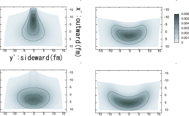
Figure 1: Contour plots of the effective source distribution $\tilde{\rho}_{\rm eff.}({\bm{x}}^{\prime},{\bm{k}})$ defined by (31) at $k=100$MeV/c. Left (right) columns correspond to results with repulsive (attractive) potential. Lower panels include effect of absorption. Vertical (horizontal) coordinate denotes the shifted outward (sideward) location of the emission points whose plot range is distorted by the non-linear coordinate transformation.

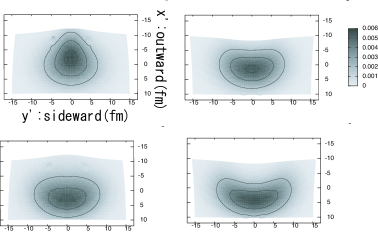
Figure 2: Contour plots of the effective source distribution at $k=150$MeV/c. Each panel corresponds to the same choice of the potential at the same location in Fig.1

We show in Fig. 1 contour plots of the effective source image at $k=100$MeV/c. The upper two panels give the results with no absorption (${\cal V}_{i}=0$) while the lower panels are computed with ${\cal V}_{i}=0.1$ MeV. The vertical and horizontal coordinates gives the apparent location of the emission points in the outward direction (direction of ${\bm{k}}$) and the sideward direction (direction perpendicular to ${\bm{k}}$) respectively. We first compare the case for repulsive interaction ${\cal V}_{1}=10$ MeV with no absorption (upper left panel) and the attractive interaction with no absorption (upper right panel). We found that the real part of potential affects on the extension of source in both outward and sideward directions. The repulsive interaction leads to elongation of the effective source image in the outward direction, while the attraction tends to shrink the source in this direction. On the other hand, the repulsive force leads to shrinking sideward source extension, while the attractive force gives the sideward extension stretched. These effects are seen as a geometrical effect of either stretching or compressing the scale of each coordinate. The distortion of the original image is weakened as the momenta of the two particles increases as seen in Fig. 2 at $k=150$MeV/c.

Our results qualitatively agree with the results of two other groups[15, 16]. Pratt and Cramer et al. suggested that this change of the apparent source size in the sideward direction may be interpreted as due to the refraction or the lensing effect in geometrical optics. In our analyses, however, the apparent shift of the emission point is caused by the ${\bm{k}}$ dependence of the phase shift $\delta W({\bm{x}},{\bm{k}})$, through Eq. (26): the apparent shift of the emission point $\delta{\bm{x}}=-\nabla_{\bm{k}}\delta W({\bm{x}},{\bm{k}})$ arises due to the difference of the action of the potential for particles traversing along two adjacent trajectories starting at the same point ${\bm{x}}$ ending up with different final momenta.

To make this issue more quantitative, we examine the phase shift using Glauber-type approximation which assumes the straight-line trajectories in the interaction regions so that the phase shift is given by the simple formula which may be written for $V<<{\bm{k}}^{2}/2m$,

$$\delta W_{\rm Glauber}(\bm{x},{\bm{k}}) \simeq -\frac{m}{|{\bm{k}}|}\int_{u(0)}^{u(T)}V(\sqrt{u^{2}+b^{2}})du$$ (31)

where $b=\sqrt{{\bm{x}}^{2}-({\bm{x}}\cdot{\bm{k}})^{2}/{\bm{k}}^{2}}$ is the ”impact parameter” of the trajectory, and $u(t)={\bm{x}}(t)\cdot{\bm{k}}/|{\bm{k}}|$ is the position of the particle along the trajectory at time $t$. This phase shift depends on $\theta_{\bm{k}}$ since $b$ is related to ${\bm{k}}$ by $b=\sqrt{{\bm{x}}(T)^{2}-({\bm{x}}(T)\cdot{\bm{k}})^{2}/{\bm{k}}^{2}}$ at large time $T$. The change of the HBT image calculated by this formula is shown in Fig.3 for the same cases as in Fig.1. It is seen that the ”Glauber approximation” qualitatively reproduces the same results. This implies that the deflection of the classical trajectory in the source region is not essential for the distortion of the HBT images; rather, the change of the relative momentum of two particles via the difference of their phase shifts is the origin of the distortion of the source image.

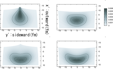
Figure 3: The effective source distributions at $k=100$MeV/c in the Glauber approximation computed with the same potentials as in Fig.1

The inclusion of the absorption, however, diminishes all these interesting effects of the mean field interaction, by effectively cutting off the contributions from deep interior of the source as well as the other side of the source. The result is somewhat similar to the effect caused by the attractive interaction, namely the source image is effectively stretched in the sideward direction.

Although we still need to make improvements in our calculations (relativistic treatment, time-dependent source structure[17, 18], more realistic pion optical potential, etc.) before confronting the experimental data, these mean field effects may play some role in reducing the discrepancy between the data and hydrodynamic simulations at small values of $k$.

In conclusion, we have studied the effect of the final state interaction in the meson clouds on the HBT interferometry in heavy-ion collisions and have shown that the final state interaction causes a significant distortion of the source images at small $k$ through the change of the phase shift in the single particle amplitude and the absorption effect. More detail account of this work will be reported elsewhere.

References

• [1] R. Hanbury Brown and R. Q. Twiss, Nature 177, 27 (1956)
• [2] R. J. Glauber, Phys. Rev. Letts. 10, 84 (1963)
• [3] F. B. Yano and S. Koonin, Phys. Letts. B78, 556 (1978)
• [4] M. Gyulassy, S. K. Kauffmann, L. W. Wilson, Phys. Rev. C20, 2267 (1979)
• [5] G. Baym, Acta. Phys. Polon. B 29 1839 (1998)
• [6] C. Adler et al. (STAR Collaboration), Phys. Rev. Lett. 87 082301 (2001)
• [7] K. Adcox et al. (PHENIX Collaboration), Phys. Rev. Lett. 88 192302 (2002)
• [8] T. Hirano, K. Tsuda, Phys. Rev. C 66 054905 (2002)
• [9] M. A. Lisa, S. Pratt, R. Soltz and U. Wiedemann, Ann. Rev. Nucl. Part. Sci. 55 357 (2005)
• [10] S. Adler et al. (PHENIX collaboration), Phys. Rev. Lett. 98, 132301 (2007); S. Afanasiev et al. (PHENIX collaboration), Phys. Rev. Lett. 100, 232301 (2008)
• [11] P. Danielewicz, S. Pratt, Phys. Rev. C 75 034907 (2007)
• [12] M. C. Chu, S. Gardner, T. Matsui, R. Seki, Phys. Rev. C 50 3079 (1994)
• [13] J. D. Bjorken, Phys. Rev. D27, 865 (1983)
• [14] Similar analysis has been done for the long range Coulomb interaction in G. Baym, P. Braun-Munzinger, Nucl. Phys. A 610 286c (1996)
• [15] G. Cramer, G. Miller, J. Wu and Jin-Hee Yoon, Phys. Rev. Lett. 94 102302 (2005)
• [16] S. Pratt, Phys. Rev. C 73 024901 (2006)
• [17] G. Bertsch, G. Brown, Phys. Rev. C 40 1830 (1989)
• [18] D. Rischke, M. Gyulassy, Nucl. Phys. A 608 479 (1996)