Identification and Query of Activated Gene Pathways in Disease Progression

Abstract

Disease occurs due to aberrant expression of genes and modulation of the biological pathways along which they lie. Inference of activated gene pathways, using gene expression data during disease progression, is an important problem. In this work, we have developed a generalizable framework for the identification of interacting pathways while incorporating biological realism, using functional data analysis and manifold embedding techniques. Additionally, we have also developed a new method to query for the differential co-ordinated activity of any desired pathway during disease progression. The methods developed in this work can be generalized to any conditions of interest.

1 INTRODUCTION

A gene is a segment of the genome (DNA) that codes for protein. Proteins are the biological catalysts of function and mediate the kinetics and timing of any biological process. The body is composed of several tissues and each tissue has its own individual lineage of cells. The set of proteins that are active in each cell are different depending on cell context and the underlying function of the cell. Since proteins are encoded by the gene(s), it is believed that biological processes are orchestrated by a precise spatio-temporal expression of genes. Gene activities in the cell are organized along pathways, which might either have signaling activity or regulatory role in determining cell behavior. Thus even though there is a heterogeneous population of cells in the body, each set of cells has a precise time and location of gene/pathway expression corresponding to required protein activity.

Systemic disease can occur due to the mis-expression of genes in various tissues [as an example, the Gata3 gene is mutated in HDR (hypoparathyroidism, deafness, renal dysplasia)]. A lot of studies have studied the link between the genome and the phenome - i.e. between gene expression and physical characteristic. Disease (and its symptoms) is a physical characteristic which arises from mis-expression of the underlying genome. Also, very rarely is disease due to the aberrant expression of a single gene - they mostly arise due to mis-expression of several genes at once (i.e. gene sets). Identifying these set of aberrant genes (or pathways) is an important problem because of the immense therapeutic potential. There is an ongoing effort to find inhibitors that can target disease-implicated pathways. For example, two well-known drugs Gleevec and Tarceva target receptor tyrosine kinase signaling pathways that have a reported role in cancer [RTK_book].

In this work, we develop methods to identify pathways (Part $I$) that have a role in disease progression. Specifically, we ask which pathways are potentially modulated during onset and evolution of immune response to infection. Additionally, we present a framework (Part $II$) that can query the differential activity of ‘any’ pathway between normal and diseased states, thereby allowing for the principled selection of pathway inhibitors to modulate and control disease. Using time series expression profiles of gene expression, we use functional data analysis (FDA) to process, analyze and cluster the data into possible pathway components. In addition, we use a manifold embedding technique to improve on these results and extend this for generalized pathway querying.

2 OUTLINE

This paper is organized as follows. To interpret pathway activity during immune response, section 3 deals with the examination of the gene expression data during pathogen infection, and its representation in terms of B-spline basis functions. Section 4 uses principal component analysis on the functional data (fPCA) to discover modes of variation in the data. This is followed by clustering genes in fPCA space to find genes whose interaction is putatively associated with infection. We find that the results are not directly relevant biologically and hence, section 8 develops methods to improve the context of the clustering results to obtain more meaningful results. This new framework enables the solution of another hitherto unexamined problem - querying any arbitrary pathway for co-ordinated differential activity between case and condition (section 9). As an example, we examine the activity of the Toll-like receptor (TLR) pathway for the pathogen infection data set, and demonstrate the general utility of this approach in such problems. Section 11 concludes the paper.

3 DATA EXTRACTION AND PRE-PROCESSING

One of the most common processes involving gene-pathway modulation is the systemic response of the immune system to an invading pathogen. With the advent of whole genome microarrays that can assay the activity of genes over a time course, expression profiling of genes during the innate and adaptive immune response has been actively pursued for the identification of genes that can be used for diagnostic or therapeutic purposes. For this study, in order to find pathways implicated in the immune response to pathogen infection, we use functional expression data gathered by the Young group [Young_data]. This data profiles the various gene activation programs initiated in macrophage cells on exposure to various pathogens such as tuberculosis, e.coli and staphylococcus aureus. There is also a set of control treatments in which latex beads coated without bacteria are presented to the macrophage cell population. In this study, we consider the differential pathway activity between tuberculosis and control conditions. The methods developed in our approach are however, more general and can be applied for any number of interesting conditions.

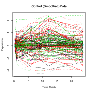
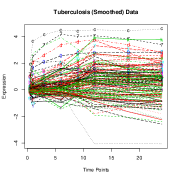
The dataset contains expression values at $8$ time points for $168$ unique macrophage genes. These correspond to gene expression profiling $0.5,1,3,6,12,16,18,24$ hours after exposure with the pathogen (or control). Since macrophages exhibit an early innate as well as late adaptive immune response, it is interesting to examine which genes are expressed in a certain phase.

To use the functional data approach on the raw data, we start by representing the functional data via B-spline basis functions. This choice of basis functions is primarily governed by the lack of inherent periodicity in immune response over the first $24$ hours, as well as the possibility of local structure in the time series that are are relevant to analysis. Using the “FDA” package in R, we create B-spline basis functions ($B_{k}(t_{j})$) of order $3$ and $J=46$ internal knots over the interval $[0.5,24]$. Under this representation, we have,

$x_{i}(t_{j})=\sum_{k=1}^{K}c_{k}B_{k}(t_{j})$ for $i=1,2,\ldots,n$ with $n=168$.

Furthermore, a smoothing operation is implemented on the data (using generalized cross-validation), with $\lambda=0.001$. The plots of the functional data after smoothing are displayed in Fig. 1(a) and Fig. 1(b) respectively.

4 FUNCTIONAL PRINCIPAL COMPONENT ANALYSIS (fPCA)

Functional PCA (fPCA) aims to find a solution to the eigenvalue problem [ramsay_1997, ramsay_2002] : $C\mathbf{\phi}\textbf{b}=\lambda\textbf{b}$, where $C=[\sum_{i=1}^{n}c_{i,k}c_{i,l}/n]$, $\phi=[\langle B_{k},B_{m}\rangle]$ and $\mathbf{b}=(b_{1},b_{2},\ldots,b_{k})$. The $j^{th}$ principal component eigenvector $\mathbf{b}_{j}$ of $C\phi$ leads to an estimate $\epsilon_{j}=[B_{1},B_{2},\ldots,B_{K}]^{T}\mathbf{b}_{j}$ of the eigenfunction. With this, the $j^{th}$ principal component score is given by $\alpha_{i,j}=\langle x_{i},\epsilon_{j}\rangle$. The set of scores ($[\alpha_{i,1},\alpha_{i,2},\ldots,\alpha_{i,p}]\in\mathbb{R}^{p};i=1,2,\ldots,168$) can then be used for clustering [Morris_fda].

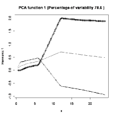
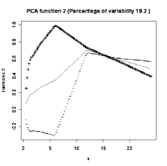
To understand the modes underlying disease onset and its response by the immune system, a fPCA analysis of the data was done. The first and second principal components of the tuberculosis functional data are displayed in Fig. 2 (a) and (b) respectively. These harmonics correspond to the components after varimax rotation to aid interpretability (ramsay_1997,ramsay_2002). The harmonic plots indicate two distinct behaviors and are indicative of typical immune response.

(a) Smoothed Control time-series Data.

(b) Smoothed Tuberculosis time-series Data.

Figure 1: Smoothed functional data for immune response under tuberculosis and control. The x-axis denotes the time points in hours.

Some interesting insights emerge from the plots of Fig. 2. The first harmonic corresponds (roughly) to the ‘late’ variation in gene expression (Fig. 2, accounting for $\sim 78\%$ variation) whereas the second principal component corresponds to the ‘early’ variation (Fig. 2, accounting for $\sim 20\%$ variation). This is extremely meaningful because the principal components correspond to a drastic change in adaptive immune response and is strongly associated with biological response to pathogen infection. This is also known from biological literature [Young_data, Huang_Hacohen].

The scores of the functional tuberculosis gene data along these first two principal components is shown in Fig. 3(a).

5 MODEL-BASED CLUSTERING

Having found scores of each of the genes in fPCA space, our goal is to now group (cluster) genes with similar temporal profiles. In this section, we derive the parameter update equations for a Mixture of Gaussian clustering paradigm [MClust_TR, GMM_PAMI].

Figure 2: First and Second Functional Principal Components for Tuberculosis data. X-axis corresponds to assay time points, as in the previous plots. We note that the solid line in each case corresponds to the mean function, the $(+)$ line corresponds to the mean function added to a multiple of the harmonic and the $(-)$ line corresponds to a subtraction of the harmonic function.

We consider the group of gene expression profiles $\mathscr{G}=\{\boldsymbol{g^{(1)}},\boldsymbol{g^{(2)}},\ldots,\boldsymbol{g^{(n)}}\}$, all of which share a common dynamic. Consider gene profile $i$, $\boldsymbol{g^{(i)}}=[\alpha_{i,1},\alpha_{i,2},\ldots,\alpha_{i,J}]$, a $J$-dimensional random vector (here $J=2$) which follows a $k$-component finite mixture distribution described by:

$$p(\textbf{g}|\boldsymbol{\theta}) =\sum_{m=1}^{k}\alpha_{m}p(\textbf{g}|\boldsymbol{\phi_{m}})$$ (1)

where $\alpha_{1},\ldots,\alpha_{k}$ are the mixing probabilities, each $\phi_{m}$ is the set of parameters defining the $m^{th}$ component, and $\boldsymbol{\theta}\equiv\{\phi_{1},\ldots,\phi_{k},\alpha_{1},\ldots,\alpha_{k}\}$ is the set of complete parameters needed to specify the mixture. We have,

$$\alpha_{m}\geq 0,m=1,\ldots,k,\quad and\quad\sum_{m=1}^{k}\alpha_{m}=1$$ (2)

(a) Scores of functional data along functional principal components, PC1 and PC2

(b) BIC plot during model-based clustering

Figure 3: Embedding of data onto fPCA space and BIC plot to find optimal cluster number.

For a set of $n$ independently and identically distributed samples,

$$\mathscr{G} =\{\boldsymbol{g^{(1)}},\boldsymbol{g^{(2)}},\ldots,\boldsymbol{g^{(n)}}\},$$ (3)

the log-likelihood of a $k$-component mixture is given by:

$$\log p(\mathscr{G}|\boldsymbol{\theta}) =\log\prod_{i=1}^{n}p(\boldsymbol{g^{(i)}}|\boldsymbol{\theta})$$ (4)

$$\quad=\sum_{i=1}^{n}log\sum_{m=1}^{k}\alpha_{m}p(\boldsymbol{g^{(i)}}|\phi_{m})$$ (5)

• Treat the labels, $\mathscr{Z}=\{\boldsymbol{z^{(1)}},\ldots,\boldsymbol{z^{(n)}}\}$, associated with the $n$ samples - as missing data. Each label is a binary vector $\boldsymbol{z^{(i)}}=[z_{1}^{(i)},\ldots,z_{k}^{(i)}]$, where $z_{m}^{(i)}=1$ and $z_{p}^{(i)}=0$, for $p\neq m$ indicates that sample $\boldsymbol{g^{(i)}}$ was produced by the $m^{th}$ component.

In this setting, the Expectation Maximization algorithm can be used to derive the cluster parameter $(\boldsymbol{\theta})$ update equations.

In the E step of the EM algorithm, the function $Q(\boldsymbol{\theta},\boldsymbol{\hat{\theta}}(t))\equiv E[\textrm{log}p(\mathscr{G,Z}|\boldsymbol{\theta})|\mathscr{G},\hat{\boldsymbol{\theta}}(t)],$is computed. This yields,

$$w_{m}^{(i)}\equiv E[z_{m}^{(i)}|\mathscr{G},\hat{\theta}_{t}] =\frac{\hat{\alpha}_{m}(t)p(\boldsymbol{g^{(i)}}|\boldsymbol{\hat{\theta}_{m}}(t))}{\sum_{j=1}^{k}\hat{\alpha}_{j}(t)p(\boldsymbol{g^{(i)}}|\boldsymbol{\hat{\theta}_{j}}(t))}$$ (6)

where $w_{m}^{(i)}$ is the posterior probability of the event $z_{m}^{(i)}=1$, on observing $g_{m}^{(i)}$.

The estimate of the number of components ($$k$$) is chosen using a bayesian information criterion (BIC) criterion [MClust_TR, GMM_PAMI]. The BIC criterion borrows from information theory and serves to select models of lowest complexity to explain the data. As can be seen below, this complexity has two components - the first encodes the observed data as a function of the model and the second encodes the model itself. Hence, the BIC criterion in our setup becomes, :

$$\hat{k}_{BIC} =\textrm{argmax}_{k}\{2\textrm{log}p(\mathscr{G}|\boldsymbol{\hat{\theta}}(k))-\frac{k(N_{p}+1)}{2}\textrm{log}n\},$$ (8)

$N_{p}$ is number of parameters per component in the $k$ component mixture, given the number of clusters $k_{min}\leq k\leq k_{max}$. $n$ is the total number of observations.

In the M step: For $$m=0,1,\ldots,k, \hat{\theta}_{m}(t+1)=\arg\max_{\phi_{m}}Q(\boldsymbol{\theta},\hat{\boldsymbol{\theta}}(t)) m:\hat{\alpha}_{m}(t+1)>0 \hat{\phi} \boldsymbol{\hat{\theta}} p(\boldsymbol{g^{(i)}}|\boldsymbol{\phi_{m})} p(\textbf{g}^{(i)}|\phi_{m}) \mathscr{N}(\boldsymbol{\mu}_{m},\boldsymbol{\Sigma}_{m}) \phi=(\boldsymbol{\mu},\boldsymbol{\Sigma})$$ , for , the elements ’s of the parameter vector estimate are typically not closed form and depend on the specific parametrization of the densities in in the mixture, i.e. . If belongs to the Gaussian density class, we have, and EM updates yield [12],

$$\hat{\alpha}_{m}(t+1)=\frac{\sum_{i=1}^{n}w_{m}^{(i)}}{n},$$ (10)

$$\boldsymbol{\mu}_{m}(t+1)=\frac{\sum_{i=1}^{n}w_{m}^{(i)}\textbf{g}^{(i)}}{\sum_{i=1}^{n}w_{m}^{(i)}},$$ (11)

$$\boldsymbol{\Sigma}_{m}(t+1)=\frac{\sum_{i=1}^{n}w_{m}^{(i)}(\textbf{g}^{(i)}-\mu_{m}(t+1))(\textbf{g}^{(i)}-\mu_{m}(t+1))^{T}}{\sum_{i=1}^{n}w_{m}^{(i)}}$$ (12)

The equations 5. $6,8,9,10$ are the parameter update equations for each of the $m=1,\ldots k$ cluster components.

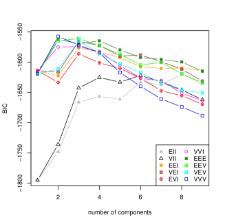
The R package ‘MClust’ can be used to do model based clustering on the genes (represented as fPCA scores). The method enables the selection of the optimal number of clusters via maximizing the bayesian information criterion (BIC). It outputs a plot that displays the BIC for each cluster assignment, where the clusters can have three independent degrees of freedom (shape, volume and orientation). The optimal cluster assignment is chosen from all possibilities of shape, volume, orientation and BIC [MClust_TR].

6 fPCA CLUSTERING RESULTS

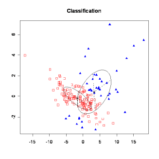
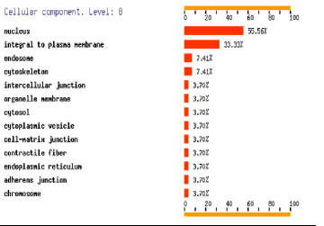
Based on the Bayesian Information criterion (BIC), we select two clusters (Fig. 4(a)) with variable shape, volume and orientation (VVV). Additionally, to ascertain the purity of clustering, we examine if co-clustered genes are in the same cellular location. This is done using the FATIGO$+$ tool at http://babelomics.bioinfo.cipf.es/fatigoplus/. The results of this analysis is in Fig. 4(b). The results indicate that only about 50% of the co-clustered genes are co-located (in the nucleus). This casts serious doubts on the analysis methods of previous papers that use clustering in PCA/fPCA space as a method to discover novel pathway components. Biologically, the cellular proximity of two genes is essential for their interaction along a pathway. Thus, unless cellular proximity can be explicitly incorporated into this framework, such clustering can potentially fail in the discovery of true pathway components [go_clust2, go_clust].

(a) BIC based model clustering.

(b) GO purity of Clusters from fPCA.

Figure 4: BIC based clustering for fPCA embedded data and GO cluster purity.

7 COMMENTS

To recapitulate, there is a need to find molecular signatures that predict grade of disease/ therapeutic potential. The traditional approach to find dysregulated pathways is based on clustering genes based on expression profiles (for the corresponding disease) – in fPCA space. This uses the hypothesis that co-clustered (co-expressed) genes are ‘possibly’ part of the same pathway – since genes with similar expression profiles all belong to same pathway, i.e. their relationship is so tight that they will behave in the same coordinated manner. A lot of literature using this hypothesis is available.

However, this approach is questionable because in any biological process, several pathways are involved, and there are cross-interactions (cross-talk) among pathways. Clusters can thus consist of putatively interacting pathways, not just one pathway. Because different conditions/diseases are due to different aberrant pathways, clusters can have different sets of genes and thus several ‘true’ pathways. This leads to incorrect inference of the biology, because every study can find a‘new’ pathway based on which condition they study. In reality, there are only a few standard pathways – however their interactions are different in different diseases/conditions.

Thus, we would need to incorporate some other prior knowledge to aid the clustering approach in achieving biological realism. One such way would be to use location information in conjunction with expression and cluster genes in that combined space – this follows from fact that if genes have to have coordinated pathway activity, they should be nearby in cellular location.

8 Part I: BUILDING REALISM WHILE CLUSTERING

As suggested in the previous sections, it would be useful to have a “space” which respects physical cellular proximities in addition to expression similarities. This can be enabled by considering a set of annotations that describe the “cellular location” information for each of the genes (in the macrophage activation program). One set of annotations that is well researched by the bioinformatics community is the Gene Ontology (GO) descriptors (http://www.geneontology.org/). This is a controlled hierarchical vocabulary that annotates genes in various organisms by cellular component (CC), molecular function (MF) and biological process (BP), based on literature reports.

The next section examines the generation of a “semantic similarity matrix” between genes based on their GO (CC) descriptors, to quantify the cellular proximity among them. Just like lexical word ontologies for spoken languages (e.g. WordNet at http://wordnet.princeton.edu/), this structure imposes a tree structure on the various GO terms, thereby expressing the similarity between any two terms in the ontology as a function of their parents in the ontology tree.

The next step involves the use of manifold embedding techniques that can integrate such GO similarity along with expression-level similarity to construct an embedding of the genes as points in some space. One such technique is Laplacian Eigenmaps [Laplacian], also profiled in Section: 8.2 that approximate both these relationships (semantic and expression similarities). This is a generalization of the principal component approach in that the distance measures on such manifolds are not necessarily euclidian. After embedding the genes onto this manifold, we will then re-examine the model based clustering approach and assess the GO purity (as in section: 6) of the obtained clusters.

We remind the reader that the main goal here is to embed genes based on their expression profiles, but additionally weighted based on their cellular proximity – this would be more biologically relevant for the discovery of true pathway activity. We believe that such an approach is consistent with the rationale of using integrative genomics or principled heterogeneous data integration for stronger hypothesis generation [data_integration].

8.1 GO Semantic Similarity

To quantify the notion of similarity of terms along an ontology, we appeal to a vast amount of literature that addresses such questions [Semantic_Similarity]. The semantic similarity of any two GO terms along the ontology hierarchy is based on the number of shared parents and the information content of the individual GO terms (measures: Jiang Conrath, Resnik etc.). Based on the literature, we use the Jiang-Conrath similarity measure, given by,

$W_{i,j}=sim(c_{i},c_{j})=\frac{1}{jc_{dist}(c_{i},c_{j})}$, with $jc_{dist}(c_{i},c_{j})=2log(p(lso(c_{i},c_{j})))-[log(p(c_{i}))+log(p(c_{j}))]$

where $c_{i}$ and $c_{j}$ are two terms (nodes) along the GO ontology tree ($i,j\in\{1,2,\ldots,168\}$). $lso(c_{i},c_{j})$ refers to the the information content of the last common parent of these two nodes. The information content is computed based on the probabilities of observing the individual nodes and their last common ancestor in an overall corpus.

For the $168$ genes profiled in this study, we use the R package “GOSim” to obtain the semantic similarity matrix (size $168\times 168$) based on GO location annotation. This similarity matrix is used to obtain the weight matrix $W$ during the Laplacian Eigenmap embedding procedure [Laplacian] below.

8.2 LLE (Laplacian Eigenmaps)

• Build the $K\times K$, $(K=168)$ dimensional weight matrix $W$ from the Gene Ontology (“Cellular Component”) terms of the genes in the dataset. This distance is the “normalized” semantic similarity alluded to above (section 8.1).

• Assign weight $W_{i,j}$, from (1) for each gene pair $(i,j)$, for each of the ${K\choose 2}$ gene pairs. Note: The higher this weight, the closer the genes are.

• Find $n$ nearest neighbors using the euclidian distance in principal component space. The scores of the functional data along the first two principal components can be interpreted as co-ordinates in a euclidian space.

• Form the Graph Laplacian:

  $$L_{i,j}=\left\{\begin{array}[]{ll}d_{i}=\sum_{k}W_{i,k}&\mbox{if $i=j$};\\ -W_{i,j}&\mbox{if $i\text{ is connected to }j$};\\ 0&\mbox{otherwise}.\end{array}\right.$$

  
  

• Solve: $min_{y}y^{T}Ly=\frac{1}{2}\sum_{i,j}(y_{i}-y_{j})^{2}W_{i,j}\quad(2)$,
  subject to:

  • $y^{T}Dy=1$, and
    

  • $y^{T}D\textbf{1}=0$,

  where $D_{i,i}=\sum_{j}W_{j,i}$, a diagonal weight matrix.

• Embed the co-ordinates to a lower dimensional manifold, using the solution (the Laplacian Eigenmap) obtained from the minimization above.
  

  • The solution to (2) is given by the d generalized eigenvectors associated with the d smallest generalized eigenvalues solving $L\textbf{y}=\lambda D\textbf{y}$ (neglecting the zero eigenvalue and its eigenvector).

  • If $\textbf{y}=[y_{1},\ldots,y_{d}]$ is the collection of these eigenvectors, then the embedding is given by :
    $y_{i}=(y_{i1},\ldots,y_{id})^{T}$, i.e., the $d$ dimensional representation of the $i^{th}$ data point (gene).

• In our representation, we take dimensionality, $d$ = 2 and number of neighbors, $n$ = 5. The final embedding of the functional data based on expression and location modalities is shown in Fig. 5(a).

(a) Eigenmap embedded data.

(b) BIC plot for Eigenmap based clustering.

Figure 5: Eigenmap based embedding and BIC plot.

8.3 Results with Laplacian Eigenmaps

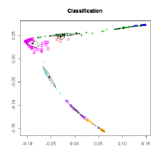
After transforming the original scores (from fPCA) based on the GO semantic similarity matrix $W$, the $2D$ representation of the gene data is shown in Fig. 5(a). Based on this new embedding, which leads to a very different visualization of the data compared to Fig. 3(a), we can once again use model based clustering in the new space.

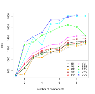
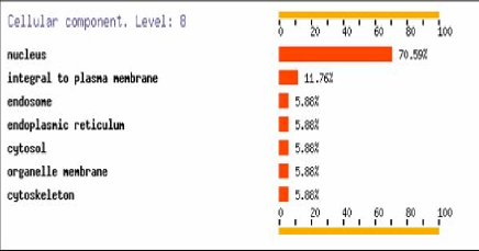
Based on this, the BIC plot for the Eigenmap embedded data is shown in Fig. 5(b). The highest BIC corresponds to $8$ clusters (Fig. 6(a)) with variable shape, volume and orientation (VVV). An examination of the GO (“cellular component” annotation) is shown in Fig. 6(b). This indicates that the GO enrichment of genes that are close by (like in nucleus) is much higher ($\sim 70\%$ compared to $55\%$ before). Furthermore, interrogation of a cluster in the new assignment (after Eigenmap embedding) clearly identifies known components of the cytokine pathway [Huang_Hacohen] (several interleukin members). This shows that an embedding, that respects location as well as expression simultaneously, identifies closely interacting pathway components via clustering. This aids in the development of biologically relevant hypotheses.

(a) Clustering on Eigenmap embedded data.

(b) GO purity of Eigenmap based clustering.

Figure 6: BIC based clustering for Eigenmap embedded data and GO purity.

9 Part II: QUERYING PATHWAY ACTIVITY

The first part of this work presents a principled framework to embed gene relationships based on expression and cellular location. This framework can now be extended to understand the co-ordinated activity of genes constituting a pathway. We note that this question has not hitherto been asked in this context previously. Previous methods have only looked at identifying pathway genes based on expression similarities. In the light of the previous analysis suggesting that plain clustering in expression space without regard to physical proximity might not be biologically relevant, this framework enables the integration of multiple modalities to obtain much more relevant results. Embedding the data using a principled approach enables the formulation of more complex queries such as coordinated pathway activity.

The key question that can now be addressed under the above framework is: How strongly is pathway ‘X’ dysregulated between normal cells and diseased (tuberculosis infected) cells. A pathway is a set of interacting genes. More generally, one can query for the co-ordinated activity of any subset of interesting genes (generalizing the approach of [GSEA, GSA].

9.1 Querying Pathway Activity

In order to query a pathway’s activity, we can first obtain the known components (genes) of the pathway using resources such as the KEGG (http://www.genome.ad.jp/kegg/pathway.html) or BioCarta (http://cgap.nci.nih.gov/Pathways/BioCarta_Pathways) pathway repositories.

For any query pathway P (consisting of $k$ genes),we can find the co-ordinates of this subset on the manifold embedding obtained above. Let $C_{p}$ be the inter-point distance matrix ($k\times k$) of the $k$-gene pathway in the eigenmap for the control condition. Let $T_{p}$ be the inter-point distance matrix of the k-gene pathway under the perturbation (tuberculosis infection).

In this setting, the question of querying pathway activity translates to the following question: How are the gene-gene associations among these $k$-components of the pathway “different” between control ($C_{p}$) and case ($T_{p}$).

This is addressed in the following section. The idea is to find a metric of similarity (or distance) between the distance matrices ($C_{p}$ and $T_{p}$). The Mantel correlation test has been used in ecological studies as a similarity metric. The other is a hitherto unused metric, termed the logDet divergence, that has been used in other applications (to quantify the distributional divergence between two probability distributions).

9.2 Quantifying difference in association matrices

Based on the above, the Mantel’s test is used in ecological analysis (R package “vegan”) to compare two (or more) spatial proximity matrices. In our context, we are interested to ask if the gene set that is close in one space (control) is also close in the other space (tuberculosis).

The Mantel correlation coefficient between two ($k\times k$) matrices $X$ and $Y$ - $`r^{\prime}$ is given by [Mantel_test ]:

$r=\frac{1}{(n-1)}\sum_{i<j}\frac{x_{ij}-\bar{x}}{s_{x}}.\frac{y_{ij}-\bar{y}}{s_{y}}$

Here, $X=C_{p}$ and $Y=T_{p}$. $s_{x}$ and $s_{y}$ are the standard deviations from the entries of the matrices $X$ and $Y$, respectively (for normalization); $n=\frac{k(k-1)}{2}$. The higher the value of $`r^{\prime}$, the more similar the two distance matrices are.

Finally, we can estimate a significance of $r(T_{p},C_{p})$ via bootstrapping. This would involve the following steps:

• Repeat the following procedure B$(=1000)$ times (with index $b=1,\ldots,B$):

  • Generate resampled (with replacement) versions of the matrices $C_{p}$, $T_{p}$, denoted by $C_{p}^{b}$, $T_{p}^{b}$ respectively.

  • Compute the statistic $\theta^{b}$ = $r(T_{p}^{b},C_{p}^{b})$.

• Construct an empirical CDF (cumulative distribution function) from these bootstrapped sample statistics, as $F_{\Theta}(\theta)=P(\Theta\leq\theta)=\frac{1}{B}\sum_{b=1}^{B}I_{x\geq 0}(x=\theta-\theta^{b})$, where $I$ is an indicator random variable on its argument $x$.

• Compute the true detection statistic (on the original time series) $\theta_{0}=r(T_{p},C_{p})$ and its corresponding $p$-value ($p_{0}=1-F_{\Theta}(\theta_{0}))$ under the empirical null distribution $F_{\Theta}(\theta)$.

• If $F_{\Theta}(\theta_{0})\geq(1-\alpha)$, then we have that the true mantel correlation value is significant at level $\alpha$, leading to rejection of null-hypothesis (no association).

9.3 logDet divergence

The logDet divergence has recently received a lot of interest in the machine learning community, mainly with regard to metric learning problems [metric_learning]. To see an example of how they arise, consider the the Kullback-Liebler (KL) divergence between two multivariate Gaussian densities $p(x;C_{p})$ and $p(x;T_{p})$. This is given by:
$KL(p(x;C_{p})||p(x;T_{p}))=\frac{1}{2}D_{ld}(C_{p},T_{p})$, where,

$D_{ld}$ is the logDet divergence between two positive definite matrices $C_{p}$ and $T_{p}$ defined by:

$D_{ld}(C_{p},T_{p})=tr(C_{p}T_{p}^{-1})-logdet(C_{p}T_{p}^{-1})k$  ($k$ is the rank of the matrices $C_{p}$ and $T_{p}$)

We note that the distance matrices $C_{p}$ and $T_{p}$ are positive semi-definite, but can be made positive definite via the addition of a constant term to its non-diagonal elements [Cailiez_method] (Cailiez method). Before using the logDet criterion, the distance matrices need to be converted into correlation matrices (this can be done via a scaled exponential transformation [Laplacian]. Additionally, since the KL divergence is not intrinsically symmetric, the symmetrized version, $LD_{dist}(T_{p},C_{p})=\frac{1}{2}D_{ld}(C_{p},T_{p})+\frac{1}{2}D_{ld}(T_{p},C_{p})$ can be used instead. The higher the value of this symmetrized distance, the higher the dissimilarity between $C_{p}$ and $T_{p}$.

Finally, we can estimate a significance of $LD_{dist}(T_{p},C_{p})$ via bootstrapping. This would involve the following steps:

• Repeat the following procedure B$(=1000)$ times (with index $b=1,\ldots,B$):

  1. Generate resampled (with replacement) versions of the matrices $C_{p}$, $T_{p}$, denoted by $C_{p}^{b}$, $T_{p}^{b}$ respectively.

  2. Compute the statistic $\theta^{b}$ = $LD_{dist}(T_{p}^{b},C_{p}^{b})$.

• Construct an empirical CDF (cumulative distribution function) from these bootstrapped sample statistics, as $F_{\Theta}(\theta)=P(\Theta\leq\theta)=\frac{1}{B}\sum_{b=1}^{B}I_{x\geq 0}(x=\theta-\theta^{b})$, where $I$ is an indicator random variable on its argument $x$.

• Compute the true detection statistic (on the original time series) $\theta_{0}=LD_{dist}(T_{p},C_{p})$ and its corresponding $p$-value ($p_{0}=1-F_{\Theta}(\theta_{0}))$ under the empirical null distribution $F_{\Theta}(\theta)$.

• If $F_{\Theta}(\theta_{0})\geq(1-\alpha)$, then we have that the true logDet value is significant at level $\alpha$, leading to rejection of null-hypothesis (complete association).

10 CASE STUDY:TLR PATHWAY

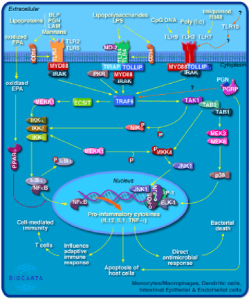
As an example of querying pathway activity, we analyse the toll-like receptor (TLR) pathway. Members of the toll-like receptor (TLR) gene family convey signals stimulated by various pathogenic factors, activating signal transduction pathways that result in transcriptional regulation and stimulate innate immune function (Fig. 7(a)). Hence it is one of the earliest and most strongly activated pathways during immune response.

(a) TLR pathway (©Biocarta).

(b) Null Histogram of the logDet divergence for the TLR pathway. True value=0.5513. Is Activated Early in Immune Response

Figure 7: The TLR pathway and its Divergence between normal and case conditions.

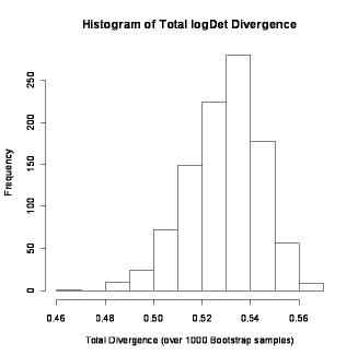
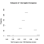
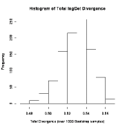
For this pathway, we get the subset of genes that are common between the Biocarta TLR catalog and the set of $168$ genes. For those $7$ genes, we can find the inter-point distance matrices along the normal and infection cases. The value (also referred to as the true value) of the mantel correlation and logDet divergence (between the normal and control states) is $0.0447$ and $0.5513$ respectively, suggesting that the association between these two distance matrices is fairly low. Additionally, these correlation and divergence values are significant at the $0.05$ level with respect to the null distribution (Fig. 7(b)). Hence, these two measures are useful at picking up a truly activated pathway between these two conditions. In the same way, one can obtain these two measures for any chosen pathway of interest, yielding results that are concordant with literature [Huang_Hacohen]. This is shown in Table $I$.

(a) Null Histogram for the TLR pathway components. True value=0.5513. Is Activated Early in IR.

(b) Null Histogram for the Mapk pathway components. True-value: 0.018. Not activated early.

Figure 8: Bootstrapping results from Toll-like Receptor (TLR) and Mapk pathways.

Mantel and logDet values of some interesting pathways. Pathway Name Mantel test (value and significance) logDet divergence (value and significance) Apoptosis 0.5961(0.038) 0.149(0.025) Toll-like receptor (TLR) 0.047(0.0255) 0.5513(0.032) Mapk 0.3373(0.142) 0.018(0.010) T/B-cell 0.271(0.071) 0.1523(0.006)

11 CONCLUSIONS

In Part $I$ of this work, we demonstrated a generalizable method to infer pathway components (or cross-talking pathways). Using Laplacian Eigenmaps, we were able to co-embed genes based on expression and location modalities. Model based clustering on embedded data further confirms that genes that are co-clustered also have higher purity with respect to cellular location. Additionally, some of the co-clustered genes belong to canonical pathways.

From the $2D$ space obtained in Part $I$, we develop a novel framework (Part $II$) to query the activity of any gene set (or pathway of interest) across biological conditions using the Mantel correlation and logDet divergence.

The overall contribution of this work is the development of a complete workflow that combines functional data analysis on expression data with ontology to yield biologically relevant results via heterogeneous data integration. Though there has been some previous work [go_clust, go_clust2] combining gene expression with ontology to understand gene co-regulation, we are aiming to do this for whole pathways or gene sets.

12 EXTENSIONS AND FUTURE WORK

The methods developed in this work, both for embedding genes based on expression and cellular location are applicable for any study of interest and thus easily generalizable. Additionally, the query for the co-ordinated activity of any gene set of interest (pathway or otherwise) is also generalizable since it only examines the association of the inter-gene distance matrix (along the manifold) between case and condition. This procedure also enables a relative ranking of multiple pathways, thereby allowing for simultaneous queries.

This work also expands on previous approaches in heterogeneous data integration, combining modalities like gene ontology with gene expression specifically for pathway query along an biological process of interest. This could further enable efforts to understand pathogenesis through the modulation of pathway activity between the normal and diseased cell state.

Finally, though this work uses the Mantel correlation and the logDet divergence for determining the difference in distance matrices, several other methods such as Procrustes alignment [procrustes], or the Jensen-Shannon distributional divergence can be used for the same purpose. It would be interesting to see if any of the methods make fewer distributional assumptions on the structure of the inter-point distance matrices.

AVAILABILITY

The source code of the analysis tools (in R $2.6$) is available on request. The gene expression data is publicly available at:
http://web.wi.mit.edu/young/.

References

- [1] Adryan B, Schuh R., “Gene-Ontology-based clustering of gene expression data.”, Bioinformatics. 2004 Nov 1;20(16):2851-2.
- [2] M. Belkin, P. Niyogi, “Laplacian Eigenmaps for Dimensionality Reduction and Data Representation”, Neural Computation, June 2003; 15 (6):1373-1396.
- [3] Borg and Groenen. 1997. Modern Multidimensional Scaling. New York: Springer. pp. 340-342.
- [4] Budanitsky, A., and G. Hirst, “Semantic Distance in WordNet: An Experimental, Application-oriented Evaluation of Five Measures, Workshop on WordNet and Other Lexical Resources”, in the North American Chapter of the Association for Computational Linguistics (NAACL-2001), Pittsburgh, PA, June 2001.
- [5] Cailliez, F. (1983) The analytical solution of the additive constant problem. Psychometrika, 48, 305-310.
- [6] Chris Fraley and Adrian E. Raftery.,“MCLUST Version 3 for R: Normal Mixture Modeling and Model-Based Clustering”, Technical Report no. 504, Department of Statistics, University of Washington, September 2006 (revised January 2007).
- [7] Huang Q, Liu D, Majewski P, Schulte LC, Korn J, Young RA, Lander E, Hacohen N., “The plasticity of dendritic cell responses to pathogens and their components”. Science 2001; 294:870-875.
- [8] Jason V. Davis, Brian Kulis, Prateek Jain, Suvrit Sra, Inderjit S. Dhillon: “Information-theoretic metric learning”. ICML 2007: 209-216.
- [9] Bradley Efron and Rob Tibshirani.,“On testing the significance of sets of genes”, Stanford University, Dept of Statistics Tech report. August 2006.
- [10] Fabbro D., Mc.Cormick F., Protein Tyrosine Kinases: From Inhibitors to Useful Drugs (Cancer Drug Discovery and Development), Humana Press, 2005.
- [11] Liu J, Wang W, Yang J., “Gene Ontology friendly biclustering of expression profiles.”, Proc IEEE Comput Syst Bioinform Conf. 2004:436-47.
- [12] M. Figueiredo and A.K.Jain, ”Unsupervised learning of finite mixture models”, IEEE Transactions on Pattern Analysis and Machine Intelligence - PAMI, vol. 24, no. 3, pp. 381-396, March 2002.
- [13] Mantel, N. (1967) The detection of disease clustering and a generalized regression approach. Cancer Research, 27, 209-220.
- [14] Nau, G.J., Richmond, J.F.L., Schlesinger, A., Jennings, E.G., Lander, E.S., and Young, R.A. “Human Macrophage Activation Programs Induced by Bacterial Pathogens”., Proc. Natl. Acad. Sci. USA 99:1503-1508 (2002).
- [15] Ramsay, JO.; Silverman, BW. Functional Data Analysis. Springer; New York: 1997.
- [16] Ramsay, JO.; Silverman, BW. Functional Data Analysis - Methods and Case Studies. Springer; New York: 2002.
- [17] Rao, A.,“A Clustering Algorithm for Gene Expression Data using Wavelet Packet Decomposition”, Asilomar Conference on Signals Systems and Computers 2002, vol 1, pages 316-322.
- [18] Song JJ, Lee HJ, Morris JS, Kang S.,“Clustering of time-course gene expression data using functional data analysis.”,Comput Biol Chem. 2007 Aug;31(4):265-74.
- [19] Subramanian, A. and Tamayo, P. Mootha, V. K. and Mukherjee, S. and Ebert, B. L. and Gillette, M. A. and Paulovich, A. and Pomeroy, S. L. and Golub, T. R. and Lander, E. S. and Mesirov, J. P. (2005). “A knowledge-based approach for interpreting genome-wide expression profiles”. Proc. Natl. Acad. Sci. USA 102, pg 15545-15550.
- [20] Zhang C, Crasta O, Cammer S, Will R, Kenyon R, Sullivan D, Yu Q, Sun W, Jha R, Liu D, Xue T, Zhang Y, Moore M, McGarvey P, Huang H, Chen Y, Zhang J, Mazumder R, Wu C, Sobral B., “An emerging cyberinfrastructure for biodefense pathogen and pathogen host data”.,Nucleic Acids Res. 2007 Nov 4.