An X-ray Spectral Model for Compton-Thick Toroidal Reprocessors

Abstract

The central engines of both type 1 and type 2 AGNs are thought to harbor a toroidal structure that absorbs and reprocesses high-energy photons from the central X-ray source. Unique features in the reprocessed spectra can provide powerful physical constraints on the geometry, column density, element abundances, and orientation of the circumnuclear matter. If the reprocessor is Compton-thick, the calculation of emission-line and continuum spectra that are suitable for direct fitting to X-ray data is challenging because the reprocessed emission depends on the spectral shape of the incident continuum, which may not be directly observable. We present new Monte-Carlo calculations of Green’s functions for a toroidal reprocessor that provide significant improvements over currently available models. The Green’s function approach enables the construction of X-ray spectral fitting models that allow arbitrary incident spectra as part of the fitting process. The calculations are fully relativistic and have been performed for column densities that cover the Compton-thin to Compton-thick regime, for incident photon energies up to 500 keV. The Green’s function library can easily be extended cumulatively to provide models that are valid for higher input energies and a wider range of element abundances and opening angles of the torus. The reprocessed continuum and fluorescent line emission due to Fe K$\alpha$, Fe K$\beta$, and Ni K$\alpha$ are treated self-consistently, eliminating the need for ad hoc modeling that is currently common practice. We find that the spectral shape of the Compton-thick reflection spectrum in both the soft and hard X-ray bands in our toroidal geometry is different compared to that obtained from disk models. A key result of our study is that a Compton-thick toroidal structure that subtends the same solid angle at the X-ray source as a disk can produce a reflection spectrum that is $\sim 6$ times weaker than that from a disk. This highlights the widespread and erroneous interpretation of the so-called “reflection-fraction” as a solid angle, obtained from fitting disk-reflection models to Compton-thick sources without regard for proper consideration of geometry.

1 Introduction

The importance and wider implications of the absorption and reprocessing of high-energy radiation (X-rays to $\gamma$-rays) in Compton-thick Active Galactic Nuclei (AGNs) have been recognized since the 1980s (e.g. Makishima 1986; Guilbert & Rees 1988; Lightman & White 1988; Setti & Woltjer 1989; Madau, Ghisellini & Fabian 1993, 1994; Matt & Fabian 1994; Ikeda, Awaki, & Terashima 2009). A class of type 2 active galactic nuclei are known to be heavily obscured by Compton-thick matter (e.g. Awaki et al. 1991; Done, Madejski, & Smith 1996; Matt et al. 2000; Guainazzi, Matt, & Perola 2005; Levenson et al. 2002, 2006). The class of AGN known as ULIRGs (ultra-luminous infrared galaxies) are also often characterized by heavy obscuration (e.g. Braito et al. 2004; Teng et al. 2009 and references therein). The obscuring matter in some broad-absorption-line quasars (BALs) may also be Compton-thick (e.g. Gallagher et al. 2006; Chartas et al. 2007). It is thought that even type 1 AGNs harbor a large, parsec-scale Compton-thick structure out of the line-of-sight (e.g. Antonucci & Miller 1985; Matt et al. 2000 and references therein). Thus, it is possible that most AGN, regardless of their classification, harbor a toroidal structure that may or may not be Compton-thick. According to AGN unification schemes, (Compton-thick or Compton-thin) type 2 AGNs are objects in which the line-of-sight to the central source passes through the reprocessing torus, and type 1 AGNs are those for which the line-of-sight does not intercept this structure. In addition to AGNs, heavy obscuration has also been observed in X-ray binaries (XRBs), particularly in wind-fed X-ray pulsars (e.g. White, Nagase, & Parmar 1995; Rea et al. 2005, and references therein).

Comparison of the observed spectrum from a source harboring a toroidal X-ray reprocessor with a theoretically calculated spectrum can yield important constraints on the geometry, the solid angle subtended at the radiation source, the element abundances, and the characteristic column density (or Thomson depth) of the reprocessor. The reprocessor modifies and distorts an incident spectrum through photoelectric absorption and Compton scattering. In particular, the reprocessor produces a characteristic hump in the spectrum between $\sim 10-30$ keV and diminishes the intrinsic continuum below $\sim 10$ keV. Additionally, the structure may produce observable fluorescent emission lines, as well as so-called “Compton shoulders” on the emission lines from the most abundant elements (e.g. Ghisellini, Haardt, & Matt 1994; Done et al. 1996; Matt 2002; Watanabe et al. 2003).

The reflection continuum in AGNs likely includes contributions from both the putative accretion disk as well as a more distant X-ray reprocessing structure. It is for this reason that the fluorescent line emission from AGNs is often complex. For example, a narrow Fe K line (FWHM $<5000\rm\ km\ s^{-1}$ or so) at $\sim 6.4$ keV is ubiquitous in observations of AGNs (e.g. Yaqoob & Padmanabhan 2004). This narrow line component likely originates from circumnuclear matter far from the black hole and/or from the outer regions of the accretion disk. The observed peak energy of the narrow Fe K$\alpha$ line at 6.4 keV in many AGNs provides overwhelming evidence that the narrow core of the Fe K$\alpha$ line in AGNs originates in cold matter (e.g. Nandra et al. 1997a,b; Sulentic et al. 1998; Weaver, Gelbord, & Yaqoob 2001; Reeves 2003; Page et al. 2004; Yaqoob & Padmanabhan 2004; Jiménez-Bailón et al. 2005; Zhou & Wang 2005; Jiang, Wang, & Wang 2006; Levenson et al. 2006). A broad Fe K line (i.e., FWHM of the order of 30,000 $\rm km\ s^{-1}$ or more) is sometimes detected as well (e.g. Nandra et al. 2007). The broad component most likely originates close to the black hole, in the accretion disk, as it appears to be affected by gravitational as well as Doppler energy shifts.

It is possible that some or all of the narrow Fe K emission line in AGN comes from the optical broad-line region (e.g. see Bianchi et al. 2008). However, the size scale of the line emitter only affects the spectrum through velocity broadening (in particular shaping the emission-line profiles), so our model is applicable to any location in the central engine from the broad-line region and beyond since velocity broadening can be applied to the Monte-Carlo results. Gaskell, Goosmann, & Klimek (2008) argue that there is considerable observational evidence that the broad-line region itself has a toroidal structure, and that there may be no distinct boundary between the broad-line region and the classical parsec-scale torus. Hereafter we shall refer to any toroidal distribution of matter in the central engine as “the torus”, regardless of it’s actual size or physical location in the central engine.

Duly taking into account and modeling possible additional reflection features from an accretion disk, one might be able to obtain constraints on the column density of the putative torus. Some type 2 AGNs that appear to be Compton-thin may actually harbor a Compton-thick torus that has an inclination angle such that the line-of-sight passes near the surface of the torus. Even in cases where the reprocessor is not intercepted directly along the line-of-sight (e.g. a subclass of type 1 AGNs), Compton-reflection and fluorescent emission-line signatures may still be imprinted on the observed (direct-intrinsic plus reflected) X-ray spectrum. Therefore, one must model reflection from a possible distant-matter component in type 1 systems, especially if narrow Fe K line emission is detected, in order to obtain correct constraints on other physical parameters, such as those pertaining to the accretion disk. Fluorescent emission lines from matter illuminated by X-rays provide additional diagnostics that can be critical for constraining models, especially for breaking degeneracies that are present in continuum-only fitting. Estimating the true thickness out of the line-of-sight of the reprocessor requires full modeling of the entire broad-band continuum and fluorescent line emission. Spectral-fitting models based on the results described here will facilitate such modeling, which will be applicable to all AGNs since it yields direct constraints on the geometry and column density of distant matter out of the line-of-sight.

Our calculations provide several improvements over currently available models and highlight some hitherto under-appreciated geometry-dependent effects that have important observational consequences. In §2 we give an overview of previous work and currently available models. In §3 we discuss our Monte-Carlo Green’s function calculations in detail along with the critical assumptions made. We present the results of integrating these Green’s functions for a simple input continuum in §4 and compare them with a standard disk-reflection model. We summarize our results and conclusions in §5.

2 Previous work and current modeling practices

Current modeling practices generally do not fully utilize all of the physical relationships between the fluorescent lines and reprocessed continuum by imposing the appropriate constraints that can only be realized with a model that treats both line and continuum components self-consistently. The available fitting codes incorporated in X-ray spectral fitting packages such as XSPEC (Arnaud 1996) or ISIS (Houck & Denicola 2000) have all been deficient in one or more aspect of modeling the complex transmission and reflection spectrum. For example, a common method of fitting involves ignoring scattering by the material altogether, and simply including a line-of-sight absorption component. A slightly better (but still restrictive) approach is to consider simple attenuation by material in the line-of-sight, still neglecting photons that may be reflected into the line-of-sight, as in the XSPEC model cabs. Scattered photons are simply discarded in cabs, and there is no energy dependence for the scattering. Another model, plcabs, calculates transmission and scattering for a spherical distribution of matter surrounding an X-ray source. This may be a more likely configuration (and yield a more realistic spectral fit), but it is valid only up to $\sim 10-18$ keV in the rest frame, depending on the column density of the material. Furthermore, it is only valid for a column density of up to $5\times 10^{24}\rm cm^{-2}$.

A more commonly used fitting method is to attempt to imitate scattering in the torus using a disk-reflection model (in particular, pexrav – see Magdziarz & Zdziarski 1995). This geometry is not physically relevant and does not account for transmission through the material; therefore the derived parameters are not useful. In fact, in the present work we show that the commonly derived “covering factor” or “solid angle” from this model is severely geometry-dependent. In addition, as with cabs and plcabs, the model does not treat the Fe K line emission. The line-emission component must then be included ad hoc and so does not incorporate constraints set by other key parameters of the matter from which it originates. Furthermore, the model parameters from disk reflection cannot be related to the line-of-sight column density. Clearly a more sophisticated, less ad hoc method of spectral fitting is required if we hope to truly understand the large-scale structure of AGN and constrain unification models.

We note that, even for poorer quality data, Compton scattering must be included when modeling heavily obscured sources in order to derive the correct column density and intrinsic luminosity, even if the detailed continuum curvature and/or emission-line shape is not well-defined by the data. Erroneous absorption-only model-fitting (with disk-reflection often used to mimic the scattered continuum) is abundant in the literature, mainly because a correct model has not been available.

Ideally, one should perform iterative spectral fitting to an observed X-ray spectrum, minimizing a fit statistic to find the best-fitting parameters of the reprocessor model for a given data set. However, a spectral-fitting model for Compton-thick reprocessors that is valid for arbitrary incident spectra and for energies high enough to sample the full range of reprocessing features has not previously been available. The reprocessed spectrum must, in general, be calculated by means of Monte-Carlo methods. This is prohibitively slow for iterative spectral fitting because a model needs to be calculated hundreds to thousands of times per second, as the model parameters are varied to find the best fit. In such cases it is customary to create a pre-calculated grid of spectra (for sets of parameter values of interest) and use interpolation for fast, in-situ calculation of a model, updating input parameters at every iteration of the fit (and during calculation of statistical errors). Clearly there are limitations on the dimensionality and size of the model grid that may ultimately impose limitations on the versatility of the model and on the accuracy of interpolation. Recent Monte Carlo calculations presented by Ikeda et al. (2009) provide a significant advance in terms of self-consistently modeling the continuum and Fe $K\alpha$ emission line from Compton-thick matter. However, each Monte Carlo run corresponds to a specific incident spectrum (not a Green’s function), Compton scattering is treated using the non-relativistic Thomson differential cross-section in the relativistic regime, and the models are calculated only up to 100 keV. In addition, the spectra in the soft X-ray band (below 6 keV) are adversely affected by small-number statistics.

For a Compton-scattering medium the reprocessed spectrum actually depends on the shape of the incident spectrum, so that one is then forced to use a grid with a fixed spectral shape of the incident spectrum. This is unsatisfactory because the incident spectral shape is generally not known a priori and should be obtained from the spectral fitting process itself. The simplest observationally-relevant incident spectra will generally have at least two non-trivial parameters: for example, a power-law spectral index and high-energy cut-off, or an optical depth and temperature for a Comptonizing plasma (e.g. Haardt & Maraschi 1991; Ghisellini et al. 1994; Zdziarski, Poutanen, & Johnson 2000; Petrucci et al. 2001). The Green’s function approach for solving for the radiative transfer problem for arbitrary incident spectra has been well-documented (e.g. Illarionov et al. 1979; Lightman, Lamb, & Rybicki 1981; White, Lightman, & Zdziarski 1988; Magdziarz & Zdziarski 1995). Whilst an implementation for a spectral-fitting tool in the case of a semi-infinite medium is available (a Green’s function version of pexrav), our results will now facilitate the construction of spectral-fitting models for a finite medium. Additionally, our model will improve upon other so-called “table models” that exist to date by treating both the Fe K line and the continuum with sufficient detail to be applicable to the high-resolution data from current and planned X-ray missions. One particular advantage of our model is that it allows us to study inclination angle effects in more detail than previously possible with other reprocessor models. Furthermore, our model has superior low-energy statistics relative to comparable reprocessor models. All of these features therefore render our model highly suitable for spectral fitting of real data.

Our model geometry is also unique. Previous work has considered geometries that are spherical (e.g. Leahy & Creighton 1993; Matt, Pompilio, & La Franca 1999), spherical-toroidal (e.g. Ghisellini et al. 1994; Ikeda et al. 2009), and toroidal with a rectangular cross-section (e.g. Awaki et al. 1991; Krolik, Madau, & Życki 1994). The present work, as far as we know, is the first to investigate a three-dimensional torus with a circular cross-section in this context.

3 Green’s Functions

We have constructed a Monte-Carlo code to calculate grids of Green’s functions to model the passage of X-rays through a distant, toroidal reprocessor. The Green’s functions are created by firing mono-energetic photons into the structure (see §3.1) and tracing each photon until it is absorbed or escapes the reprocessor. There is a given probability of interaction with the medium through Compton scattering or absorption, which is determined by the respective cross-sections (see §3.3), the Compton depth (or column density) in the direction of photon propagation, and element abundances. If a photon is absorbed by a particular atom and has an energy greater than the K edge energy for that atom there is a further probability that a new photon will be emitted by K-shell line fluorescence (§3.4). Each time the photon is scattered, or when a new line photon is emitted, it is assigned a new direction and energy (see §3.5). The distance and the probability to escape the structure is then calculated, and the process is repeated until the photon is absorbed (but does not produce a fluorescent emission line) or escapes without interacting with the torus again. If a photon escapes the structure and is traveling in a direction such that it intercepts the structure again, it is allowed to re-enter and resume interaction with the medium. The photons that finally escape the structure completely are flagged as continuum or as line photons of a particular atomic species.

Each escaping photon has a final energy and direction of propagation. The photons are sorted into a two-dimensional grid of Green’s functions of energy (or wavelength) and escape direction, one grid for continuum photons and one for each of type of K-shell emission line. For a given escape-direction bin, the one-dimensional array of photons versus energy (or wavelength) bins constitutes a Green’s function.

3.1 Assumed Geometry & Structure

We consider a tube-like, azimuthally-symmetric torus (see Fig. 1). Here $c$ is the distance from the center of the torus (located at the origin of coordinates) to the center of the “tube” and $a$ is the radius of the tube, but note that only the ratio, $c/a$, is important for our calculations. This corresponds to the classic “doughnut” type of geometry for the obscuring torus which is a key component of AGN unification schemes.

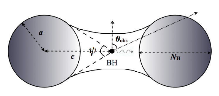
Figure 1: Assumed model geometry. The half-opening angle is given by $\frac{\pi-\psi}{2}$ and the inclination angle of the observer’s line of sight with the symmetry axis of the torus is given by $\theta_{\rm obs}$. The equatorial column density, $N_{\rm H}$, of the torus is defined by the diameter of the tube of the “doughnut”.

The inclination angle between the observer’s line of sight and the symmetry axis of the torus is given by $\theta_{\rm obs}$, where $\theta_{\rm obs}$ $=0^{\circ}$ corresponds to a face-on observing angle and $\theta_{\rm obs}$ $=90^{\circ}$ corresponds to an edge-on observing angle.

The equatorial column density, $N_{\rm H}$, is defined as the equivalent Hydrogen column density through the diameter of the tube of the torus (as indicated in Fig. 1). The actual line-of-sight column density is:

$$N_{\rm H,\ l.o.s.}=N_{\rm H}\left[1-\left(\frac{c}{a}\right)^{2}\cos^{2}{\theta_{\rm obs}}\right]^{\frac{1}{2}}.$$ (1)

The mean column density, integrated over all lines-of-sight through the torus, is $(\pi/4)$$N_{\rm H}$. The column density may also be expressed in terms of the Thomson depth: $\tau_{\rm T}=\frac{11}{9}N_{\rm H}\sigma_{\rm T}\sim 0.81N_{24}$ where $N_{24}$ is the column density in units of $10^{24}\rm\ cm^{-2}$. Note that this assumes that the abundance of He is 10% by number and that the number of electrons from all other elements aside from H and He is negligible. The mean number of electrons per H atom is $\frac{1}{2}(1+\mu)$, where $\mu$ is the mean molecular weight. In this case, $\mu=13/9$, for which $\frac{1}{2}(1+\mu)=11/9$.

The half-opening angle ($\frac{\pi-\psi}{2}$) of the torus is assumed to be $60^{\circ}$ (or $c/a=2$; see Fig. 1), corresponding to a scenario where there are equal numbers of unobscured and obscured AGN in the universe. The observed ratio of type 1 to type 2 AGN quoted in the literature varies widely (e.g. Treister, Krolik, & Dullemond 2008 reference values of type 1:type 2 AGN ratios that range from $\sim 2:3$ to $\sim 2:1$ and Elitzur 2008 refers to studies that find values of $\sim 3:7$ and $1:1$). Moreover, the ratio of type 1 to type 2 AGN is not necessarily the same as the ratio of unobscured to obscured AGN. The actual ratio is uncertain as it is dependent upon Seyfert classification definitions, but we have chosen a value that is consistent with observational findings reported in the literature. In future work, our calculations will be extended to include a range of opening angles.

We assume that the X-ray source emits isotropically and that the reprocessing material is uniform and essentially neutral (cold). Dynamics are not included in the Monte-Carlo code. Kinematic information can be approximated by convolving the Green’s functions or final output spectrum with a velocity function.

Calculation of each Green’s function involves multiple numerical calculations of the escape distances after each scattering and/or line-emission event. In order to calculate escape distances, we derived a quartic equation, $Z$, whose zeros yield the desired torus-boundary values as a function of the initial position and direction of a photon. In our Monte-Carlo code, the zeros of this equation were found using a bi-section method for a given tolerance, which we took to be $10^{-2}$, such that the solution yields a value in the range of $Z=0\pm 0.01$. This tolerance value was chosen to optimize accuracy and run-time of the Monte-Carlo code. Note that the initial photon position need not be inside the torus in order to obtain torus-boundary solutions, which is relevant in our code for finding the initial entry points of photons that are first injected into the torus. The function, $Z=0$, yields up to four solutions and therefore the appropriate solution must be selected in each case.

The Green’s functions have been computed over $N_{n}$ output bins of fractional Compton wavelength shift (in units of $h/m_{e}c$, where $h$ is the Planck constant, $m_{e}$ is the rest mass of the electron, and $c$ is the speed of light – see §3.5), for $N_{m}$ incident energies, $E_{m}$, and $N_{i}$ values of the equatorial column density through the structure, $N_{H,i}$. The Monte-Carlo output was further sorted into $N_{k}$ angular bins with cosine bin centers of $\mu_{k}$ (corresponding to the observer’s orientation relative to the axis of the torus). Using equal cosine intervals for the inclination angle bins ensures equal solid angles for each bin, thus ensuring that the numbers of photons in the bins with the smallest inclination angles are not photon-starved. Note that we do not need to retain the azimuthal escape angle information since the torus is axi-symmetric. We also utilize the polar symmetry about $\theta_{\rm obs}$ $=90^{\circ}$ by treating escape angles of $\theta_{\rm obs}$ and $180^{\circ}-$$\theta_{\rm obs}$ as equivalent. Thus there are $N_{k}$ Green’s functions (a “response” versus $N_{n}$ output bins) for each $E_{m}$ and $N_{H,i}$. Using interpolation, any of the Green’s functions can then be evaluated at any energy, and for any combination of $\theta_{\rm obs}$ and $N_{\rm H}$ on the grid. Storing the Green’s functions as a function of Compton wavelength shift (instead of energy) is essential for interpolation because they have sharp discontinuities at similar values of wavelength shift, not absolute energy (see §3.5).

Therefore, for a given arbitrary input spectrum $F_{\rm in}(E_{l},x_{1},x_{2},...)$ , where $x_{1,2...}$ are the parameters of the input spectrum, the transmitted and reprocessed spectrum, $F_{\rm R}(E_{i})$, can be computed on an arbitrary energy grid by numerically integrating the input spectrum over a Green’s function grid, interpolated on $E_{m}$, $G(E_{i},E_{m},N_{H,j},\mu_{k},g_{1},g_{2},...)$ (where the $g_{1,2...}$ are the other parameters of the Monte-Carlo model):

$$F_{\rm R}(E_{i},x_{1},x_{2},...,g_{1},g_{2},...)_{jk} = \sum_{(E_{l}\geq E_{i})}[G(E_{i},E_{l},N_{H,j},\mu_{k},g_{1},g_{2},...)\ F_{\rm in}(E_{l},x_{1},x_{2},...)\Delta E_{l}].$$ (2)

3.2 Zeroth-order Continuum

The continuum Green’s functions only include continuum photons that scattered at least once before escaping, and do not include the zeroth-order (straight-through) continuum photons that were not absorbed and that escaped without being scattered. The zeroth-order continuum for a given photon energy is simply

$$N_{\rm 0^{th}} = N_{\rm in}e^{-(\tau_{\rm a}+\tau_{\rm s})},$$ (3)

where $\tau_{\rm a}$ and $\tau_{\rm s}$ are the absorption and scattering optical depths along the line-of-sight, respectively, and $N_{\rm in}$ is the number of input photons per unit solid angle. Therefore the zeroth-order photon numbers can be computed numerically, independent of the Monte-Carlo results. The unscattered (zeroth-order) continuum can be added to the scattered continuum and the emission-line spectra calculated from the Green’s functions in order to obtain the net spectrum.

3.3 Compton Scattering and Photoelectric Absorption

A full exposition of Monte-Carlo methods for treating Compton scattering can be found in Pozdnyakov, Sobol, & Sunyaev (1983). The techniques for finite-Compton-depth transmission and reflection models have much in common with Monte-Carlo X-ray pure-reflection codes (e.g. George & Fabian 1991; Reynolds et al. 1994). We used the full differential Klein-Nishina Compton-scattering cross-section (used to generate the probability distribution to select the angle between initial and final photon directions), and the full Klein-Nishina angle-averaged Compton-scattering cross-section (which determines the probability of scattering for a given initial photon energy). See, for example, Pozdnyakov et al. (1983) or Coppi and Blandford (1990) for the full expressions. The total Klein-Nishina cross-section drops rapidly with increasing initial photon energy (relative to $m_{\rm e}c^{2}$) so the corresponding optical depth to scattering drops. Also, forward scattering dominates over back-scattering more and more as the initial photon energy increases (in the Thomson regime limit for low energies, forward and back-scattering are equally likely). In the electron rest frame, Compton scattering changes the energy of the incident energy of a photon, $E_{i}$, to $E_{f}=E_{i}/[1+(E_{i}/m_{\rm e}c^{2})(1-\cos{\alpha})]$, where $\alpha$ is the scattering angle relative to the initial photon direction, drawn from the differential cross-section distribution. A new azimuthal angle (about the new photon direction) is drawn from a uniform probability distribution. Since we are assuming that the torus is cold, the energy shifts in the electron rest frame are taken to be the same as those in the lab frame.

We utilized photoelectric absorption cross-sections for 30 elements as described in Verner & Yakovlev (1995) and Verner et al. (1996). Although these cross-section parameterizations are only valid up to 100 keV, the absorption cross-sections near 100 keV and at higher energies can be approximated by a simple power-law form and are orders of magnitude less than the values at the threshold energies (all $<10$ keV). Therefore, we extrapolated the total cross-section for energies above 100 keV using a power law with a slope equal to that in the $90-100$ keV interval. We used Anders and Grevesse (1989) elemental cosmic abundances in our calculations.

3.4 Fluorescent Emission Lines

We included fluorescent line emission in our Monte-Carlo code for Fe and Ni. Fluorescent lines from other cosmically-abundant elements (such as C, O, Ne, Mg, Si, and S) are less observationally relevant than those from Fe and Ni due to their small fluorescence yield and because lower-energy line photons have a greater probability of being absorbed before escaping the medium than higher-energy photons. See for example, Reynolds et al. (1994), and Matt, Fabian, & Reynolds (1997), who have calculated disk-reflection spectra, including all of these fluorescent lines. Although Ni K$\alpha$ line emission has been detected in a few sources (e.g. Molendi, Bianchi, & Matt 2003, and references therein), the fluorescent lines from Fe are by far the most important, due to the high fluorescence yield of Fe, and the relatively high abundance of Fe (the Ni solar abundance is only $\sim 3-6$% of the Fe abundance). Nevertheless, the fluorescent lines due to lighter elements will be included in future work since they can be important in “pure-reflection” spectra.

We therefore carried out a detailed treatment of the Fe K lines, explicitly including Fe K$\beta$ (at 7.058 keV) in addition to Fe K$\alpha$. For neutral Fe, the K$\alpha$ emission consists of two lines, K$\alpha_{1}$ at 6.404 keV and K$\alpha_{2}$ at 6.391 keV, with a branching ratio of 2:1 (e.g. see Bambynek et al. 1972). We treated these as a single line, but the two lines can easily be reconstructed from our Monte Carlo results. We additionally accounted for Ni K$\alpha$ emission at 7.472 keV (see Bearden 1967). We assumed Fe and Ni fluorescence yields of 0.347 and 0.414, respectively (see Bambynek et al. 1972) and an Fe K$\beta$ to Fe K$\alpha$ ratio of 0.135 (representative of the range of experimental and theoretical values discussed in Palmeri et al. 2003). These values, as well as the line energies, are subject to measurement and theoretical uncertainties. Additional discussion and a collection of results in the literature for these atomic parameters (including line energies) can be found in Kallman et al. (2004).

Our Monte-Carlo code calculates, using the relevant cross-sections, the probabilities for the photon to be absorbed by either an Fe K or Ni K shell, and in turn the probability for a fluorescent line to be created. We used K-shell absorption cross-sections and energies calculated by Verner et al. (1996) to calculate these probabilities. If Fe K shell fluorescence occurs, it is then determined if the emitted photon is an Fe K$\alpha$ or Fe K$\beta$ line photon. Each line photon is “labeled”, identifying it explicitly as Fe K$\alpha$, Fe K$\beta$, or Ni K$\alpha$. Once a fluorescent line photon is emitted, its passage through the medium is followed as it would be for any other photon (i.e., it is assigned a fresh starting energy and absorption, scattering, and escape are treated until the photon is absorbed or escapes). The Monte-Carlo output for the escaping fluorescent emission line photons consists of a single number for the zeroth-order line photons and an array containing the energy distribution of the scattered line photons (i.e., the Compton shoulder). Note that since the total photoelectric absorption cross-section at the energy of the Fe K$\beta$ line is less than that at the energy of the Fe K$\alpha$ line, the observed intensity ratio of Fe K$\beta$ to Fe K$\alpha$ may be larger than the Fe K$\beta$/Fe K$\alpha$ branching ratio.

3.5 Grid Parameters

In the present work, we calculated the Green’s functions for 28 values of the column density parameter, $N_{\rm H}$, in the range $10^{22}\rm\ cm^{-2}$ to $10^{25}\rm\ cm^{-2}$. The range in column density corresponds to a range in the Thomson depth of $\sim 0.0081-8.1$. The lower end of this range, where scattering becomes less important, ensures that there is no significant discontinuity when switching between spectra generated from the Green’s functions and those calculated from standard absorption models that do not include Compton scattering.

The output Green’s functions are stored in 10 $\theta_{\rm obs}$ bins that are equal in solid angle (see Table 1). For the current geometry with a half-opening angle of $60^{\circ}$, this corresponds to 5 bins that have lines-of-sight that intercept the torus (with $\theta_{\rm obs}$ between $60^{\circ}\rm\ and\ 90^{\circ}$) and 5 that have lines-of-sight that do not intercept the torus (with $\theta_{\rm obs}$ $<60^{\circ}$).

Table 1: $\theta_{\rm obs}$ Bin Boundaries. Bins 1–5 correspond to lines-of-sight that do not intercept the torus for the opening angle discussed here. Bins 6–10 correspond to lines-of-sight that intercept the torus.

Bin	$\cos{(\theta_{\rm obs,max})}$	$\cos{(\theta_{\rm obs,min})}$	$\theta_{\rm obs,min}$ (degrees)	$\theta_{\rm obs,max}$ (degrees)
1	0.9	1.0	0.00	25.84
2	0.8	0.9	25.84	36.87
3	0.7	0.8	36.87	45.57
4	0.6	0.7	45.57	53.13
5	0.5	0.6	53.13	60.00
6	0.4	0.5	60.00	66.42
7	0.3	0.4	66.42	72.54
8	0.2	0.3	72.54	78.46
9	0.1	0.2	78.46	84.26
10	0.0	0.1	84.26	90.00

Since we have assumed that the torus is comprised of cold matter, photons are always down-shifted in energy in our Monte-Carlo code. Thus, Green’s functions must be calculated for incident energies that are higher than the highest energy that we require for the final spectra (see §3.7). We use an upper incident photon energy of 500 keV, but this can easily be extended in future work. Below 5 keV, we adopted a different approach to explicitly calculate the Green’s functions because larger numbers of photons and input energies (and, therefore, longer run-times) are needed as absorption becomes more important. The procedure adopted for low energies is described in §3.6.

We have generated Green’s functions for 63 incident energies in the range of $5-500$ keV. Interpolation of these functions across different incident energies is problematic since there are sharp discontinuities at the boundaries of the energy distributions for each scattering. However, the shift in wavelength is linear and the maximum wavelength shift for a photon with a given incident energy that has been scattered $n$ times is $2n$ Compton wavelengths (see §3.3). Therefore, the Green’s functions have been stored in uniform bins in units of fractional Compton wavelength shift ($\Delta\lambda/\lambda_{\rm C}$) to facilitate interpolation since the discontinuities occur at the same place in these units regardless of incident energy. The value of $\Delta\lambda/\lambda_{\rm C}$ is calculated from the energy of the escaping photon ($E_{\rm esc}$) and that of the initial injected photon ($E_{\rm in}$) or, in the case of the emission lines, with respect to the zeroth order, rest-frame line energy:

$$\Delta\lambda/\lambda_{\rm C} = m_{\rm e}c^{2}(\frac{1}{E_{\rm esc}}-\frac{1}{E_{\rm in}})$$ (4)

The total number of Compton wavelengths included in each Green’s function is dictated by the largest number of scatterings experienced by any photon in a given Monte-Carlo run. For the parameter ranges considered in the present work, we did not need to account for more than 46 scatterings in the continuum. We set up 100 uniform bins per Compton wavelength; this corresponds, for example, to an energy resolution of $\sim 0.8$ eV at 6.4 keV and $\sim 140$ eV at 100 keV. At energies above $\sim 15$ keV the limited energy resolution of current – and likely near-future – detectors allows us to use much coarser bin sizes. In the $\sim 5.5-7.5$ keV output band we wish to treat the Fe K$\alpha$ and K$\beta$ line profiles with small enough bin sizes to be useful for future high-spectral resolution ($\sim 1$ eV) detectors. This does not require a fine mesh on the incident photon array because the line photons are generated in the medium at specific energies. Obtaining a fine resolution line profile requires only a sufficient number of photons in the line (and therefore in the incident spectrum), so that the photons can be distributed over a large number of output energy bins with sufficient statistical accuracy in each bin. Above 10 keV, for the majority of the Green’s functions, we have found that $10^{6}$ input photons are sufficient for the energy resolution we have chosen. However, at lower energies, especially near the Fe K edge, the Monte-Carlo runs have been performed with $10^{7}$ photons, in order to improve the statistical accuracy in the finer energy bins.

3.6 Low-Albedo, Low-Energy Regime

As the energy of the photons decreases, the absorption probability becomes increasingly higher and so the fraction of escaping photons decreases significantly. In order to obtain reliable escape fractions, larger input photon numbers must be injected into the torus at low energies. Moreover, the multitude of absorption edges below 10 keV would require carefully selected injection energies in order to achieve the desired energy resolution with sufficient accuracy accuracy (see §3.5). However, it is not, in fact, necessary to calculate the Green’s functions on such a fine energy grid when the energy is low enough that Compton scattering is in the Thomson regime. In that case, the total scattering cross-section is essentially independent of energy and, if absorption dominates over scattering, most of the escaping photons will be zeroth-order or once-scattered. Under these circumstances, the passage of photons through the torus depends only on the single-scattering albedo and not the initial energy. The (energy-dependent) single-scattering albedo is defined as the scattering cross-section as a fraction of the the total (absorption plus scattering) cross-section: $s\equiv\sigma_{\rm s}/(\sigma_{\rm a}+\sigma_{\rm s})$.

Using our Monte Carlo code, we can calculate the number of escaping photons for a relatively small set of albedo values and interpolate for any desired, arbitrary value of the albedo (see Fig. 2). Thus, to obtain the output for a given input photon energy, we can calculate the corresponding albedo for a given set of element absorption cross-sections at that energy and use that albedo value to obtain the escape fraction by interpolating the albedo-based Monte Carlo results. We note that if any of the element abundances is changed, the same albedo-based Monte-Carlo results can be used since only the correspondence between albedo and energy changes. In practice, we can calculate the zeroth-order photon numbers using Eq. 3 and use the interpolated Monte-Carlo results for the scattered photons. We can then use the numbers of escaping of photons in one of two ways. If the energy resolution involved in the application is such that the energy shifts are negligible, then we can simply place the zeroth-order and scattered photons in the same energy bin. At 5 keV the maximum energy shift after one scattering is $\sim 100$ eV, which is comparable to CCD-resolution. If the energy shifts cannot be neglected, we can use the Thomson differential cross-section to distribute the once-scattered photons over the correct energy bins.

We utilized Monte-Carlo runs for 17 values of $s$ between $10^{-4}$ and 1 for all of the grid values of $N_{\rm H}$ that were used in the full Monte-Carlo simulations (see §3.5), each starting with $10^{7}$ input photons. There is some overlap between the results from the albedo-based Monte-Carlo escape fractions and those from the Green’s functions that we calculated for $E_{\rm in}$ down to 5 keV, which allows confirmation of the self-consistency of the two methods (see §4).

Figure 2: The fraction of the number of escaping photons (including zeroth-order) relative to the number of input photons, versus the single-scattering albedo for $N_{\rm H}=10^{22}\rm\ cm^{-2}\ ({\it filled\ circles}),\ 10^{23}\ cm^{-2}\ ({\it open\ circles}),\ 10^{24}\ cm^{-2}\ ({\it squares}),\ and\ 10^{25}\ cm^{-2}$ (triangles), summed over all $\theta_{\rm obs}$ bins. These calculations are for the elastic-scattering regime, and do not depend on the input photon energy (see text for details).

3.7 Energy Range of Validity

The upper energy range of validity for the integrated spectra calculated from the Green’s functions depends on $N_{\rm H}$ and $\theta_{\rm obs}$, as well as on the shape of the input spectrum. At any particular energy value, the integrated spectrum includes contributions from Compton-down-scattered photons that had higher initial energies. In principle, an infinite number of scatterings could contribute to the total spectrum at a given energy. In practice, the intrinsic spectrum of an astrophysical source and the Klein-Nishina cross-section decrease with increasing energy. Therefore, only a finite number of scatterings contribute a significant fraction of the photons to the spectrum. We can quantify this by, for example, examining the number of scatterings that contribute to 90% or more of a given Green’s function. We calculated this number of scatterings as a function of $N_{\rm H}$ and $\theta_{\rm obs}$ from our Monte-Carlo results for the highest input energy ($E_{\rm in}$ $=500$ keV). This number, $n_{\rm max}$, increases from 1 to 6 as $N_{\rm H}$ increases from $10^{22}\rm\ cm^{-2}\ to\ 10^{25}\rm\ cm^{-2}$ for all $\theta_{\rm obs}$. For an initial energy of 500 keV, Compton down-scattering can reduce the output energy to $E_{f}=511[(511/500)+2n_{\rm max}]^{-1}$ keV. Since 500 keV is the largest value of $E_{\rm in}$ in our grids, this represents the upper limit of the range of validity of models based on these Green’s functions if the input spectrum extends beyond 500 keV. Fig. 3 shows this upper limit as a function of $N_{\rm H}$ for two values of $\theta_{\rm obs}$ (face-on and edge-on bins; see Table 1 ). We see that, for $N_{\rm H}$ $=10^{24}\rm\ cm^{-2}$, this upper limit corresponds to $\sim 169$ keV; for the largest column density ($N_{\rm H}$ $=10^{25}\rm\ cm^{-2}$), the upper limit is only $\sim 39$ keV. If the high-energy cut-off of the intrinsic spectrum of the astrophysical source being modeled is smaller or equal to 500 keV, the model is valid up to the cut-off energy. The range of high-energy cut-offs for the input spectra of AGN is poorly determined, but we note that non-blazar AGNs have rarely been detected above 500 keV (e.g. see Dadina 2008).

Figure 3: (a) Maximum number of scatterings experienced by 90% of the 500 keV input photons, as described in §3.7, versus $N_{\rm H}$, for the face-on (bin 1 – dotted curve) and edge-on (bin 10 –solid curve) $\theta_{\rm obs}$ bins (see Table 1 for the $\theta_{\rm obs}$ bin ranges). (b) Lowest final energy of 90% of the 500 keV input photons, versus $N_{\rm H}$, for the face-on (dotted curve) and edge-on (solid curve) $\theta_{\rm obs}$ bins (see Table 1 for the $\theta_{\rm obs}$ bin ranges).

4 Integrated Spectra

In the following, we discuss the results of integrating the Green’s functions described in §3, using a simple power-law input spectrum (flux $\propto E^{-\Gamma}\ \rm keV^{-1}$). Typical values of the photon index ($\Gamma$) of the intrinsic power-law for the majority of AGN range from 1.5 to 1.9 (e.g. Winter et al. 2008 and references therein). We present here examples using $\Gamma=1.5$ and 1.9 to represent this range. However, we note that one class of type 1 AGNs, NLS1s (narrow-line Seyfert 1 galaxies), tend to have steeper slopes, up to $\sim 2.5$. We do not assume an exponential cut-off above $\sim 100$ keV, as is often assumed in the literature. The functional form of a power-law with an exponential cut-off is not physical; in particular, thermal comptonization models do not predict curvature that can be modeled adequately with an exponential cut-off. More importantly, it is useful to obtain broad-band spectral results as a function of the empirical power-law slope without the extra complication of a cut-off energy. Then, if necessary, we can infer the results for an input spectrum with a high-energy cut-off. Furthermore, Compton-thick reprocessor models themselves, such as the one discussed here, introduce curvature in the high-energy spectra and therefore utilizing a simple power-law input spectrum allows us to assess this intrinsic curvature.

The broad-band spectrum for a given $N_{\rm H}$ and $\theta_{\rm obs}$ is created by first setting up an arbitrary energy grid for the integrated spectrum and, if the line-of-sight intercepts the torus, calculating the zeroth-order continuum for the given $\theta_{\rm obs}$ (see Eq. 1 and Eq. 3). Then the Green’s functions must be interpolated across the $E_{\rm in}$ table values for each point on the chosen energy grid. The interpolated Green’s functions are summed and convolved with the chosen input spectrum to produce the scattered spectrum (see Eq. 2), which can then be added to the zeroth-order continuum if the line-of-sight intercepts the torus, or to the intrinsic continuum if the line-of-sight does not intercept the torus.

The scattered contribution to the fluorescent lines is calculated in a similar manner to that of the scattered continuum. For the zeroth-order contribution to the fluorescent lines, the procedure is similar, but these photons are assigned to a single output energy bin, unique to each fluorescent line.

As described in §3.6, we have calculated a set of escape fractions for the low-energy, low-albedo regime, as a function of albedo ($s$) instead of $E_{\rm in}$. The integrated spectra presented here were calculated by simply assuming elastic scattering in this regime (the small energy shifts may be neglected for the present purposes – see §3.6). In this regime, each energy value on the chosen output grid must first be mapped to an albedo value. The escape fractions are then interpolated in albedo space, and then translated back to energy space and multiplied by the input spectrum. In Fig. 4, we compare the total, integrated spectrum derived from the primary, full, Monte-Carlo runs (dotted curve) with those obtained from the albedo-based escape fractions (solid curve) for the same input spectrum (a simple power-law with $\Gamma=1.9$) for $N_{\rm H}$ $=10^{24}\rm\ cm^{-2}$ for the case of the edge-on angle bin (bin 10; see Table 1). We see, in general, good agreement between the two sets of spectra up to $\sim 10$ keV. In all of the examples presented here we choose 5.5 keV as the cross-over energy between the albedo-based spectrum and the spectrum calculated from the primary, full, Green’s functions for the integrated spectra. We also point out that some of the structure around the Oxygen K edge seen in the albedo-based integrated spectra below $\sim 0.6$ keV for the edge-on $\theta_{\rm obs}$ bin is not physical, but a result of insufficient statistics.

Figure 4: Integrated scattered spectrum from the albedo-based Monte Carlo runs (solid curve), overlaid with the integrated scattered spectrum (dotted curve) from the full Monte-Carlo routine, for $N_{\rm H}$ $=10^{24}\ \rm cm^{-2}$ for the edge-on $\theta_{\rm obs}$ bin (bin 10 – see Table 1) for an input power-law continuum with $\Gamma=1.9$ (dashed line).

4.1 The Reprocessed Continuum

We have produced broad-band reprocessed spectra (including the Fe K$\alpha$, Fe K$\beta$, and Ni K$\alpha$ zeroth-order fluorescent lines and their Compton shoulders) for all of the grid values of $N_{\rm H}$ and $\theta_{\rm obs}$ for $\Gamma=1.5$ and 1.9 (a total of $28\times 10\times 2$ reprocessed spectra). Some of these spectra are illustrated in Fig. 5, which shows spectra for the face-on $\theta_{\rm obs}$ bin (bin 1 – dotted curves; see Table 1) and edge-on $\theta_{\rm obs}$ bin (bin 10 – solid curves; see Table 1) for $N_{\rm H}$ $=5\times 10^{23}\rm\ cm^{-2}\ ({\it top\ left}),\ 10^{24}\rm\ cm^{-2}\ ({\it top\ right}),\ 5\times 10^{24}\rm\ cm^{-2}\ ({\it bottom\ left}),\ and\ 10^{25}\rm\ cm^{-2}\ ({\it bottom\ right})$ for an input power-law continuum with $\Gamma=1.9$ (dashed line). The zeroth-order spectrum for the edge-on $\theta_{\rm obs}$ bin is also shown (dot-dashed curves) for each $N_{\rm H}$. Note again that, for the edge-on angle bin, the spectrum below $\sim 0.6$ keV is subject to significant statistical error and should be interpreted with caution. For the five angle bins that intercept the torus, ($\theta_{\rm obs}$ $\geq 60^{\circ}$ – see Table 1), the reprocessed spectrum includes the zeroth-order (transmitted) continuum as well as the scattered continuum. For the five non-intercepting angle bins ($\theta_{\rm obs}$ $<60^{\circ}$), the reprocessed spectrum includes only the scattered continuum. Therefore, in order to obtain the total observed spectrum in the non-intercepting angle bins, we must add the intrinsic continuum to the reprocessed spectra. It should be noted that in Fig. 5 and in subsequent figures we show only the reprocessed spectrum for the non-intercepting angles in order to directly compare spectral features for face-on and edge-on angle bins. From Fig. 5 we see that the Compton hump, as expected, begins to appear for column densities of $10^{24}\rm\ cm^{-2}$ and higher and is stronger for the edge-on (solid) spectra since the photons that are scattered into the edge-on angle bin in general pass through a larger Thomson depth than those that are scattered into the face-on angle bin (dotted). At low energies, although the continuum is diminished, we do not see a complete extinction of the spectrum. In contrast, a pure-absorption model or a spherical Compton-thick model would predict a stronger suppression of the low-energy photons (e.g. Leahy & Creighton 1993; Yaqoob 1997), especially for column densities of $10^{24}\rm\ cm^{-2}$ and higher. Our torus model instead results in a non-negligible number of photons being scattered into the line-of-sight at low energies, even for the edge-on observing angle of a high-$N_{\rm H}$ torus, due to the smaller line-of-sight column densities towards the surface of the torus. At high energies, we find that the spectra for the face-on angle bin cut off at lower energies than those for the edge-on angle bin. This is due to the diluting effect of the zeroth-order contribution to the reprocessed spectra in the angle bins that intercept the torus. For $N_{\rm H}$ less than $\sim 5\times 10^{24}\rm\ cm^{-2}$, the edge-on reprocessed spectra are dominated by the zeroth-order photons. However, we find that, for high $N_{\rm H}$ values (greater than $\sim 5\times 10^{24}\rm\ cm^{-2}$) even the edge-on high-energy spectra are suppressed (since the zeroth-order photons no longer dominate).

To illustrate the difference in the relative amplitude of the scattered spectra as a function of observing angle, we show in Fig. 6 the ratio of the scattered-to-intrinsic continuum at a single energy (6.4 keV) for an input power-law continuum with $\Gamma=1.9$, versus $\theta_{\rm obs}$. These ratios are shown for $N_{\rm H}$ $=5\times 10^{23}\rm\ cm^{-2}\ ({\it dot-dashed\ curve}),\ 8\times 10^{23}\rm\ cm^{-2}\ ({\it dashed\ curve}),\ 2\times 10^{24}\rm\ cm^{-2}\ ({\it dotted\ curve}),\ and\ 10^{25}\rm\ cm^{-2}\ ({\it solid\ curve})$. For all values of $N_{\rm H}$, the ratios show little dependence on the inclination angle for values of $\theta_{\rm obs}$ that do not intercept the torus. In the Thomson-thin regime, as would be expected, there is little distinction in the ratio of the reprocessed-to-intrinsic continuum between intercepting and non-intercepting lines of sight, in contrast with the behavior for larger column densities.

Figure 5: Total integrated spectra for an input power-law continuum with $\Gamma=1.9$ (dashed line). Spectra for the face-on $\theta_{\rm obs}$ bin (bin 1 – dotted curves; see Table 1) and edge-on $\theta_{\rm obs}$ bin (bin 10 – solid curves; see Table 1) are shown for $N_{\rm H}$ $=5\times 10^{23}\rm\ cm^{-2}\ ({\it top\ left}),\ 10^{24}\rm\ cm^{-2}\ ({\it top\ right}),\ 5\times 10^{24}\rm\ cm^{-2}\ ({\it bottom\ left}),\ and\ 10^{25}\rm\ cm^{-2}\ ({\it bottom\ right})$. The zeroth-order spectrum for the edge-on $\theta_{\rm obs}$ bin is shown (dot-dashed curves) for each $N_{\rm H}$. Note that, for the edge-on angle bin, the spectrum below $\sim 0.6$ keV is subject to significant statistical error and should be interpreted with caution.

Figure 6: The ratio of the number of scattered photons at 6.4 keV that have escaped from the torus to the incident continuum photons at 6.4 keV, versus $\theta_{\rm obs}$ for $N_{\rm H}$ $=5\times 10^{23}\rm\ cm^{-2}\ ({\it dot-dashed\ curve}),\ 8\times 10^{23}\rm\ cm^{-2}\ ({\it dashed\ curve}),\ 2\times 10^{24}\rm\ cm^{-2}\ ({\it dotted\ curve}),\ and\ 10^{25}\rm\ cm^{-2}\ ({\it solid\ curve})$.

Thus far, we have focused on the reprocessed spectra that result from a power-law input spectrum with $\Gamma=1.9$. We have confirmed that the chosen value of the spectral index has little effect on the general behavior of the integrated, reprocessed continuum. However, we note that for the scattered continuum, the amplitude of the Compton hump relative to the spectral flux below 10 keV is larger for flatter incident continua. We find that the maximum ratio of the scattered to incident flux (i.e., at the peak of the Compton hump) for $\Gamma=1.5$ is $\sim 25$% higher than the same ratio for $\Gamma=1.9$ for $N_{H}=10^{25}\ \rm cm^{-2}$ and the face-on angle bin (bin 1, Table 1). For the edge-on angle bin and the same column density, the corresponding enhancement of the Compton hump for $\Gamma=1.5$ relative to $\Gamma=1.9$ is $\sim 35$%.

4.1.1 Comparison with PEXRAV

It is common practice is to use a disk-reflection model (in particular, pexrav in XSPEC – see Magdziarz & Zdziarski 1995) to attempt to imitate scattering in the torus or other non-disk geometry. The disk geometry is clearly incongruent to the geometry of the distant-matter reprocessor and therefore the derived parameters are not relevant or physical. It is useful to directly compare the reprocessed spectra from the angle bins that do not intercept the torus with spectra obtained with pexrav in order to assess the effect on spectral-fitting results reported in the literature. The key parameters of the disk-reflection model are the inclination angle of the disk normal relative to the observer’s line-of-sight, and the so-called “reflection fraction”, $R$. The latter is a multiplication factor for the reflected spectrum normalization obtained from a semi-infinite, neutral disk illuminated by a non-varying X-ray point-source continuum. Thus, if the disk-reflection model is applied to a situation for which the disk geometry is not appropriate, the value of $R$ that is obtained to force a fit to data no longer has a meaningful interpretation. Nevertheless, the results of forced disk-reflection fits to obscured AGN abound in the literature.

Fig. 7 shows a comparison of an integrated spectrum obtained from our Monte-Carlo torus results (for an input spectrum with $\Gamma=1.9$ and $N_{\rm H}$ $=10^{25}\rm\ cm^{-2}$) with spectra obtained with the pexrav model in XSPEC. The torus spectrum is shown for the face-on $\theta_{\rm obs}$ bin (bin 1; dotted curve). Overlaid are the pexrav results for the smallest value of $\theta_{\rm obs}$ allowed by that model ($18^{\circ}$) with two reflection fraction values ($R=1$ and $R\sim 0.16$) as well as for $\theta_{\rm obs}$ $=60^{\circ}$ with $R=1$. It can be seen that, relative to the intrinsic power-law, the reflection continuum from our torus model is significantly weaker than both of the pexrav components with $R=1$. The value of $R\sim 0.16$ simply aligns the face-on, $R=1$ pexrav component approximately with the torus component at the position of the Fe K edge. However, the detailed shape of the soft X-ray continuum and the Compton hump from the torus model are different compared to the pexrav spectra. These differences are due to geometry effects and are significant enough to potentially impact fitting results for high signal-to-noise data. Even for lower signal-to-noise data, our results show that, for the angle bin that gives the largest reflection spectrum from the torus (i.e., face-on), the reflected continuum is suppressed by a factor $\sim 6$ compared to a disk geometry.

The difference between the Compton-thick reflection spectrum from our torus model and that from a disk is substantial. This is due to several effects. One is that when the torus becomes Compton-thick, half of the photons reflected from its surface are directed away from the observer. The projection effects due to the curved toroidal surface, and re-entry of some of the reflected photons into the torus also play a role. The fact that face-on viewing angles in the adopted geometry disfavor forward and back-scattered photons contributes to angle-dependent reflection via the differential scattering cross-section. A more significant factor is that the amplitude of the reflection spectrum depends critically on the angle of reflection relative to the local normal on the toroidal surface. As this angle varies over the toroidal surface between $90^{\circ}$ and the complement of the half-opening angle (i.e., $30^{\circ}$ for a half-opening angle of $60^{\circ}$) for the face-on orientation, the reflection spectrum amplitude varies from zero to some value that is less than that for a $0^{\circ}$ reflection angle. The net reflection spectrum amplitude will then be a function of the range in reflection amplitude integrated over all reflection angles over the toroidal surface. Thus, the virtually universal practice of interpreting the so-called “reflection-fraction” as a literal covering factor, or solid angle, from fitting disk-reflection spectra is erroneous. We have shown that even though our torus subtends the same solid angle at the X-ray source as a disk ($2\pi$), the reflection spectrum amplitude from the torus is a factor of $\sim 6$ less than that from the disk. Even different toroidal geometries will give different amplitudes for the Compton-thick reflection spectra for the same torus half-opening angle. For example the spherical-torus geometry of Ghisellini et al. (1994) and Ikeda et al. (2009) will give different reflection continuum amplitudes because the reflection angle relative to a local normal anywhere on the reflecting surface is constant. For the particular parameters adopted by Ikeda et al. (2009), a half-opening angle of $60^{\circ}$ gives a reflection angle of $\sim 30^{\circ}$ so in that case the reflection spectrum will be stronger than that in our models.

Changing the opening angle of the torus does not change our conclusion about the weakness of Compton-thick reflection for our geometry (compared to that for a disk). Increasing the torus open angle decreases the solid angle subtended at the X-ray source and thus reduces the reflection spectrum. Decreasing the opening angle of the torus increases the magnitude of the reflection spectrum, but this is countered by a decrease due to the increase in the average angle of reflection. A half-opening angle somewhere between $30^{\circ}$ and $45^{\circ}$ will maximize the amplitude of the reflection spectrum but it will never be greater than a factor of $2$ relative to the half-opening angle of $30^{\circ}$ (e.g. see Ikeda et al. 2009). Although a direct comparison between the Compton-thick reflection spectrum from the non-intercepting angle bins of our torus model and that from a disk is simple, a comparison for obscured lines-of-sight is not straight-forward. For inclination angles that intercept the reprocessor it is not possible to assign a useful meaning to fitted values of $R$ since the reprocessed spectrum is typically modeled in the literature by an ad hoc combination of pure absorption plus disk-reflection.

Figure 7: Comparison of an integrated spectrum obtained from our Monte-Carlo torus results with those obtained with the pexrav model in XSPEC for an input power-law spectrum with $\Gamma=1.9$ (dashed line) and $N_{\rm H}$ $=10^{25}\rm\ cm^{-2}$. The torus spectrum is shown for the face-on $\theta_{\rm obs}$ bin (bin 1 – dotted; see Table 1). Overlaid are the pexrav results for the smallest value of $\theta_{\rm obs}$ allowed by the model ($18^{\circ}$) for two values of the reflection normalization, $R=1$ and $R\sim 0.16$. Also shown is the spectrum obtained with pexrav, for $\theta_{\rm obs}$ $=60^{\circ}$ and $R=1$.

4.2 The Fe K$\alpha$ Emission Line

4.2.1 Fluorescent Line Equivalent Widths

The equivalent widths (EWs) of the fluorescent lines are an important diagnostic of the material out of the line-of-sight. Observational measurements of the EWs of the fluorescent Fe K$\alpha$ emission line in the literature generally refer to the zeroth-order emission only, since the line is typically fitted with a Gaussian. The scattered flux (i.e., the Compton shoulder, which can carry up to 40% of the zeroth-order flux – see §4.2.2) is generally not fitted (usually because it is not detected), or, if it is fitted, a separate EW is quoted. Yet these zeroth-order line EWs are often compared to theoretical predictions that include all of the line photons (zeroth-order and scattered; e.g. Leahy & Creighton 1993, Ghisellini et al. 1994, Ikeda et al. 2009). In Fig. 8, we show the zeroth-order EWs of the Fe K$\alpha$ line as a function of the column density of the torus, $N_{\rm H}$, since it is the zeroth-order emission that is observationally-relevant for the main peak of the line. The lower curves show the results for the non-intercepting angle bins, with ascending $\theta_{\rm obs}$ bins from top to bottom, and the upper curves show the results for the intercepting angle bins, with ascending $\theta_{\rm obs}$ bins from bottom to top.

It can be seen in Fig. 8 that, for $N_{\rm H}$ less than $\sim 5\times 10^{22}\ \rm cm^{-2}$, inclination-angle effects are not important (as would be expected for the Thomson-thin limit). Overlaid on Fig. 8 is the theoretical Thomson-thin limit (dashed line), given by

$$EW_{\rm Fe-K\alpha} = 785\ \left(\frac{\Delta\Omega}{4\pi}\right)\ \left(\frac{\omega_{K}}{0.347}\right)\ \left(\frac{\rm A_{\rm Fe}}{4.68\times 10^{-5}}\right)\ \left(\frac{\sigma_{0}}{3.37\times 10^{-20}\rm\ cm^{2}}\right)\ \left(\frac{3.57}{\Gamma+\alpha-1}\right)\ \left(0.8985\right)^{(\Gamma-1.9)}\ N_{24}\ \rm eV$$ (5)

(see Yaqoob et al. 2001 for details, but note that Eq. 5 differs from the corresponding equation in Yaqoob et al. 2001 since the latter erroneously included the total cross-section at the Fe K edge threshold, instead of the K-shell cross-section only).

The quantity $(\Delta\Omega/4\pi)$ is the solid angle of the line-emitting matter subtended at the X-ray source. For the torus, $N_{24}=(\pi/4)(N_{\rm H}/10^{24}\rm\ cm^{-2})$ is the column density averaged over all incident photon angles. The K-shell fluorescence yield is given by $\omega_{K}$ and $A_{\rm Fe}$ is the Fe abundance relative to Hydrogen. The quantity $\sigma_{0}$ is the Fe K shell absorption cross-section at the Fe K edge, and $\alpha$ is the power-law index of the cross-section as a function of energy. We fitted photoelectric K-shell absorption cross-section data from Verner et al. (1996) tables with a simple power-law and obtained

$$\sigma_{\rm Fe-K}(E)=\sigma_{0}\left(\frac{E}{E_{K}}\right)^{-2.67}\times 10^{-20}\ \rm cm^{2}\ per\ atom$$ (6)

for $E\geq E_{K}$, giving $\alpha=2.67$ and $\sigma_{0}=3.37$, where $E_{K}=7.124$ keV in Verner et al. (1996).

Figure 8: The Fe K$\alpha$ line equivalent width versus $N_{\rm H}$ for $\Gamma=1.9$ as calculated from the Monte-Carlo code, and the theoretical Thomson-thin limit (dashed line). Curves are shown for each of the 10 $\theta_{\rm obs}$ bins (see Table 1). The lower set of curves corresponds to bins 1–5 (lines-of-sight that do not intercept the torus) and the upper set of curves correspond to bins 6–10 (lines-of-sight that intercept the torus). The solid curves correspond to the two boundary $\theta_{\rm obs}$ bins (bins 1, 5, 6, and 10; see Table 1) for both intercepting and non-intercepting cases.

In the limit of small $N_{\rm H}$, the relation between the EW and $N_{\rm H}$ is linear, for all observing angles, regardless of the value of $\Gamma$. The slope of this relation depends only on the element abundance, $\Gamma$, and $\Delta\Omega/4\pi$. It can be seen in Fig. 8 that inclination-angle effects begin to appear even for $N_{\rm H}$ $\sim 10^{23}\rm\ cm^{-2}$.

For inclination angles that do not intercept the torus, the EW peaks between $\sim 5\times 10^{23}\rm\ cm^{-2}\ and\ 10^{24}\ cm^{-2}$, then decreases by $\sim 50$% of this peak value at $N_{\rm H}$ $=10^{25}\ \rm cm^{-2}$. The peak value for the EW of the Fe K$\alpha$ line, for $\Gamma=1.9$, is $\sim 70$ eV (for the case of $\Gamma=1.5$, the peak value is $\sim 85$ eV). The decrease in the EWs at the higher values of $N_{\rm H}$ is due to the fact that the absolute number of escaping line photons decreases, partly because more escaping photons appear in the Compton shoulder (see §4.2.2). Additionally, the total continuum is dominated by the intrinsic continuum, which is not affected by the torus at these inclination angles. Fig. 8 shows that the limiting Fe K$\alpha$ line EW for Compton-thick reflection can be as little as $\sim 30$ eV, a factor of $\sim 5-6$ less than that expected from a face-on disk (e.g. see George & Fabian 1991). The reasons for this are the same as those discussed for the relative weakness of the Compton-thick reflection continuum (§4.1.1). The spherical-torus geometry adopted by Ghisellini et al. (1994) and Ikeda et al. (2009) can yield larger values of the limiting Fe $K\alpha$ line EW for Compton-thick reflection for the same half-opening angle as in our calculations. Again this is due to the same reasons that their geometry can give a larger reflection continuum, as discussed in §4.1.1.

Fig. 9 shows the Fe K$\alpha$ line EW versus $\theta_{\rm obs}$ for $\Gamma=1.9$ and $N_{\rm H}$ $=5\times 10^{23}\rm\ cm^{-2}\ ({\it dot-dashed}),\ 8\times 10^{23}\rm\ cm^{-2}\ ({\it dashed}),\ 2\times 10^{24}\rm\ cm^{-2}\ ({\it dotted}),\ and\ 10^{25}\rm\ cm^{-2}\ ({\it solid})$. For the non-intercepting angle bins the EW is not very sensitive to $\theta_{\rm obs}$, but the face-on EW can be $\sim 30$% higher than the EW for the largest non-intercepting value of $\theta_{\rm obs}$ when the continuum at 6.4 keV is dominated by one Compton scattering (i.e., $N_{H}\sim 1-2\times 10^{24}\ \rm cm^{-2}$). This is because the form of the differential scattering cross-section in the Thomson regime preferentially produces more forward-scattered and back-scattered photons compared to those with intermediate scattering angles. In our toroidal geometry this means that there are less continuum photons scattered into the face-on angle bin than those with larger inclination angles when only one scattering dominates. Since the zeroth-order Fe K$\alpha$ line photons are emitted isotropically, the net result is an enhanced EW for smaller inclination angles in the column-density regime for which the Thomson depth is of order unity. For the torus-intercepting angle bins, the EWs of the lines increase as $N_{\rm H}$ increases up to $\sim 3\times 10^{24}\rm\ cm^{-2}$ since the zeroth-order continuum, which dominates the continuum at these column densities, decreases due to an increasing line-of-sight column density (see Fig. 8). Above $\sim 3\times 10^{24}\rm\ cm^{-2}$, it is the scattered continuum that begins to dominate the spectrum. Since both the absolute flux of the emission lines and that of the scattered continuum effectively decrease at a similar rate as $N_{\rm H}$ increases, the EWs of the lines saturate at high $N_{\rm H}$, where the scattered continuum dominates. The EWs obtained for the intercepting angle bins are very sensitive to $\theta_{\rm obs}$ for $N_{\rm H}$ greater than $2\times 10^{23}\rm\ cm^{-2}$ due to the diminishing zeroth-order contribution to the continuum; at a given $N_{\rm H}$ the EW becomes larger as $\theta_{\rm obs}$ increases (as seen in Fig. 9). For the edge-on angle bin, the maximum values of the Fe K$\alpha$ EW are $\sim 3.8$ keV and $\sim 2.5$ keV for $\Gamma=1.5$ and 1.9, respectively.

Figure 9: The Fe K$\alpha$ line equivalent width versus $\theta_{\rm obs}$ for $\Gamma=1.9$ and $N_{\rm H}$ $=5\times 10^{23}\rm\ cm^{-2}\ ({\it dot-dashed}),\ 8\times 10^{23}\rm\ cm^{-2}\ ({\it dashed}),\ 2\times 10^{24}\rm\ cm^{-2}\ ({\it dotted}),\ and\ 10^{25}\rm\ cm^{-2}\ ({\it solid})$.

We find that smaller values of $\Gamma$ yield larger values of the Fe K$\alpha$ EW; this is expected as there are relatively more photons in the continuum above the Fe K edge for flatter spectra. Fig. 10 shows the ratio of the Fe K$\alpha$ line equivalent width for $\Gamma=1.5$ to the corresponding equivalent width for $\Gamma=1.9$, versus $N_{\rm H}$, for each of the inclination-angle bins (see Table 1). In the Compton-thick regime, the ratio of the equivalent widths for the non-intercepting angle bins can be as large as 1.3 and for the intercepting bins it can be as large as 1.6.

Figure 10: Ratio of the Fe K$\alpha$ line equivalent width for $\Gamma=1.5$ to the corresponding equivalent width for $\Gamma=1.9$, versus $N_{\rm H}$. Curves are shown for each of the 10 $\theta_{\rm obs}$ bins (see Table 1). The lower set of curves corresponds to bins 1–5 (lines-of-sight that do not intercept the torus) and the upper set of curves correspond to bins 6–10 (lines-of-sight that intercept the torus). The solid curves correspond to the two boundary $\theta_{\rm obs}$ bins (bins 1, 5, 6, and 10; see Table 1) for both intercepting and non-intercepting cases.

The EW versus $N_{\rm H}$ curves have an explicit dependence on the assumed opening angle of the torus. This is because different opening angles correspond to different solid angles subtended by the torus at the source and to different projection-angle effects. In the Thomson-thin regime, this dependence is linear (see Eq. 5). In the Compton-thick regime, there is a more complicated dependence that must be determined by additional Monte-Carlo simulations and will be the subject of future investigation (see Ikeda et al. 2009 for discussion in the context of a different toroidal geometry).

4.2.2 Fe K$\alpha$ Line Compton Shoulder

In addition to the zeroth-order core of the Fe K$\alpha$ emission line, the shape and relative magnitude of the Compton shoulder are also sensitive to the properties of the reprocessor. Evidence for the Compton shoulder has already been found in some sources (e.g. see Iwasawa, Fabian, & Matt 1997; Matt 2002; Kaspi et al. 2002; Watanabe et al. 2003; Yaqoob et al. 2005), although detections of the Compton shoulder to date have been ambiguous. Future detectors, such as X-ray calorimeters, will be able to measure the line profile structure in more detail than is currently possible.

In this section we discuss the relative strength of the scattered component of the Fe K$\alpha$ emission line (i.e., the Compton shoulder) with respect to the zeroth-order line component and the continuum. Fig. 11 shows ratio plots of the total number of scattered Fe K$\alpha$ line photons to zeroth-order Fe K$\alpha$ line photons versus $N_{\rm H}$. The ratios are shown for an input power-law continuum with $\Gamma=1.9$, for two $\theta_{\rm obs}$ bins (face-on – bin 1 – dotted curve and edge-on – bin 10 – solid curve; see Table 1). Note that, for $N_{\rm H}$ $<10^{23}\rm\ cm^{-2}$, these ratios are affected by small-number statistics and should be interpreted with caution. The general trend is that the ratios increase as $N_{\rm H}$ increases, up to a column density between $10^{24}\rm\ cm^{-2}\ and\ 5\times 10^{24}\ cm^{-2}$, since the Thomson depth is increasing. At higher column densities, the ratio curves turn over (and begin to decrease for some of the highest $\theta_{\rm obs}$ bins), as a greater fraction of scattered line photons are absorbed. The maximum of the ratio for angle bin 1 (face-on) is $\sim 0.3$ and for angle bin 10 (edge-on) is $\sim 0.4$. This means that the zeroth-order line may contain as little as 71% of the total line flux.

Although the energy interval of the first Compton scattering (6.24–6.4 keV) includes photons from multiple scatterings, in real data it would be impossible to isolate the once-scattered photons. Nevertheless, it is the 6.24–6.4 keV interval that is relevant for the observationally-measured Compton shoulder, which therefore includes contributions from more than one scattering. Line flux below 6.24 keV is difficult to distinguish from the continuum. At the lowest column densities, essentially all of the scattered line photons are in the first-order. We found from our Monte-Carlo results that as $N_{\rm H}$ increases, the ratio of the total number of scattered line photons in the 6.24–6.4 keV interval (i.e., the measured Compton shoulder) to the total number of scattered line photons is $\sim 0.85$, regardless of $\theta_{\rm obs}$ and $\Gamma$. The general behavior of the ratio of the scattered to the zeroth-order line photon is independent of $\Gamma$. This is expected as we are considering ratios of numbers of line photons, which do not depend on the intrinsic continuum. Detailed results concerning the shape of the Compton shoulder will be presented in future work.

Figure 11: The ratios of the total number of scattered Fe K$\alpha$ line photons to the number of zeroth-order Fe K$\alpha$ line photons versus $N_{\rm H}$. Ratios are shown for an input power-law continuum with $\Gamma=1.9$, for the face-on (bin 1 – dotted curve; see Table 1) and edge-on (bin 10 – solid curve; see Table 1) $\theta_{\rm obs}$ bins. Note that for $N_{\rm H}$ $<10^{23}\rm\ cm^{-2}$, these ratios are affected by small number statistics and should be interpreted with caution.

5 Summary

We have calculated Green’s functions that may be used to produce spectral-fitting routines to model the putative neutral toroidal X-ray reprocessor in AGNs for an arbitrary input spectrum. The absolute size of the structure does not affect the reprocessed spectrum so our results can be used to model any distant-matter, cold, toroidal structure in the central engine, from the optical broad-line region (BLR) and beyond. A doughnut-shaped torus geometry has been employed and the model has been calculated for a single half-opening angle of $60^{\circ}$ and is valid for column densities in the range $10^{22}\rm\ cm^{-2}\ and\ 10^{25}\rm\ cm^{-2}$. The upper end of the column density range likely satisfies the majority of current observational needs but can easily be extended in the future. Our calculations are fully relativistic and valid up to 500 keV if the intrinsic incident spectrum has a cut-off below this energy. For intrinsic spectra that extend beyond 500 keV we have assessed in detail the range of validity of the calculations. However, the Green’s function approach enables this energy range to be easily extended with further Monte Carlo runs. We find that our adopted geometry produces significant flux in the soft X-ray band even for Compton-thick column densities along edge-on lines of sight. Such soft flux can be observationally important and could manifest itself as complex absorption in the soft X-ray band. The Monte-Carlo code treats the reprocessed continuum as well as the three most important fluorescent emission lines (Fe K$\alpha$, Fe K$\beta$, and Ni K$\alpha$) with sufficient detail such that the results are applicable to observations obtained by current and planned X-ray instrumentation.

The reprocessed continuum and fluorescent line emission due to Fe K$\alpha$, Fe K$\beta$, and Ni K$\alpha$ are treated self-consistently in our calculations, eliminating the need for ad hoc modeling that is currently common practice. We have found that the reflection spectrum from a Compton-thick face-on torus that subtends a solid angle of $2\pi$ at the X-ray source is factor of $\sim 6$ weaker than that expected from a Compton-thick, face-on disk, even though the latter subtends the same solid angle. This is a very significant difference and emphasizes the universal misinterpretation of the so-called “reflection fraction” (defined in terms of the disk geometry) as a literal solid angle (as a fraction of $2\pi$). The relative strength of the reflection continuum very critically depends on geometry because it is affected by the angle of reflection integrated over the surface of the reprocessor. Even different toroidal geometries give different amplitudes of the reflected spectrum for the same solid angle subtended at the X-ray source. A direct comparison of our Compton-thick reflected continua with the disk-reflection model pexrav, shows that not only is the amplitude substantially different, but the shape of the soft X-ray spectrum and the shape and relative amplitude of the $\sim 10-30$ keV “Compton-hump” are different enough to have observational consequences. Since the Fe K$\alpha$ line EW is physically related to the reflection continuum, it is also correspondingly weaker than the Fe K$\alpha$ line EW expected from a disk. For our Compton-thick torus observed face-on, the Fe K$\alpha$ line EW can be as little as $\sim 30$ eV. Curves of EW of the Fe K$\alpha$ line versus $N_{\rm H}$ such as those presented in this work can be generated for arbitrary input spectra and can be used as an important diagnostic of the reprocessor. The effects of geometry and inclination become apparent at column densities larger than $\sim 2\times 10^{23}\rm\ cm^{-2}$. Our calculations are detailed enough to allow orientation effects to be modeled in the X-ray spectra, providing more quantitative tests of the unified model.

Spectral-fitting routines are generally characterized by a trade-off between speed and model detail. A variety of spectral-fitting routines may be constructed based on our results, depending on the desired speed and application. By design, these routines could be combined with other models in spectral fitting packages.

Acknowledgments
The authors thank Shinya Ikeda, Hisamitsu Awaki, and Yuichi Terashima for fruitful discussions. We thank Andrzej Zdziarski for carefully reviewing the manuscript and for constructive comments. Partial support from NASA grants NNG04GB78A (KM, TY) and NNX09AD01G (TY) is acknowledged.

References

- [1] Anders E., Grevesse N., 1989, Geochimica et Cosmochimica Acta 53, 197
- [2] Antonucci R. R. J., Miller J. S., 1985, ApJ, 297, 621
- [3] Arnaud K. A., 1996, in Astronomical Data Analysis Software and Systems V, ed. G. Jacoby, J. Barnes (Astronomical Society of the Pacific), Conference Series, Vol. 101, p. 17
- [4] Awaki H., Hideyo K., Yuzuru T., Koyama K., 1991, PASJ, 43, 195
- [5] Bambynek W., Crasemann B., Fink R. W., Freund H.-U., Mark H., Swift C. D., Price R. E., Rao P. V., 1972, Rev. Mod. Phys., 44, 716
- [6] Bearden J. A., 1967, Rev. Mod. Phys., 39, 78
- [7] Bianchi S., La Franca F., Matt G., Guainazzi M., Jiménez-Bailón E., Longinotti A. L., Nicastro F., Pentericci L., 2008, MNRAS, 389, 52
- [8] Braito V., Della Ceca R., Piconcelli E. et al. 2004, A&A, 420, 79
- [9] Chartas G., Eracleous M., Dai X., Agol E., Gallagher S., 2007, ApJ, 661, 678
- [10] Coppi P. S., Blandford R. D., 1990, MNRAS, 245, 453
- [11] Dadina M., 2008, A&A, 485, 417
- [12] Done C., Madejski G. M., Smith D. A., 1996, ApJ, 463, 63
- [13] Elitzur M., 2008, NewAR, 52, 274
- [14] Gallagher S. C., Brandt W. N., Chartas G., Priddey R., Garmire G. P., Sambruna R. M., 2006, ApJ, 644, 709
- [15] Gaskell C. M., Goosmann R. W., Klimek E. S., 2008, MmSAI, 79, 1090
- [16] George I. M., Fabian A. C., 1991, MNRAS, 249, 352
- [17] Ghisellini G., Haardt F., Matt G., 1994, MNRAS, 267, 743
- [18] Guainazzi M., Matt G., Perola G. C., 2005, A&A, 444, 119
- [19] Guilbert P. W., Rees M. J., 1988, MNRAS, 233, 475
- [20] Haardt F., Maraschi L., 1991, ApJ, 380, 51
- [21] Houck J. C., Denicola L. A., 2000, ASPC, 216, 591
- [22] Illarionov A., Kallman T., McCray R., Ross, R., 1979, ApJ, 228, 279
- [23] Ikeda S., Awaki H., Terashima Y., 2009, ApJ, 692, 608
- [24] Iwasawa K., Fabian A. C., Matt G., 1997, MNRAS, 289, 443
- [25] Jiang P., Wang J. X., Wang T. G., 2006, ApJ, 644, 725
- [26] Jiménez-Bailón E., Piconcelli E., Guainazzi M., Schartel N., Rodr guez-Pascual P. M., Santos-Lleó M., 2005, A&A, 435, 449
- [27] Kallman T. R., Palmeri P., Bautista M. A., Mendoza C., Krolik J. H., 2004, ApJ, 155, 675
- [28] Kaspi S., Brandt W. N., George I. M. et al. , 2002, ApJ, 574, 643
- [29] Krolik J. H., Madau P., Życki P. T., 1994, ApJ, 420, 57
- [30] Leahy D. A., Creighton J., 1993, MNRAS, 263, 314
- [31] Levenson N. A., Krolik J. H., Życki P. T., Heckman T. M., Weaver K. A., Awaki H., Terashima Y., 2002, ApJ, 573, 81
- [32] Levenson N. A., Heckman T. M., Krolik J. H., Weaver K. A., Zycki P. T., 2006, ApJ, 648, 111
- [33] Lightman A. P., Lamb D. Q., Rybicki G. B., 1981, ApJ, 248, 738
- [34] Lightman A. P., White T. R., 1988, ApJ, 335, 57
- [35] Madau P., Ghisellini G., Fabian A. C., 1993, ApJ, 410, 7
- [36] Madau P., Ghisellini G., Fabian A. C., 1994, MNRAS, 270, 17
- [37] Magdziarz P., Zdziarski A. A., 1995, MNRAS, 273, 837
- [38] Makishima K., 1986, in The Physics of Accretion onto Compact Objects, ed. K. O. Mason, M. G. Watson, N. E. White (Springer-Verlag), 266, p. 249
- [39] Matt G., Fabian A. C., 1994, MNRAS, 267, 187
- [40] Matt G., Fabian A. C., Reynolds C. S., 1997, MNRAS, 289, 175
- [41] Matt G., Pompilio F., La Franca F., 1999, NewA, 4, 191
- [42] Matt G., Fabian A. C., Guainazzi M., Iwasawa K., Bassani L., Malaguti G., 2000, MNRAS, 318, 173
- [43] Matt G., 2002, MNRAS, 337, 147
- [44] Molendi S., Bianchi S., Matt G., 2003, MNRAS, 343, 1
- [45] Nandra K., George I. M., Mushotzky R. F., Turner T. J., Yaqoob T., 1997a, ApJ, 477, 602
- [46] Nandra K., George I. M., Mushotzky R. F., Turner T. J., Yaqoob T., 1997b, ApJ, 488, L91
- [47] Nandra K., O’Neill P. M., George I. M., Reeves J. N., 2007, MNRAS, 382, 194
- [48] Page K. L., O’Brien P. T., Reeves J. N., Turner M. J. L., 2004, MNRAS, 347, 316
- [49] Palmeri P., Mendoza C., Kallman T. R., Bautista M. A., Melendez M., 2003, A&A, 410, 359
- [50] Petrucci P. O., Merloni A., Fabian A., Haardt F., Gallo, E., 2001, MNRAS, 328, 501
- [51] Pozdnyakov L. A., Sobol I. M., Sunyaev R. A., 1983, ASPRv, 2, 189
- [52] Rea N., Stella L., Israel G. S., Matt G., Zane S., Segreto A., Ooesterbroek T., Orlandini M., 2005, MNRAS, 364, 1229
- [53] Reeves J. N., 2003, in Active Galactic Nuclei: from Central Engine to Host Galaxy, ed. S. Collin, F. Combes and I. Shlosman (Astronomical Society of the Pacific), Conference Series, Vol. 290, p. 35
- [54] Reynolds C. S., Fabian A. C., Makishima K., Fukazawa Y., Tamura T., 1994, MNRAS, 268, 55
- [55] Setti G., Woltjer L., 1989, A&A, 224, 21
- [56] Sulentic J. W., Marziani P., Zwitter T., Calvani M., Dultzin-Hacyan D., 1998, ApJ, 501, 54
- [57] Teng S. H., Veilleux S., Anabuki N. et al. , 2009, ApJ, 691, 261
- [58] Treister E., Krolik J. H., Dullemon C., 2008, ApJ, 679, 140
- [59] Verner D. A., Ferland G. J., Korista K. T., Yakovlev D. G., 1996, ApJ, 465, 487
- [60] Verner D. A., Yakovlev D. G., 1995, A&AS, 109, 125
- [61] Watanabe S., Sako M., Ishida M. et al. , 2003, ApJ, 597, 37
- [62] Weaver K. A., Gelbord J., Yaqoob T., 2001, ApJ, 550, 261
- [63] White T. R., Lightman A. P., Zdziarski A. A., 1988, ApJ, 331, 939
- [64] White N. E., Nagase F., Parmar A. N., 1995, in X-ray Binaries, ed. W. H. G. Lewin, J. van Paradijs (Cambridge: Cambridge University Press), p. 1
- [65] Winter L. M., Mushotzky R. F., Tueller J., Markwardt C., 2008, ApJ, 674, 686
- [66] Yaqoob T., 1997, ApJ, 479, 184
- [67] Yaqoob T., George I. M., Nandra K., Turner T. J., Serlemitsos P. J., Mushotzky R. F., 2001, ApJ, 546, 759
- [68] Yaqoob T., Reeves J. N., Markowitz A., Serlemitsos P. J., Padmanabhan U., 2005, ApJ, 627, 156
- [69] Yaqoob T., Padmanabhan U., 2004, ApJ, 604, 63
- [70] Zdziarski A. A., Poutanen J., Johnson W. N., 2000, ApJ, 542, 703
- [71] Zhou X. L., Wang J. M., 2005, ApJ, 618, L83