Archiving multi-epoch data and the discovery of variables in the near infrared

Abstract

We present a description of the design and usage of a new synoptic pipeline and database model for time series photometry in the VISTA Data Flow System (VDFS). All UKIRT-WFCAM data and most of the VISTA main survey data will be processed and archived by the VDFS. Much of these data are multi-epoch, useful for finding moving and variable objects. Our new database design allows the users to easily find rare objects of these types amongst the huge volume of data being produced by modern survey telescopes. Its effectiveness is demonstrated through examples using Data Release 5 of the UKIDSS Deep Extragalactic Survey (DXS) and the WFCAM standard star data. The synoptic pipeline provides additional quality control and calibration to these data in the process of generating accurate light-curves. We find that $0.6\pm 0.1\%$ of stars and $2.3\pm 0.6\%$ of galaxies in the UKIDSS-DXS with $K<15$ mag are variable with amplitudes $\Delta\,K>0.015$ mag.

1 Introduction

The study of time-varying phenomena has led to some of the most important discoveries in astronomy. The “new” stars of 1572 and 1604 were shown to be beyond the moon and so the notion that the heavens were unchanging was discarded (Brahe & Kepler 1602). Observations of variable stars have led to discoveries of eclipsing binaries (e.g. Algol, Goodricke 1783), which are the best systems for measuring the masses of stars (Vogel 1890); pulsating stars, which give the best estimates for distances to nearby galaxies (Leavitt 1908) and thereby the rest of the cosmic scale; and cataclysmic variables, which give insights into the physics of accretion discs and degenerate matter (e.g. Robinson 1976). Observations of the motion of objects such as planets and comets led to the laws of gravity (Newton 1687) and later parallax observations fixed the distance scales to the stars (Bessel 1838).

The word “synoptic” has been used frequently to describe wide-field, multi-epoch surveys, designed to find rare variable sources (e.g. the Rossi X-Ray Transient Explorer, RXTE, Markowitz & Edelson 2001). However, until the last decade, optical variability studies were not very large-scale: the largest catalogue was the General Catalogue of Variable Stars (Kholopov et al. 1998, GCVS). With the advent of new wide-field imaging cameras on survey telescopes, large surveys of moving and/or photometrically variable objects have become possible (Paczynski 1997; Woźniak et al. 2004a, Northern Sky Variability Survey, NSVS; Pojmanski 2002, All Sky Automated Survey, ASAS). One very early variability survey was the $25$ sq. deg. quasar variability survey using the UK Schmidt Telescope (Hawkins 2000). This was produced using photographic plates, over a period of 20 years, but the errors on the plates limited the survey to objects that varied with 0.2 mag or greater. In the last decade surveys have included wide shallow surveys such as NSVS, and Super Wide Angle Survey for Planets (Lister et al. 2007, SuperWASP), which are low resolution ($\sim 14\arcsec$ pixels) and therefore become confusion limited (at bright magnitudes) in the galactic plane. NSVS is a systematic survey of variability of bright stars ($8<V<15.5$) in the northern hemisphere, whereas SuperWASP is observing the transits of bright stars ($8<V<15$) by extra-solar planets. There are also deeper, narrower surveys, such as the MACHO microlensing survey (Alcock et al. 2000), the Monitor planet transit survey (Irwin et al. 2007) and the SDSS stripe 82 programme (Sesar et al. 2007). The first two of these surveys observed $>10$ sq. deg. with hundreds of epochs, whereas the SDSS data covers $\sim 300$ sq. deg. with $\sim 80$ epochs.

Some very recent surveys include very wide-field, medium-resolution ($\sim 2\arcsec$ pixels) transient surveys using new wide-field imagers on old telescopes, e.g. Palomar Quest Sky Survey (Djorgovski et al. 2008), Catalina Real-Time Transient Survey (Drake et al. 2009) and the Palomar Transient Factory (Law et al. 2009). These are experiments to test some of the technology, particularly the Virtual Observatory event streams (Graham et al. 2004) necessary for the next generation of high-resolution all-sky transient surveys and to find unusual transients and variables.

CCD technology has improved to the point where all -sky, high-resolution (sub-arcsec seeing, $\sim 0.2\arcsec$ pixels) synoptic surveys are possible. Surveys such as The Panoramic Survey Telescope & Rapid Response System (Pan-STARRS Kaiser 2007) have recently started operating (early 2009) and in a few years, more ambitious projects such as the Large Synoptic Survey Telescope (LSST; Walker 2003; Ivezić et al. 2008) and Gaia (Perryman 2002) will commence. Pan-STARRS and LSST will hunt for near-earth asteroids, but will also do a wide range of science such as finding and classifying variable stars and AGN; finding transients, such as supernovae, gamma-ray bursts and micro-lenses, which can be quickly reported and followed up by other telescopes; galaxy evolution studies, and large scale structure studies by taking advantage of the wide-deep images produced by stacking the individual exposures. Gaia will observe $10^{9}$ stars 80 times over 5 years to measure very accurate parallaxes (hence distances) and proper motions, vastly improving our knowledge of the structure and dynamics of the Milky Way. LSST will observe $2\times 10^{10}$ objects 1000 times over 10 years, covering 20,000 sq. deg.

Before the UK Infra-red Telescope Wide Field Camera (UKIRT-WFCAM) and Canada-France-Hawai’i Telescope Wide-field Infra-red Camera (CFHT-WIRCAM), which both have four $2k\times 2k$ pixel detectors, there were no near infrared instruments capable of doing high-resolution, wide-field surveys. The UKIRT Deep Infrared Sky Survey (UKIDSS) is a series of five surveys undertaken by UKIRT-WFCAM. Three of these surveys are wide and shallow, with only one or two repeat observations in the same filter. The UKIDSS Deep Extragalactic Survey (DXS) and Ultra Deep Survey (UDS) have multiple observations of the same pointing in the same filter, to increase the magnitude depth to find the most distant galaxies. The WFCAM standard star observations also observe the same fields through the same filters multiple times. However these surveys are not true synoptic surveys since the cadences - the frequency of observations - are not designed for the discovery or study of variable objects. This will not have any effect on the statistical analysis we describe in §4 but does make it more difficult to analyse the light-curves using Fourier analysis. These datasets, along with numerous smaller projects, led by Principal Investigators (PI) outside the main surveys, are suitable for multi-epoch analysis and benefit from the new pipeline and database tables described in this paper.

While there are some multi-epoch data taken by WFCAM, the Visible and Infra-red Survey Telescope for Astronomy (Emerson et al. 2004, VISTA-VIRCAM) will be the first near-IR instrument with planned wide-field synoptic surveys, i.e. where the observing interval has been chosen to target particular types of variables. There are three planned synoptic surveys amongst the VISTA Public Surveys: VISTA Variables in Via-Lactea (VVV), a survey of the Galactic plane and bulge that will use RR-Lyrae and Cepheid stars to measure distances to Galactic components; VISTA Magellanic Survey (VMS), a survey of the Magellanic Clouds using variable stars as distance indicators again; VISTA Deep Extragalactic Observations (VIDEO), which is primarily a deep survey but has an observing strategy which will look for supernovae. These will be the first large synoptic surveys in the near-IR, and much of the past work on infra-red variable stars has been concerned with observing known optical variables in the near-IR, so these surveys may discover many new types of variables.

The VISTA Data Flow System (VDFS) is responsible for processing and archiving the data from UKIRT-WFCAM and VISTA-VIRCAM. The responsibilities are divided between the Cambridge Astronomy Survey Unit (CASU), which does the nightly processing and calibration and the Wide Field Astronomy Unit (WFAU, in Edinburgh), which does the archiving. The data can be accessed through the WFCAM Science Archive (WSA, Hambly et al. 2008) and VISTA Science Archive (VSA).

This paper describes the philosophy, design and implementation of a relational database science archive for synoptic data. The archive is designed to catalogue objects which are varying both photometrically and astrometrically within the limits of the observations. This model can be applied to data from a range of astronomical programmes that are based on pointed observations. Scanning surveys such as SDSS and Gaia will need to implement a slightly different design - the idea of breaking the curation into sets of observed frames may not be so easily applicable in these cases.

In §2 we describe the relationship between the different tables used to archive synoptic data. In §3 we describe the processes used to archive the data. In §4 we describe the statistical methods that analyse variability in the archive and in §5 we show some examples of selecting variables in the UKIDSS-DXS Data Release 5 using the WSA archive and show some useful analysis. We also highlight some existing problems that we hope to correct in future releases. In §6 we show some objects from the WFCAM standard star data, as an example of a correlated band pass data set, including light curves of 3 standard stars in the Serpens Cloud Core. In §7 we discuss additional issues that will be faced when curating VIRCAM data, and in §8, we discuss the differences between multi-epoch archives such as that for the SDSS Stripe 82 data or the NSVS public database and the WSA. Finally we summarise the work we have done and suggest some improvements for the future.

The first release of variability data using the model described in this paper is the UKIDSS Data Release 5, released on April 6th 2009. The previous releases did not include the new synoptic tables described in §2. Future releases of WSA or VSA data will extend this model or improve the attributes already available. Any modifications will be noted on the archive webpages in the release history.

2 Overall Data Model

Our data model has been developed to enable users to find a wide range of different types of variable in large data sets. These different data sets and different science goals of WSA/VSA users have necessitated a very general approach. Some of the different science usages are listed below:

• Search for low-mass brown-dwarf stars through their proper motions.

• Search for transiting extra-solar planets around M-stars.

• Search for RR-Lyrae and Cepheid pulsating variable stars.

• Search for supernovae.

• Find new faint infra-red standard stars.

These different items have put different constraints on the model. If we are to look for moving objects, we cannot just use list-driven photometry — where fluxes are measured for a list of source positions in each observation, regardless of whether there is detection in that observation at that point — to measure the fluxes of objects in each observation, but instead we have to link the observations together using an astrometric model. Transiting planets, eclipsing binaries and supernovae may not be detectable on all frames, so it is important to keep track of all observations whether there is a detection or not. Pulsating stars have asymmetric light-curves, so higher order statistics, such as the skew, can be important indicators. Not only that, but the variations are often highly correlated between filters. Finally it is important to understand the noise characteristics of the data, if variables and non-variables are to be distinguished. It should be noted that searches for transient objects requiring prompt follow up such as supernovae, gamma-ray bursts and microlenses are impractical through the archive, since data appears in the archive at least 6 weeks after observation so that they can be processed and calibrated correctly beforehand. Transients with large amplitudes do not need this level of calibration to be noticed, and so a transient pipeline should be run at the telescope. The archive is more suitable for long-term variables, low-amplitude variables and slowly moving objects, which need multiple observations and the best calibration for their discovery and classification.

The heterogeneity of the data is another important issue: some datasets having multiple filters and hundreds of epochs and others having one filter and two epochs means that the pipeline has to be robust and serve many purposes. A few observations of a star or galaxy may not be any use in determining whether it is a Cepheid variable, but they can determine whether it is moving or not.

The WSA is described in detail in Hambly et al. (2008). That paper discusses production of deep stacks, simple recalibration, source merging and neighbour tables, all of which are used in the production of the archive for variable sources. In its discussion of synoptic data it mentions an early, very crude data model for curating the synoptic data and references (Cross et al. 2007, hereafter Paper 1) for an advanced version. At the time of writing, the data model for synoptic tables was only partially completed and work on the pipeline had not yet been started.

In this section, we describe our new model, which develops and expands on the model in Paper 1. Since Paper 1, we have changed the philosophy, added astrometric statistics, added in noise modelling and built a working pipeline to archive the synoptic data. In this and later sections, we use the following conventions:

• TableName indicates an archive table, which can be found in WSA Schema Browser. Tables which only contain data for a specific programme will be prefixed by a programme ID string. For instance, we refer to the Source table throughout this. In the UKIDSS-DXS programme, this becomes dxsSource, and in the WFCAM Standard Star programme this becomes calSource. Some tables such as Multiframe contain data from all programmes and are not prefixed in the archive.

• attributeName indicates an attribute within an archive table, such as sourceID, the unique identifier of a source in a Source table.

The procedures for multi-epoch surveys as described in Hambly et al. (2008) are:

• Quality control for each observation, deprecating poor quality frames. This is partly automated and partly done by survey teams checking the science frames.

• Quality bit flagging of catalogue data. A set of automated procedures that give warnings for objects in the catalogues that are too close to the edge of a frame, are saturated, have bad pixels, or are affected by electronic cross-talk. More issues will be flagged in the future.

• Stacking of individual epoch observations into deep stacks to detect faint objects.

• Extraction of catalogues from deep stacks.

• Ingestion of deep stacks and catalogues into archive.

• Updating the provenance of new deep stacks. This links a deep stack frame to all the frames that it is composed of.

• Updating the quality bit flags of new deep catalogues.

• Merging the deepest catalogues in each filter to produce the Source table of unique sources. This associates different filter data by position and takes into account overlapping sets of frames.

• Creation of neighbour tables between Source and Detection, Source and itself and Source and external catalogues.

These procedures mainly dealt with producing deep images and catalogues, but the neighbour table between Source and Detection allowed users to compare the deep data to individual epochs. To make it easier to find and categorise variable objects, we have developed the following new procedures:

• Recalibration of intermediate stack detector zeropoints and deprecation of any frames with large zeropoint changes, since a large change indicates an error.

• Production of a merged bandpass catalogue at specific epochs for datasets with correlated bandpasses (see §2.2).

• Matching of the reseamed Source table to each observation. Reseaming the Source table finds objects in the table that are in the table twice and prioritises them so that a unique list can be selected.

• Calculation of astrometric and photometric variability statistics.

• Calculation of the noise properties of data within each pointing.

• Classification of sources based on variability statistics.

The processing of all of individual epochs is done independently of each other, with the exception of the calibration of the deep stack zeropoints, which then feeds back into the recalibration of the individual epoch zeropoints, and the calculation of variability statistics. The first two procedures must occur before the neighbour tables are produced (Hambly et al. 2008), but the last three must occur afterwards. These new procedures require five new tables:

• SynopticMergeLog: This has the frame merging information for different filter observations taken at (almost) the same time in a correlated pass band survey, see §2.2.

• SynopticSource: This has the merged catalogue data from frames in the SynopticMergeLog table, with many of the same attributes as the Source table.

• SourceX[Detection,SynopticSource]BestMatch: This is the table of matches between individual sources in the Source and the nearest object in each observation frame, from the Detection table (for uncorrelated observations) OR SynopticSource table (for correlated observations). Any dataset can only have either one, not both. This table will be called the best match (BM) hereafter.

• Variability: This includes astrometric and photometric statistics from the different observations of each source, as well as classifications.

• VarFrameSetInfo: This includes the noise properties of each frame set.

2.1 Uncorrelated Observations

Most multi-epoch data sets in the WSA were either taken through a single filter or the observations in several filters are uncorrelated in time (e.g. DXS, UDS). The SourceXDetectionBestMatch table is quite different from the SourceXDetection neighbour table (Cross et al. 2007) since it has only one match per observation frame and includes rows with default values for frames where there was no detection. The default values are usually very large negative numbers that are well outside the range of sensible values (see Hambly et al. 2008, for details) and are therefore easily recognisable as a non-detection. This is created using a matching algorithm which finds the nearest match. We choose not to select by magnitude as well as position since some variable objects, which we are interested in may vary (in magnitude) by several magnitudes and we do not want to bias our observations. Some objects move measurably, though, but real motions are typically composed of a proper motion (linear over small angles) and a parallax due to the Earth’s motion around the Sun, which follows an ellipse where all the parameters apart from the size of the ellipse are determined by the coordinates of the object and time of year. The size of the ellipse is determined by the distance to the object. For objects further than $\sim 20$ parsec, the parallax ellipse will be too small to see with WFCAM or VISTA data. Our intention is to match objects based purely on their motion, incorporating a linear proper-motion and a parallax. Since most objects will have no measurable motion, or a motion that is very small, we split the matching process into two parts. The first step is an initial match based on nearest match only, which we have already implemented. The second step will rematch sources, which have inconsistencies or whose measurements show motion, using a model that includes motion. This second step has not been implemented and will need to wait until we start fitting a model to the astrometric error. Inconsistencies can occur when objects are incorrectly deblended. This is likely to occur in dense regions of the Galaxy in particular. Running list-driven photometry can help to determine whether the deblending is correct, but list-driven photometry by itself would give no astrometric information. We may incorporate list-driven photometry in the future (see § 9), but we need to make sure that it can be run efficiently, so that it doesn’t place too many overheads onto our pipeline.

Using the neighbour table instead of the best-match table would produce lightcurves that have more than one detection at some times and do not have important information about missing data. That might occur in observations of eclipsing binaries, or a failed supernova (Kochanek et al. 2008).

Fig 1 shows the new entity-relation model (ERM) for synoptic data in the WSA. The ERM shows how each of the tables relate to each other. Hambly et al. (2008) gives ERMs describing other features of the WSA.

Figure 1: Entity-Relation Model for synoptic data in the WSA. Within a box, a # indicates an attribute which is in the primary key , $*$ indicates other attributes and $-$ indicates general description. The connections are a solid line if there is a one-to-one relation, a fork connects the second box if there are many rows in the second box joined to one row in the first box: e.g. a frame in MultiframeDetector contains many detections in Detection. If there is a dotted line, then some rows in that table are not connected to rows in the other table: e.g. MultiframeDetector has rows associated with calibration images as well as science frames, but only the science frames have detections associated with them. A short line perpendicular to the joining line indicates that the tables are linked through the main identifiers for those tables: the “primary keys”.

The most important step in archiving synoptic data is to produce a catalogue of unique sources, which is significantly deeper than a single epoch observation. This is already available in the reseamed Source table, which contains measurements for each source from the deepest catalogues available in each filter. The procedures used to create the Source and neighbour tables are described in detail in Hambly et al. (2008), so we will just reiterate the salient points. In sparse regions, out of the plane of the Galaxy, it is most advantageous to use all available good quality data to create the deepest stacks possible, since these are also useful in faint object programmes. However, in crowded regions in the Galactic plane, it may be advisable to only use a small number of intermediate stacks to avoid being confusion limited. This can be specified by the Principal Investigator (or survey team) in large surveys, although by default all good frames are stacked. If a restricted number is specified, we select the intermediate stacks with the best seeing to get the highest resolution image. The Source table is reseamed so that any sources which are recorded multiple times (i.e. objects that are in two overlapping deep stacks) in the table are prioritised so that there is one primary source (from the frame set with most or the best observations) and one or more secondary sources. Using the priOrSec flag it is possible to select an unique list, or just the objects away from overlaps or just the objects within overlaps.

Once the neighbour tables have been produced, the SourceXDetection table is used as a starting point for producing our best match table (SourceXDetectionBestMatch). This table is designed so that it can only contain one match to each source from each intermediate frame. There are two other important attributes in this table: a flag (flag), which can indicate additional useful information to the user and a separation distance (modelDistSecs), which gives the separation between the observation and the expected position. The expected position can allow for motion. The flag indicates one of two cases. The first case occurs if the same intermediate frame object is linked to two sources. This can occur if the two source are blended in one frame but not in others (due to poor seeing or motion), or an object appears in some frames but not others (e.g. a supernova). In frames in which it does not appear the neighbouring object (e.g. the host galaxy) may be linked to the source instead. In all these cases, the photometry is incorrect for one or both sources, so it is important to note these occurrences. In this case the flag attribute is set to $1$.

In the second case, the flag is set to $2$ if there is no detection (a default row), but the position is close enough to the edge of the frame that it would not have been detected in all the constituent observations that went into the frame. Each individual epoch frame is made up of several “normal” frames that have slightly different pointings and are then “dithered” together to remove artifacts in the image. In this case, the object is said to be within a dither offset of the edge, where the exposure time decreases and therefore the noise increases. If an object was not observed, then the most likely cause is the rapid change in noise characteristics, rather than intrinsic variability in the object, so it is important to flag this fact. Detections which are within a dither offset of the edge, are already flagged in the Detection table.

In Paper 1, the variability attributes were placed in the Source table, but we decided to put them in a separate table for several reasons. The first reason is philosophical: the Source table is the unique list of sources containing the merged catalogues extracted from the deep stacks in all the different passbands in the survey, whereas the Variability table contains the statistical information from multiple short exposure time observations. Source may contain passbands where there was only a single pointing (for additional colour information), which are not necessary in the Variability table. The Source table contains many sources seen in the deep stacks that are too faint to be detected on any of the short exposure stacks. Separating Source and Variability is good for curation: if the variability data has to be recreated (a more sophisticated motion or noise model, recalibration of individual exposures, new statistical measurements etc), then the Source table is unaffected. However, recreating the Source table necessitates recreating the Variability table because the IDs of each source would change.

The Variability table contains information about astrometric variability: the best fit proper motion and parallax, see §4.1 for details. It also gives information on the cadence — the typical interval between observations — for each source, §4.2. The main statistics include simple photometric variability statistics in each band §4.3. The classification in each passband and overall is calculated. Careful use of many properties taken together can rapidly reduce the number of returns in a Structured Query Language (SQL) query, so the user only has to look through the lightcurves of a small number of possible sources. The cadence information, for instance, allows the user to determine whether the data have the right sampling frequency for the science in question.

The final table VarFrameSetInfo records overall data, such as the fit to the RMS as a function of magnitude and the expected magnitude limit for each pointing (frame set). These are important for understanding the limits of the data, and calculating whether an object is likely to be variable. It also records which type of astrometric fit was applied to the frame set in question (e.g. static, proper motion etc). Processing on a frame set basis increases flexibility and simplifies parallelism which improves speed of processing.

2.2 Correlated Observations

The WFCAM standard star observations (and some VISTA programmes) have data which include repeated sets of observations of the same pointing taken in several filters, where the filters are observed together in a batch over a much shorter period of time than the interval between observation batches or the time-scale of variability that we consider. In these cases, we say that the pass-bands are correlated and the different observations are close enough together that they are at the same epoch. In the standard star observations (hereafter CAL - short for calibration), a field is observed through the 5 broad-band filters one after another — all within about 10 minutes — every hour or two, although the same field is only repeated on a daily basis. Occasionally fields are also observed through the narrow band filters.

The data model in §2.1 dealt with single filter data sets or multiple filter data sets, where observations in different filters are not synchronised (e.g. UKIDSS-DXS). However, if the observations in each filter are correlated, then a more efficient method is to merge the different filter observations for each epoch into a single table (SynopticSource) and match this to the Source table thereby reducing the size of the best match table and more easily producing colour light-curves.

Figure 2: Entity-Relation Model for correlated pass-band synoptic data in the WSA. See Fig 1 for details.

Fig 2 shows the ERM for multiple pass-band data. Using this model, data sets, such as the CAL observations are more usefully processed. Band-pass merging for each set of observations to form a SynopticMergeLog table and a SynopticSource table has two advantages. The first is that the colour information at any epoch can be quickly looked up and variations in colour (i.e. whether variability is correlated between pass-bands) quickly found. This is extremely useful information for variable classification (e.g. Hu et al. 2007; de Wit et al. 2006; Huber et al. 2006). Microlensing variations show no variations in colour; pulsating stars and some eclipsing binaries show periodic colour variations with the same period as the magnitude variations; noise and cosmic rays are uncorrelated.

The second advantage is that the cross-match table SourceXSynopticSourceBestMatch is significantly smaller in size than the equivalent SourceXDetectionBestMatch table would be, because the SynopticSource table for the CAL programme is 5-6 times shorter in row size than the Detection table. The SourceXSynopticSource is correspondingly shorter too. This reduces the time for curation of the data and lookup requests to the archive as discussed in Paper 1. However, while curation of the best match table is sped up, there is the additional curation time of creating the SynopticSource table in the first place. The main advantages are to archive users, who have easier access to the information and smaller (and therefore faster) lookup tables as well as additional correlated attributes to search on.

To reduce the size of the SynopticSource, we have removed most of the magnitudes that are available in the Detection table and only left five fixed aperture magnitudes, since most variable objects are point sources. Even galaxies that vary in brightness tend to vary due to an active galactic nucleus or a supernova explosion, which are both small scale events and therefore point sources in these data sets This may be seen as a poor astrometric match as well as a poor photometric match. Therefore Petrosian, Kron, Hall and larger aperture magnitudes (which are useful for extended sources) are unnecessary in this table. The two main methods of measuring point source fluxes are aperture photometry (e.g. Irwin et al. 2007) or PSF photometry (e.g. Stetson 1987). We use seeing corrected aperture photometry, where light is measured in a small aperture (typically $\sim 1\arcsec$ radius) which includes most of the light of the galaxy, but is small enough that the chance of contamination is very low. The median correction is measured between this aperture and a much wider aperture for point source objects and this is applied to correct for the light lost in the wings of the profile. PSF photometry fits a 2-D profile PSF to all point sources in the image (or in parts of the image). PSF photometry automatically removes contamination from other detected stars and typically does a better job in very crowded stellar fields, but cannot take into account contamination from galaxies. Handler (2003) points out that aperture photometry is better for isolated stars and PSF photometry for faint stars or stars in crowded regions, and suggests a method that combines the advantages of both methods. Tests by CASU (private communication) suggest that list-driven aperture photometry performs as well as PSF photometry in crowded regions. The advantage of list-driven photometry is that it removes some of the uncertainty in the centroid that can be a large source of error, but only by assuming that the objects have no proper-motion. This assumption does not always hold true.

In the SourceXSynopticSourceBestMatch table, if two rows have the same single epoch detection (in the SynopticSource table) matched to two different sources, then ${\bf flag}=1$, just as in §2.1. However, non-detections within a dither offset of the edge of a frame are more difficult to handle. The different frames for each filter may not lie exactly on top of one another, and it is important to keep the information for each filter. To flag this, we have adopted the following convention: ${\bf flag}=\sum_{f}\,2^{f}$, where f is the filterID. Thus if a survey is observed in $Y$ (${\bf filterID}=2$), $J$ (${\bf filterID}=3$), $K$ (${\bf filterID}=5$) and there are non-detections in each of these filters, but only $Y$ and $K$ are within one dither offset of the edge, then ${\bf flag}=2^{2}+2^{5}=36$.

The Variability is calculated in the same way, except that once the photometry statistics are calculated in each filter separately, the Welch-Stetson statistic (Welch & Stetson 1993) is calculated for each pair of broad band filters.

The full current schema of the new tables can be found on the WSA Schema Browser.

3 Curation of the data

In this section we give an overview of the data processing that goes into creating the archive product. The curation of the synoptic tables is an automated process once the survey requirements have been specified in the following curation tables, which are themselves setup automatically using the metadata from the science frames in each programme (see Collins et al. 2009):

• RequiredSynoptic, which states whether the programme is correlated and the correlation time scale for the programme. The correlation time scale is the maximum time delay between the first and last filter in any given “epoch”.

• RequiredFilters, which lists the filters used in each programme and which filters are synoptic. In some programmes some filters may be synoptic and others observed a definite small number of times (e.g. UKIDSS LAS, GCS and GPS all have 2 repeats for some filters).

• RequiredStack, which lists the different pointings for deep stacks in the survey, gives information on producing stacks and the required extraction parameters for cataloguing.

• RequiredMosaic, which lists the different pointings for mosaics in the survey and size of the mosaics, gives information on the software to be used and the required extraction parameters for cataloguing.

• RequiredNeighbours, which lists the neighbour tables to be produced for the survey and the maximum radius for matching.

3.1 Production of deep stacks and catalogues

The production of deep stacks or mosaics uses information in the RequiredStack or RequiredMosaic curation tables to produce the correct stacks or mosaics. In general, we produce deep stacks, rather than mosaics, but the pipeline can handle both. Catalogues are extracted from these deep images, again using the extraction parameters in these tables, which depend on the amount of micro-stepping used when creating the stack. Source extraction is done using the VDFS extractor (Irwin et al., in preparation) used to extract individual epoch data or in a few cases, such as the UDS, using SEXTRACTOR (Bertin & Arnouts 1996).

After extraction, as part of the curation process, the deep stack catalogues are calibrated. Since the WFCAM intermediate stacks have already been calibrated against the Two-Micron All Sky Survey (Skrutskie et al. 2006, 2MASS), and the zeropoints are accurate to better than 0.02 mag (Hodgkin et al. 2009), the simplest method of calibration is to use a clipped median of all the intermediate stacks, or a random selection of them to save processing time if there are very many. The deep stack products are then ingested into the archive, the Provenance table is updated to link these new deep images with the component intermediate stacks. Quality bit flags are calculated for the deep image catalogues. Finally, source merging is run to create the master Source table. This is controlled by the RequiredFilters table which contains the different filters, the number of passes in each filter and whether the filter is synoptic.

3.2 Individual epoch observations

The individual epoch observations (intermediate stacks) are recalibrated to give the best relative photometry. The recalibration is done separately for each detector. The main pipeline calibration for all WFCAM data compares WFCAM data to 2MASS data (Hodgkin et al. 2009) but does not have enough 2MASS stars in each frame to do a detector by detector calibration, so uses a month of data to measure the mean offset between detectors. Since we are comparing short WFCAM exposures to deep stacks, we have many more stars per frame, so we can get a much more accurate relative calibration. We recalibrate the data by finding the average difference in magnitude of bright stellar sources in the relevant deep stack and each intermediate stack and modifying the intermediate stack zeropoint by this amount. Since the zeropoints should already be accurate to $\leq 0.02$ mag from comparison to 2MASS, any differences in magnitude more than $\sim 0.05$ mag is a clear sign of an error. We set the deprecated flag to 110 in MultiframeDetector on these frames. These frames go into the data release unlike other deprecated frames, since the frame may already be a component of the deep stacks. These frames will then be removed from the next release. The change in zeropoint of a detector frame should be less than the formal error on the zeropoints derived from comparison with 2MASS. In §5.1 we show the improvements to the accuracy of the data from this simple recalibration.

The new zeropoints replace old values in both the archive tables and the archived FITS files. The old zeropoints are recorded in the history lines of the FITS file and in the PreviousMFDZP table with a version number. The timestamp for the version number is in the PhotCalVers table. With this setup, users can keep track of the changes we make and results in older publications can be checked and compared to current results.

If the survey has correlated bandpasses, then the SynopticSource table is created. This is created in the same way as the Source table, except frame sets are created with a specific timespan designated in the RequiredSynoptic table: the band merging criterion. If the criterion is 15 minutes, as in the case of the CAL programme, then only frames of different filters that are observed within 15 minutes of each other are used to make a frame set at that epoch - one row in the SynopticMergeLog table. If there are frames from the same filter within 15 minutes of each other (see Fig 3), then they are split into two epochs. Frames of different filters that are more than 15 minutes apart are also split into two epochs.

Figure 3: Plot of observation time vs filterID for two “epochs” in the WFCAM standard star programme. This is a correlated filter programme. The upper plot shows the normal occurrence: two sets of broad-band filter observations separated by one day with the observations in each set taken within the 15 minutes specified. The lower plot shows an abnormal case: 8 observations in 5 different filters taken close together. Only $5\%$ of intervals between epochs are less than 15 minutes and are classed as abnormal. The other intervals are at least 30 minutes long. In this case the observations are split into two epochs of 5 and 3 observations. The mean in each epoch is shown by the dotted line and the solid line separates the two epochs.

3.3 Joining the Source table to the intermediate data

The SourceXDetection or SourceXSynopticSource neighbour table is created along with the other neighbour tables, with a matching radius specified in RequiredNeighbours. Currently we use a radius of $10\arcsec$, since this includes most detections of stars with a measurable proper motion over a timespan of 5-10 years. Users are warned that the neighbour table may well include multiple matches of the same observation within this radius for a source or indeed no matches. Only detections in the intermediate stacks in Detection table are matched to the sources in the Source table. This is the starting point for the creation of the best match table. The best match table and the Variability table only include objects in the Source table which are primary sources priOrSec$=0$ or priOrSec$=$frameSetID. The nearest detection in each frame is taken as the best match, if there is a match within $0.5\arcsec$ ($\sim 10\times$ the typical astrometric error). If there is no such detection on a detector frame that covers the position, then a default value is entered, allowing the user to know that an observation was made but no object observed. The process of finding whether a particular source should have been observed is time-consuming and is an important factor in scaling this pipeline up to very large datasets. At present we split this process into two steps. In step 1, we calculate the great-circle distance from the source to the centre of each missing frame. We accept an object as missing (i.e. should be within the frame) if the distance is less than a minimum radius that is the shortest distance from the frame centre to a dither offset from the frame edge, see Fig 4. We reject all objects which are further out than the maximum distance from the frame centre to the frame edge (the image extent). The sources which lie between the two radii have to be treated more carefully. This is step 2. The expected x and y positions are calculated using the equatorial positions and the world coordinate system information from the frame. This allows us to very accurately tell if the object is on the frame or not, and whether it is within the dither offset. Step 1 is quick and step 2 is slow, so it is important to minimise the number of objects which require step 2 processing, see §9.2.

Figure 4: Plot demonstrating the algorithm used to test whether an object should have been observed. We define two radii (shown by the dotted circles) from the centre of each detector frame. The inner one is inside the dither offset region (marked by a dashed line) and the outer one is at the furthest extent of the image. If the object is closer to the centre of the frame than the inner radius, then it should definitely have been observed. If it is further than the outer radius then it definitely was not observed. Any missing objects within the two radii are tested more carefully. The four points demonstrate this. The inner most point is closer to the centre than the inner radius, and the outer most point is further than the outer radius, so these two points can be dealt with in the first stage: the first is a missing detection and the second wasn’t observed. The two middle points need further testing. The inner most of these two has been observed and the outer has not.

3.4 Variability table curation.

Once the SourceXDetectionBestMatch table has been created, the Variability table can be populated. The astrometric statistics are calculated first, using data from all bands together, even those filters with only one observation. Next, photometric data from each filter is analysed separately. We calculate the numbers of good, flagged and missing observations, the cadence information, and the best aperture to use for a given source, similar to the method used by the Monitor project (Irwin et al. 2007). The best aperture is selected to have good signal-to-noise while avoiding contamination by nearby objects, which can vary with seeing.

Once the best aperture has been selected, we calculate the rest of the photometric statistics for each source. Then we calculate the intrinsic variation in the data by fitting a function to the noise that a non-variable point source is expected to have. We then calculate the additional noise — the intrinsic variation that the object has on top of this noise — and use these measurements to classify whether an object is variable in this band.

When we have a SynopticSource table, we also calculate the Welch-Stetson statistic: a measure of the correlation between two bands for pairs of filters. We always use the same aperture magnitude in this case ($1\arcsec$ radius; aperMag3) since using different aperture sizes, even with aperture corrections for lost light in the wings of the point spread function (PSF), adds in additional noise. Finally we use the number of good detections and the ratio of the intrinsic-RMS to the expected-RMS in each filter to give a final classification of whether the object is variable or not.

4 Analysis of Variability

In this section we give the methods used to calculate the properties in the variability table. In all cases, only the data that are not rejected by quality control as possibly being unreliable are used. This reduces the total number of real variable sources that can be discovered, but allows for greater confidence in the remaining sample.

4.1 Astrometry

We calculate the mean right ascension ra and declination dec and the errors (sigRa and sigDec) in the tangential coordinates. We define the direction of sigRa as the tangential coordinate that is perpendicular to both the Cartesian z-axis and the direction of the object from the Cartesian origin, $\underline{r}$. The direction of sigDec is defined as perpendicular to the “sigRa” direction and $\underline{r}$. These are calculated through standard tangent plane astrometry. Currently, we assume the simplest model for matching our objects between observations — no motion — but we have left place-holders for proper-motion and parallax parameters in the relevant tables. We also give the number of good frames (nFrames) that go into the astrometric calculation and the $\chi^{2}_{\nu}$ (chi2) statistic for astrometric fit to the multi-epoch data. Until we have evaluated a proper noise model for the astrometry (see §9), this will always have a value of $1$.

4.2 Observation statistics

We produce a number of statistics for observations through a single filter. The first are to do with the number of observations in the band. We give the number of good observations (nGoodObs), the number of flagged observations (nFlaggedObs), where ${\bf ppErrBits}>0$, and the number of missing observations (nMissingObs), where seqNum is default. nMissingObs is the number of frames that the object was not detected on. It is good observations alone that contribute to the main variability statistics. Users of the WSA and VSA may worry about incompleteness rate due to the missing observations. Always, there is a decision to be made between reliability and completeness. We have decided to tend towards increased reliability in the classifications and statistics that we use, but users can group data for each source through the best-match table and calculate statistics on data which has been flagged as having possible photometric errors if they think that these observations are useful for their science and can even select observations with particular error-bit flags. Using the UKIDSS-DXS data, we calculate the fraction of incomplete observations in a particular filter (f):

$$f_{\rm incomp}(f)=\frac{\sum_{i}{\rm nFlaggedObs_{i}(f)}}{\sum_{i}{\rm nGoodObs_{i}(f)+nFlaggedObs_{i}(f)}},$$ (1)

where ${\rm nGoodObs_{i}(f)}$ and ${\rm nFlaggedObs_{i}(f)}$ are the number of good and flagged observations of the $i^{th}$ source observed through the filter (f) and the sum is over all sources in the programme. We don’t include the number of missing observations because they depend on the depth of the deep frame compared to the depth of the individual observations. In the DXS, $f_{\rm incomp}(J)=0.26$ and $f_{\rm incomp}(K)=0.25$. The number flagged depends on the density of sources. In dense regions, there will be more deblended observations and more objects contaminated by cross-talk, so these numbers may be different in other programmes.

We include four parameters which describe the cadence — the interval between observations. These are the minCadence (minimum interval between any two consecutive observations in this band), the medCadence (median interval between any two consecutive observations in this band), the maxCadence (the maximum interval between any two consecutive observations in this band) and the total period: the difference between the date of the final observation and the first observation.

4.3 Photometric statistics

For the good observations, we calculate the median absolute deviation (MAD) of the magnitude and the median magnitude for the first five aperture magnitudes. The best aperture is the aperture with the minimum MAD for apertures of diameter: $0.5,0.7,1.0,1.4~{}\&~{}2.0\arcsec$ (aperMag1 - aperMag5). The distribution of best apertures is shown in Fig 5.

Figure 5: Histogram of the best aperture for all J-band UKIDSS-DXS objects and separately stars and galaxies.

Using data measurements in the best aperture, we calculate the mean ($\mu$), standard deviation ($\sigma$) and skew ($\gamma$), defined as,

$$\gamma=\frac{n^{2}\mu_{3}}{(n-1)(n-2)\sigma^{3}},$$ (2)

where $\mu_{3}$ is the third moment of the distribution,

$$\mu_{3}=\frac{1}{n}\displaystyle\sum_{i=1}^{n}(m_{i}-\mu)^{3},$$ (3)

$n$ is the number of observations and $m_{i}$ is the magnitude of the i^th observation. The skew can only be calculated for sources with 3 or more observations. The skew tells how symmetric the distribution of magnitudes around the mean is. For less than 3 observations, the skew is given a default value. For faint objects near the detection limit of the epoch images, these quantities are biased since detections only occur in images where the flux is scattered to brighter values. This affects all photometric statistics. This bias can be removed by using list-driven photometry, see §9, where the light in an aperture is measured, whether there is enough flux for an independent detection or not.

Next we calculate the expected RMS, $<\zeta(m)>$, in the frame set. The expected RMS is the RMS for a non-variable point source. Selecting only those sources which are classified as star-like objects and are sources in only one set of deep stacks (i.e. have ${\bf priOrSec}=0$) to avoid overlaps (see Appendix B), we order the data by mean magnitude over a range of eight magnitudes with the faintest source half a magnitude brighter than the expected magnitude limit of the intermediate stacks. The data are split into bins of equal numbers of objects, with each bin having $\sim 100$ objects, or a minimum 10 bins. In each bin the median and MAD of the standard deviation are calculated as well as the median of the mean magnitude. We then use a least-squares method to fit the best fit function to the noise model. Currently we use the Strateva function (see Strateva et al. 2001; Sesar et al. 2007, for more details) as a functional fit to the noise. The Strateva function,

$$<\zeta(m)>=a+b\,10^{0.4m}+c\,10^{0.8m},$$ (4)

gives the noise properties as a function of magnitude, where $m$ is the magnitude and $a$, $b$ & $c$ are the Strateva parameters. These parameters are recorded in the VarFrameSetInfo table (aStrat etc). In this model, the noise tends to a minimum equal to the parameter, $a$, at bright magnitudes. This is an empirical fit to the data, and has the advantage that it can be fitted to the data as the pipeline is processing, with no prior modelling of the noise. However, some datasets may have significant differences in the exposure time and sky background, and therefore noise properties of each individual epoch frame. An empirical fit can only give an average noise for the whole set of epochs, whereas a noise model based on the underlying processes can weight each epoch correctly. Most datasets will use the same or very similar exposure times for each epoch: given a fixed total integration time and a fixed number of epochs the most efficient way to target as many objects in each epoch is to divide the total exposure time equally among the observations. For this reason, we will suffice, for now, with the empirical model.

A chi-squared statistic for the hypothesis of no variability can be calculated. The model is the mean magnitude $\mu$ and the error is the expected magnitude $<\zeta(m)>$. The chi-squared per degree of freedom is given by,

$$\chi^{2}_{\rm ndof}=\frac{1}{n-1}\displaystyle\sum_{i=1}^{n}\frac{(m_{i}-<\mu)^{2}}{<\zeta(m)>^{2}}.$$ (5)

The probability of this source being variable can be calculated by integrating the chi-squared distribution,

$$p(\chi^{2}/\nu,\{m\},I)=\int_{0}^{\chi^{2}}\frac{y^{(\nu-1)}\exp({-0.5y})}{2^{\nu}\Gamma(\nu)}dy,$$ (6)

where $\nu$ is half of the number of degrees of freedom.

The intrinsic RMS, $\sigma_{\rm int}$, is the RMS intrinsic to the source. Assuming that the flux errors that make up the expected RMS are uncorrelated, and independent of the intrinsic variation, then the intrinsic variation is

$$\sigma_{\rm int}=(\sigma^{2}-<\zeta(m)>^{2})^{\frac{1}{2}}.$$ (7)

Objects are classified as variable in a filter if $p(\chi^{2}_{\rm ndof})\geq 0.96$ and $(\sigma_{\rm int}/<\zeta(m)>)\geq 3$. i.e. the probability of it being a variable is greater than $96\%$ and the standard deviation is at least 3 times the expected noise for this magnitude. We calculate a final variability classification based on data from all the filters. An object is a variable if it matches the criteria,

$$\Sigma_{s}=\frac{\sum_{f}w_{f}\frac{\Sigma_{\rm int,f}}{<\zeta(m(f))>}}{\sum_{f}w_{f}}\geq 3,$$ (8)

where $\Sigma_{s}$ is a weighted ratio of the standard deviation to the expected noise summed over all filters (f). The weighting factor $w_{f}$ in each filter is based on the number of observations.

$$w_{f}=\frac{N_{\rm Obs,f}-N_{\rm min}}{N_{\rm Obs,max}-N_{\rm min}}.$$ (9)

$N_{\rm Obs,f}$ is the number of good observations of that source in filter $f$. $N_{\rm min}$ is the minimum allowable number of observations for variability classification (5), and $N_{\rm Obs,max}$ is the maximum number of observations of that source in any filter. We illustrate this with an example source: UDXS J105644.55+572233.4, see Fig 13. This object has 25 good observations in $J$ and 38 in $K$, $\sigma_{int,J}=0.037$ and $\sigma_{int,K}=0.061$, $<\zeta(J)>=0.008$ and $<\zeta(K)>=0.008$. The weighting factor in $K$ is 1, since $K$ contains the maximum number of observations. The weighting factor in $J$ is 0.606. In this case the source varies at more than 3 times the noise in each filter ($4.6\times$ in $J$ and $7.6\times$ in $K$), so the weighted ratio is 6.5. In this case, both ratios were greater than the limit, but if a source had a ratio less than the limit in one filter where there were many observations and greater in one where there were few (or vice-versa) then the filter with most observations is given the most weight. If there are less than or equal to five observations, then the filter has no weight: i.e. only objects with greater than or equal to five good observations in one filter can be classified as variable. This methodology uses a simple prior — the relative number of good observations — as a weighting function for each filter, but does not use full Bayesian analysis currently. The classification may be improved in the future, to correctly use Bayesian methods and to provide a wider range of classifications that point towards different types of variable.

4.3.1 Correlated observation programmes

We produce the same single pass-band statistics as above for correlated programmes. In addition, for each pair of broadband filters, ordered by wavelength, we calculate the Welch-Stetson statistic (Welch & Stetson 1993),

$$I_{\rm WS}=\sqrt{\frac{1}{n(n-1)}}\displaystyle\sum_{i=0}^{n}(\delta\,b_{i}\delta\,v_{i}),$$ (10)

where $\delta\,b_{i}$ and $\delta\,v_{i}$ are the weighted differences between the i^th observed magnitude and the weighted mean magnitude in the two filters. If the differences correlate or anti-correlate then $|I_{\rm WS}|$ is large. If they are random then $I_{\rm WS}\sim 0$.

5 UKIDSS Deep Extragalactic Survey: Data Release 5

The UKIDSS DXS is a deep, multi-epoch survey intended to study galaxy and galaxy-cluster evolution at intermediate redshifts. The depth is built up from $\sim 20$ individual epochs taken at various times when fields were visable and the observing conditions best met the DXS requirements. In UKIDSS-DR5, the DXS covers $\sim 14.8$ sq. deg. The magnitude limits for each individual epoch are $J\leq 21.12$ mag and $K\leq 19.74$ mag. The DXS observations are in four main regions, the Lockman Hole ($l\sim 148$ deg, b$\sim 52$ deg), the XMM-LSS (l$\sim 171$ deg, b$\sim-58$ deg), the European Large Area ISO Survey - North 1 field (ELAIS-N1; l$\sim 85$ deg, b$\sim 45$ deg) and the Visible Multi-Object Spectrograph 4 field (VIMOS 4; l$\sim 63$ deg, b$\sim-44$ deg). For detailed information about the UKIDSS-DXS, see Dye et al. (2006) and Warren et al. (2007). The DXS is the first WFCAM programme to be released having been processed with the new synoptic pipeline. It is large and varied enough to test most aspects of the pipeline and give a range of interesting results. b$\sim 52$ deg), the XMM-LSS (l$\sim 171$ deg, b$\sim-58$ deg), the ELAIS-N1 (l$\sim 85$ deg, b$\sim 45$ deg) and the VIMOS 4 (l$\sim 63$ deg, b$\sim-44$ deg). For detailed information about the UKIDSS-DXS, see Dye et al. (2006) and Warren et al. (2007). The DXS is the first WFCAM programme to be released having been processed with the new synoptic pipeline. It is large and varied enough to test most aspects of the pipeline and give a range of interesting results.

The results up to the end of §5.1 are from the first four pointings (the first eight products in RequiredStack of the UKIDSS-DXS using Data Release 5). We use this subset only to make the figures easily readable to avoid confusion. The four pointings are made from eight deep stacks (four J and four K) and these are merged into 16 frame-sets. The overlap of the deep stacks are shown in Fig 6 for the K band.

Figure 6: Plots of the overlap of the 16 K-band deep image extensions in the UKIDSS-DXS DR5. These are in the Lockman Hole region, stacks LH010_0, LH011_0, LH010_1 & LH011_1.

The histogram of the number of observations is shown for the K-band in Fig 7. This plot demonstrates that the modal number of epochs is 27 in the K-band which corresponds to the number of epochs in two of the pointings. There are 23 and 24 epochs in the other two pointings. The number of epochs in the J-band is 14 or 15. There are also sources with more than than 27 observations, particularly around 50. These are sources where two pointings overlap. There can be up to 100 observations for a source, where 4 pointings overlap, as can be seen in Fig 6.

Figure 7: The histogram of the number of observations for each source in the DXS K-band. The number of observations is the sum of the number of good observations nGoodObs, the number of flagged observations nFlaggedObs and the number of missing observations nMissingObs, in the Variability table. The main peak at 27 observations is the number of K-band epochs that go into each K-band deep stack. The second peak at $\sim 52$ observations occurs when two deep stacks overlap and the further peaks at $\sim 100$ observations are when four deep stacks overlap. The peaks are from overlaps with fields outside this main area. The overlap regions in each case cover a smaller area, so there are fewer sources. The number of sources outside the peaks occur because each intermediate stacks is slightly offset relative to the others.

5.1 Effects of Internal Recalibration

Figure 8: Histogram of the difference in zeropoint when DXS frames are recalibrated. The average shift in each case is close to zero ($-0.0002\pm 0.0048$ mag in J and $-0.0002\pm 0.0071$ mag in K), so there is no systematic shift in the photometry, just a reduction in the variation between the frames.

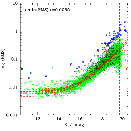
Figure 9: RMS versus magnitude plot for K-band data before recalibration. The black dots show all the data, the green crosses are objects classified as stars in the Source table and the blue squares are objects classified as variable. The red dashed vertical line is the expected magnitude limit for the intermediate stacks and the dashed curves are the best fit Strateva curves to the minimum RMS as a function of magnitude for each frame-set. Each line represents the empirical fit for the noise in a different pointing. The mean of the values aStrat, which represents the minimum RMS for a bright star is 0.0065 mag.

Fig 8 shows the histogram of the difference in zeropoints for intermediate stacks before and after recalibration. Recalibration of individual epochs makes a significant improvement in quality of the variability statistics and classification, as can be seen by comparing the “before” and “after” magnitude-RMS plots: Fig. 9 and Fig. 10. These plots show the RMS as a function of magnitude and are useful for diagnosing the noise properties of a frame or dataset and for finding variables. The red-dashed lines show the fit to the minimum RMS for each frame. Generally speaking there is good agreement between the stellar locus and the noise model, particularly at the faint end. The additional divergence at the bright end reflects the fewer data points. The noise flattens at the bright end when the random, “white” noise ceases to dominate and correlated “red” noise (see Irwin et al. 2007) becomes significant, as seen in Fig 9. In the better calibrated data, Fig 10, it is noticeable that the noise increases for the very brightest objects, which is not reflected in the noise model. This may be due to saturation effects. We have marked the objects classified as variables by blue boxes. In the recalibrated version, the typical minimum-RMS is $0.0047$ mag rather than $0.0065$ mag, meaning that the noise across all frames for a bright object is $\sim 0.002$ mag lower. If we are confident that $3\sigma-$detections are good, then we can detect variables with amplitudes of $0.013$ mag rather than $0.020$ mag. This is reflected in the larger number of blue squares in Fig 10.

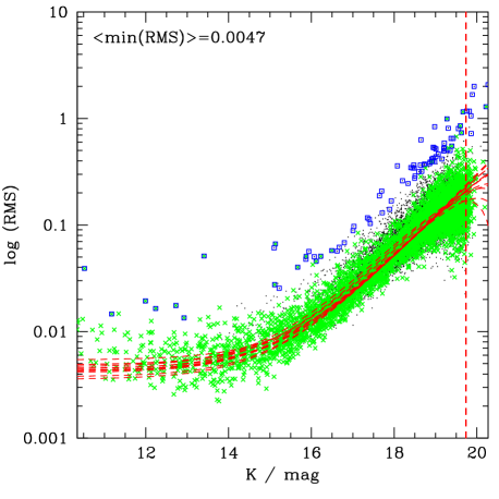
Figure 10: RMS versus magnitude plot for recalibrated K-band data. See Fig 9 for details. The mean of the values aStrat, which represents the minimum RMS for a bright star is 0.0047 mag.

This is just a very simple recalibration using a change in zeropoint. More complicated changes, fitting for spatial variations in both the astrometry and photometry are possible too. The recalibration only affects frames within a single pointing and we have not made any effort to recalibrate across pointings using overlaps, since the number of objects that can be used is much fewer. Only $\sim 3\%$ of the objects in a frame are in the overlaps, see Appendix B. Very good relative calibration can be achieved this way, but to get much better absolute calibration macro-stepping of the detectors is necessary to remove all instrumental effects. This involves observing the same large group of stars multiple times with different parts of the same detector and different detectors.

The astrometric error, sigDec ($\sigma_{\delta}$) is shown as a function of K-band magnitude in Fig 11 and shows a similar variation with magnitude as the photometric error. In the future, we will fit the magnitude-astrometric error in the same way as we fit the magnitude-photometric error in §4.3, see Fig 9.

Figure 11: Astrometric error versus magnitude plot in K-band for UKIDSS DXS data. The dots are galaxies and the squares are stars. For objects with $K<16$, the typical error is $0.015\arcsec$, and then gets larger for fainter objects.

5.2 Variable Objects

To find interesting variable objects, we select sources which are classed as variable, have mean magnitudes that are at least 3 magnitudes brighter than the expected magnitude limit in each band and not default and have more than 20 good observations in the K-band and more than 12 in the J-band. These last criteria are used since a typical DXS stack has 25 K epochs (see Fig 7) or 15 J epochs and we want to be close to the maximum to be able to see structure in the light curves. With this selection we found 40 objects. There are 3686 objects (variables and non-variables) which match these criteria apart from the variability classification. We looked through the light curves of all of these and selected the most interesting.

To use SQL to generate lightcurves for a specific source, see Appendix A or the SQL cookbook on the WSA interface. We give examples of a variety of variables in Fig 12 — 14. Fig 12 & 13 show two variables that are also classified as galaxies by the star-galaxy classifier and are also much redder than typical stars (in low extinction regions). The colours suggest that these are extragalactic objects, Active Galactic Nuclei (AGN), or heavily reddened stars, such as Asymptotic Giant Branch (AGB) stars (Guandalini & Busso 2008) which produce dust in their outer layers. These two objects are classified as extended sources in the deep images, but a slowly moving star may appear elliptical in a combination of images. We look at the distribution of the star-galaxy separation statistic classStat for the individual observations of these two objects. UDXSJ105639.43+575721.6 has $\overline{\rm classStat}_{K}=16.5\pm 4.7$ and $\overline{\rm classStat}_{J}=14.5\pm 2.5$. UDXSJ105644.55+572233.4 has $\overline{\rm classStat}_{K}=6.3\pm 1.6$ and $\overline{\rm classStat}_{J}=8.1\pm 2.0$. A point-source object is expected to have $-3.0\leq{\rm classStat}\leq 2.0$, so these two objects are certainly extended sources and are likely to be AGN. The first shows an undulating variation in both $J$ and $K$ bands, whereas the second shows are linear increase in brightness in $K$ over 700 days and a subsequent decrease in brightness in $J$. Fig 14 shows a star (based on colours and star-galaxy separation) that dims by more than 0.2 mag on several occasions in both $J$ and $K$. Follow up observations may prove this to be an eclipsing binary and determine the period.

Figure 12: Light curve for a variable galaxy, UDXS J105639.43+575721.6 Difference in magnitude around the median is plotted vs time in days from the first observation. Points with error bars show good observations. All the observations in this case were good. The statistics are calculated from the good observations only. The median magnitude of the observation is given. The light curve shows a clear minimum and maximum in the K-band, with an amplitude of $\sim 0.1$ mag. There is only the maximum in the J-band. There are not enough data to determine whether this is a periodic variable or not. This object is quite red: $(J-K)=1.27$ mag and has the profile of an extended source.

Figure 13: Light curve for a variable galaxy, UDXS J105644.55+572233.4. Points with error bars show good observations and circles without error bars show flagged observations. The light curve shows a linear increase in brightness in the K-band, with an increase of $\sim 0.2$ mag over $\sim 700$ days. In the J-band there is a decrease in brightness, but there are very few points taken at the same time. This object is quite red: $(J-K)=1.74$ mag and has the profile of an extended source.

Figure 14: Light curve for a variable star, UDXS J160650.11+544924.5. Points with error bars show good observations. The light curve is mainly flat in both bands but several dips of $\sim 0.2$ mag. More closely spaced observations could determine whether this is real (possibly an eclipsing binary) or not.

In addition to finding many real variables such as the example above, we also found some cases of poor calibration between adjacent overlapping frames, see Appendix B. To avoid regions with overlaps, it is best to set ${\bf priOrSec}=0$ in the Source table.

Figs 15 &  16 shows the magnitude-RMS plots for the whole of the UKIDSS-DXS Data Release 5 recalibrated intermediate data. Objects in the overlap regions have also been removed, apart from the 3 objects with interesting lightcurves shown in Figs 12 — 14. These three objects are in overlap regions, but the offsets across overlaps are minimal.

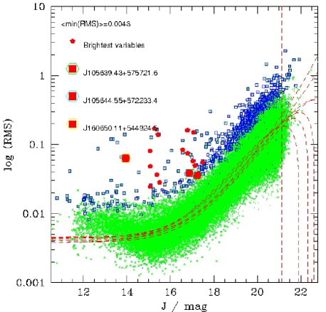
Figure 15: Magnitude versus RMS plot for $J$-band data. See Fig 9 for details. The mean of the values aStrat, which represents the minimum RMS for a bright star is 0.0043 mag. The small red pentagons are the brightest good variables described in Table 1 and the 3 large squares with coloured circles are the 3 objects of interest in Figs 12 —  14. There is a significant deviation in the RMS of the stellar population compared to the noise model for $J<14$ mag.

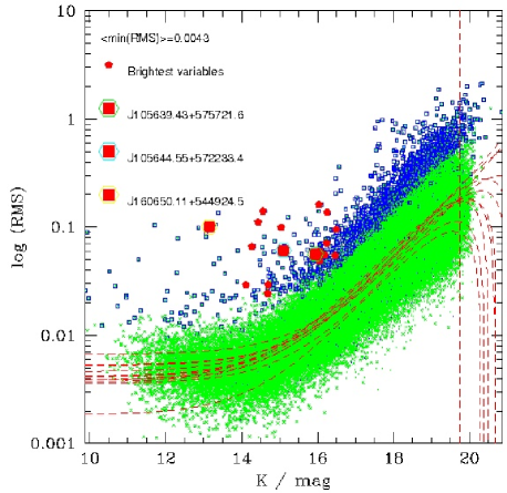
Figure 16: Magnitude versus RMS plot for $K$-band data. See Fig 15 for details. The mean of the values aStrat, which represents the minimum RMS for a bright star is 0.0043 mag.

Fig 15 shows a very noticeable increase in noise at the bright end ($J\leq 14$ mag), from the locus of the stellar population. There is not such a strong increase in the K-band. This noise has not been adequately modelled by the Strateva function and so the noise that goes into the variability calculations is under-estimated for $J<14$ mag, leading to excessive classifications of variable stars. This additional noise may be caused by a non-linearity or a saturation effect.

Table 1 lists the brightest variables in the DXS which are not in these overlap regions and which have $J\geq 14$ mag to avoid the effects of an incomplete noise model. We found 15 sources that matched our new criteria: classified as variable in both filters and having at least 10 good detections in each filter, out of a population of 11,957 sources that matched all the criteria apart from the variability criteria. These 15 objects are away from overlap regions and have magnitudes where the noise model is well fit and are the very best candidates for real variables.

These variables are plotted in Figs 15 &  16. Unfortunately most of the lightcurves are difficult to classify with only 15-20 points in each filter. To find and measure periodic variables, or eclipsing binaries, many more points would be needed. Some objects like supernovae can be usefully studied with this amount of data and these observations are very good for improving the calibration of the data. The objects in Table 1 can be followed up with more observations to properly determine their characteristics.

IAUName	Mag		RMS		Skew
(UDXSJ)	J	K	J	K	J	K
160509.10+542920.4	15.1	14.1	.024	.029	1.97	1.31
221809.44+002730.9	15.1	14.3	.048	.066	+2.59	+0.94
222052.62-000205.9	15.1	14.4	.080	.111	+0.55	+0.87
221706.04+002646.6	15.4	14.6	.140	.140	+1.83	+1.67
161206.50+543814.1	15.4	14.7	.036	.024	+1.62	+1.05
161244.51+541552.6	15.5	14.7	.028	.029	+0.05	+0.17
222139.61+004959.7	15.3	15.0	.170	.100	-0.01	+0.17
222049.30+003544.1	16.8	16.0	.074	.161	+2.35	+1.73
222106.51+004846.7	17.3	16.0	.036	.046	+2.31	-0.20
160519.04+542059.9	17.1	16.1	.049	.058	+1.93	+0.33
222215.25+010049.5	16.6	16.2	.084	.053	+0.75	+1.11
221953.96+001007.5	17.0	16.2	.057	.070	+3.29	+2.39
221714.27+003346.5	17.1	16.2	.150	.136	+1.41	+1.36
160504.88+543602.0	17.5	16.5	.054	.052	+1.52	+1.53
222117.36+010517.2	16.8	16.5	.161	.093	+0.09	+0.49

Table 1: Table of reliable variables, at least three magnitudes brighter than the per observation magnitude limit, in the DXS which are classified as variables in both filters and have more than 10 observations in each band and are not observed across an overlap. We have also removed any with $J\leq 14$ mag, since the noise properties of these are not well fit by the Strateva function at the bright end. These are mostly stars, but the entries marked in italics are classified as galaxies.

Table 2 is a table of the number of bright objects in each filter, as a function of object type (star, galaxy, noise, probable star) and variability (variable V, or non-variable NV), for objects outside the overlap regions. The proportion of stars that are classified as likely variables (classified using observations in that filter only: jvarClass or kvarClass) is $0.45\pm 0.05\%$ in the $J$-band ($14.0<J\leq 18.2$ mag) and $0.55\pm 0.05\%$ in the $K$-band ($11.5<K\leq 16.7$ mag). The proportion of galaxies classified as variable is $1.0\pm 0.1\%$ in the $J$-band and $1.5\pm 0.1\%$ in the $K$-band. While these limits are three magnitudes brighter than the limiting magnitude, the noise has already started increasing at $J\sim 16.5$ mag and $K\sim 15$ mag, so the lowest amplitude variables cannot be found. If we do limit the magnitudes to these brighter levels, we find $0.6\pm 0.1\%$ of stars are variable with $\Delta\,J\geq 0.015$ mag ($3\sigma$) and $1.7\pm 0.6\%$ of galaxies are variable. We find similar values in the $K$-band ($0.6\pm 0.1\%$ of stars and $2.3\pm 0.6\%$ of galaxies are variable with $\Delta\,K\geq 0.015$ mag). This estimate for the fraction of stellar variables is an underestimate, since variables with a much longer period than the total interval between observations will be excluded, and so will objects, like some eclipsing binaries, which have very little variation most of the time, but occasionally dip in brightness. If there are not enough observations to get several eclipses then these objects will also be excluded, as will objects that only vary sporadically. For galaxies, the noise model is not quite right, because all the photometry has been corrected for light loss outside the aperture, assuming that the objects are point spread functions. For stars and distant galaxies, this is the correct approach, but some nearby galaxies will not be corrected properly and the differences between the correction used and the true correction is an additional source of noise. This noise is not taken into account, and so the number of variable galaxies may be over-estimated.

Filter	Object	Var Type	Var Type	Number
	Type	(filter)	(overall)
J	Star	NV	NV	16252
J	Star	NV	V	12
J	Star	V	NV	47
J	Star	V	V	27
J	pStar	NV	NV	275
J	pStar	NV	V	4
J	pStar	V	NV	3
J	pStar	V	V	2
J	Galaxy	NV	NV	5577
J	Galaxy	NV	V	14
J	Galaxy	V	NV	50
J	Galaxy	V	V	10
J	Noise	NV	NV	14
K	Star	NV	NV	24164
K	Star	NV	V	8
K	Star	V	NV	24
K	Star	V	V	110
K	pStar	NV	NV	192
K	pStar	V	NV	3
K	pStar	V	V	5
K	Galaxy	NV	NV	12851
K	Galaxy	NV	V	2
K	Galaxy	V	NV	59
K	Galaxy	V	V	137
K	Noise	NV	NV	38
K	Noise	V	V	1

Table 2: Table of the classification of bright sources, at least 3 magnitudes brighter than the per observation magnitude limit, in the DXS after recalibration and fainter than the failure in the noise model. The sources must have at least 5 good observations to be included (since variables are only counted for objects with at least 5 good observations) and ${\bf priOrSec=0}$ to avoid bias from overlaps.

Next we look at the distribution of the variable stars versus non-variables. If we plot the ($J-K$) vs $K$ colour magnitude plot (Fig 17), we find three main groups of objects: 1) galaxies, with $(J-K)>1$; 2) stars with $0.6<(J-K)\leq 1$ and 3) stars with $(J-K)\leq 0.6$. We find that there are bright variables in each of these groups.

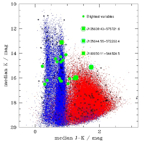
Figure 17: Colour-magnitude plot for UKIDSS-DXS data. The blue points are classified as stars and the red points are galaxies. The black squares are all variables. The good bright variables are plotted as green pentagons and the three interesting objects are marked by larger squares surrounded by a with different colour circle.

In Fig 18, we look at the distribution of variables in the intrinsic RMS versus skewness plane. Here we can see a definite bias towards positive skew for the brightest variables, and for variables in general, although the overall population of objects is quite symmetrical around a skew of zero.

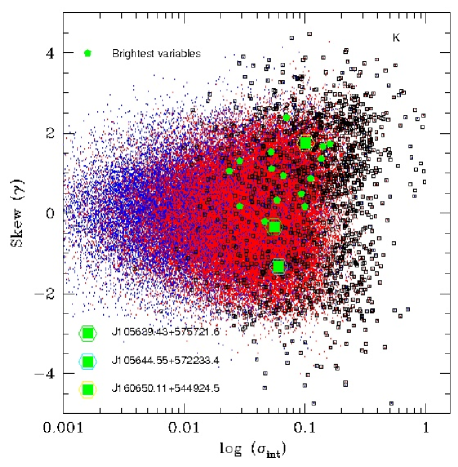
Figure 18: K-band intrinsic RMS vs skew for the UKIDSS-DXS. The blue points are classified as stars and the red points are galaxies. The black squares are all variables. The 20 good bright variables are plotted as green pentagons and the three interesting objects are marked by larger squares with a colour circle around.

6 Standard star data

While we have not yet released the WFCAM standard star data using this new archive model, we have produced some test data with our pipeline. We did the tests on one standard star field, the Serpens Cloud Core, chosen for the large number of individual observations $\sim 100$, the high density of stars, and because it includes three standard stars in the field, close to the cloud core. The standard star fields are 43 non-overlapping fields, although in some cases two pointings have been done around the same field to put the known standard onto different detectors. Since the Serpens Cloud Core is in a dense region of sky, liable to be confusion limited, we have only used seven epoch frames in each deep stack.

Since the observations are correlated, the same times are sampled in each light curve, which makes it much easier to distinguish which features are real variations. Fig 19 shows the histogram of the deviations in magnitude from the mean for three UKIRT faint standard stars Ser-EC51, Ser-EC68 and Ser-EC84 (Hawarden et al. 2001). These are all in the dense nebulosity of the centre of the cloud core. Ser-EC68 and Ser-EC84 show very little variation although EC84 is saturated in $H$, too bright for good detections in $K$ and too faint in $Z$. EC68 is also too faint in $Z$. The extinction in the cloud core means that very little radiation shorter in wavelength than $1\mu$m is visible. Ser-EC51 shows some large deviations from the median, particularly to fainter magnitudes. The light curve for this object shows some coherent variations 400 days after the first observation and 820 days after the first observation. Ser-EC51 should not be considered as a useful standard.

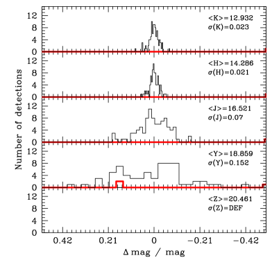
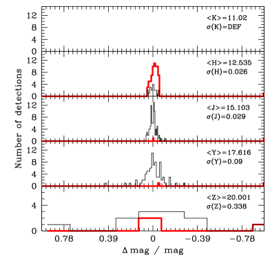
Figure 19: Histogram of difference in magnitude from the median for standard stars in the Serpens Cloud Core. Ser-EC51 (top), Ser-EC68 (middle) and Ser-EC84 bottom. The thin solid black histograms show the good observations and the thick solid red histograms show observations that we have flagged as having photometric problems. These stars are all very red, so there is very little Z-band flux and the K-band is saturated in the case of Ser-EC84.

Fig 20 shows the light curves of two other variable stars, chosen because of their interesting features. The top one shows a star that undulates slowly over a few hundred days, by 0.4 mag, before more rapidly dimming, by 1.3 mag, and rapidly brightening again. This may be an eclipsing binary. The lower object shows a longer term variation, with a rapid fading after 400 days, followed by a slow brightening. These were selected partly by using the Welch-Stetson statistics.

Figure 20: Light curve for two variable stars in the Serpens Cloud Core field. UCAL J182931.98+011842.5 (top) and UCAL J182955.19+011322.0 (bottom). Points with errorbars indicate good detections, circles indicate flagged detections and a dotted vertical line indicates a missing observation. The variations are highly correlated between each band.

The correlated band data is very useful as most real fluctuations are correlated (or anti-correlated) across many filters whereas most noise does not have a filter dependent correlation. Having so many more observations per source than the DXS also makes it easier to separate truly variable objects from ones with a few spurious measurements. Fig 21 shows that variable objects tend to have large absolute values of the Welch-Stetson statistic, as well as large values of the intrinsic RMS.

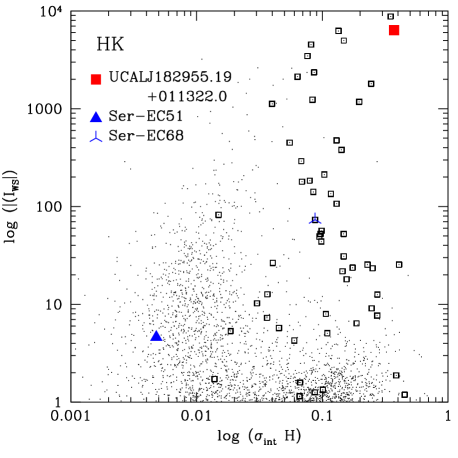
Figure 21: Plot of $H$-band intrinsic RMS vs absolute value of Welch-Stetson $|I_{WS,H,K}|$ for objects in the WFCAM Standard Star programme. Objects classified as variable have been marked by large squares. Three of the five objects with light curves are shown too. The other two, Ser-EC84 and UCALJ182931.98+011842.5 are saturated in $K$ and/or $H$ and so have a default value for $I_{WS,H,K}$. Ser-EC68 has low values of both parameters and is clearly non-variable, UCALJ182955.19+011322.0 has very large values of both and is clearly variable. Ser-EC51, is in between the two, but does show some signs of variation in the light curve.

7 VISTA-VIRCAM

We will apply the same data model to the VISTA Science Archive data. There are some features of VIRCAM which give additional problems.

• VIRCAM will usually have tiled images, with tiles made up of 6 observations, with the observations in the x-direction separated by $90\%$ of a detector width and those in the y-direction separated by $45\%$ of a detector width. These tiles are much larger than WFCAM detectors and are likely to have more calibration issues with half detector overlaps, and large distortion effects at the edges.

• The top and bottom of the tiles have a half detector width strip which only gets observed once, so cosmic ray and artifact removal is not possible. Some PIs may try to improve observing efficiency by stitching together these overlaps. Catalogued objects extracted from these stitched together overlaps will not have a single observation time, so they could not be used in any variability analysis and would have the additional problems of different noise and PSF and distortions in the original images.

• The focal plane can be independently rotated, so it is possible to have multiple rotations at the same pointing.

Much of the synoptic pipeline design has these issues in mind, but further work and tests with VIRCAM data will be necessary to fully solve them. As a result of the work on the synoptic pipeline that is presented in this paper, we have done away with the fixed number of filter passes used in shallow UKIDSS surveys and made all multi-epoch data sets synoptic (e.g. VISTA-VIKING). This gives the advantages of deep stacks, and internal recalibration, which surveys such as the UKIDSS-LAS will not enjoy. Additionally, this extra flexibility means that the schema does not have to be changed if an extra epoch is added in later.

7.1 Large Data Volumes

Frame sets from WFCAM are typically $0.05\deg^{2}$ (the area of one detector), but VISTA frame sets will be $\sim 1.5\deg^{2}$ (the area of a VISTA tile). Thus the number of objects per frame set will increase from a few thousand to more than 50,000 in a typical pointing and $\sim 1$million in a dense region of the Galactic plane. The UKIDSS UDS contains a single frame set of area $\sim 1\deg^{2}$ with 100,000 objects and has several hundred individual pointings. This has been successfully processed, so typical VISTA frame sets should pose few additional problems. Eventually, we will have to process the whole of the VVV: $\sim 10^{9}$ sources, with $\sim 100$ observations, producing a best match table with $\sim 10^{11}$ rows. The full processing of this must be done in $\leq 1$ month, if it is not going to significantly interfere with other archive processing and if we are going to be able to rerun the task. Our current processing speed is $\sim 2$hrs for the UDS field (using an older server). The VVV data set will be $\sim 3000\times$ larger. This problem is easy to parallelise, and factoring in Moore’s law (the main variability part of the VVV survey will not take place until year 3 of the surveys: 2012), a factor of $20\times$ the speed can be found without any optimisation. This gives a total time of $\sim 300$ hrs or $\sim 2$ weeks on four or more machines. Optimising the code so that it can run two or three times faster would allow the processing to be done on one or two machines over a sensible time scale.

8 Comparison with other public databases with multi-epoch observations

8.1 SDSS Stripe 82 database

The SDSS Stripe 82 is a 300 sq. deg. strip which has been observed 80 times in $u$, $g$, $r$, $i$, $z$ filters. The observations are taken in a drift scan mode with objects observed through each filter consecutively. The filter observations are therefore correlated within our criterion.

The Stripe 82 data has its own database (http://cas.sdss.org/stripe82/en), separate from other surveys. The database includes notes about how to search for all the detections of different objects. This uses the hierarchical triangular mesh identifier to search by position. This has the same drawbacks as the neighbour table approach in Paper 1:

• It is not possible to know whether there are missing observations, which are important in a lot of transient searches.

• In dense regions you will be contaminated by neighbouring objects, which having different magnitudes will make the objects appear variable.

However, there are also a couple of useful variability tables: Stetson, which is like a simplified Variability, containing a few photometric statistical values in each band and a continuous classification, and ProperMotions which contains the astrometric fit comparing the SDSS and USNO-B catalogues. These do not include any noise model as yet, although Sesar et al. (2007) have used one on the Stripe 82 data. Sesar et al. (2007) & Bramich et al. (2008) calculate many more statistics than are currently accessible through the main archive database.

Bramich et al. (2008) describe two useful tables, a Higher Level Catalogue (HLC) and a Light Motion Curve Catalogue (LMCC) which are similar to our Variability and SourceXSynopticSourceBestMatch, but these are only available as downloadable files which can be processed by an IDL programmes. It is not possible to search through them using the SDSS query tools and then to match up with external catalogues.

While much work has been done on measuring variability in the SDSS Stripe 82 data, this work is in several separate publications and very little of this is currently available in the main SQL query tool, so it is not easy for users to search on variability statistics. In contrast we have designed our multi-epoch pipeline and archive together, so users can access all our parameters and do more detailed searches on a wide range of different types of variables.

8.2 NSVS public database

The NSVS public database (Woźniak et al. 2004a) contains six tables. These are Field, Frame, Object, Synonym, Observation and Orphan. The NSVS observations were all taken in a single, wide optical filter, which is closest to the Johnson R filter of all the standard filters. The main variability table, Object, contains $\sim 2\times 10^{7}$ sources and is similar in scope to our Variability table. It contains an ID, the median and standard deviation of the right ascension and declination, the median of the magnitude and median and standard deviation of the differences in magnitude of the from “good” points, the number of points, number of good points and number of points with a certain flag type as well as the flags associated with the object. The Observation table is similar to a combination of our best match and Detection tables, listing all the individual observations linked to each object. It includes the position, magnitude, magnitude error and flags only. The Synonym table is equivalent to our SourceNeighbours table linking identical objects to each other. The Frame table is similar to our Multiframe table, describing each observation and the Field table is similar to RequiredStack describing the pointing information. The Orphan table is very interesting: it contains bright objects that aren’t linked to any object. These could be fast moving objects (solar-system objects) that have moved too much between observations to be linked to each other or objects that are very faint but flare up, only to be seen on a few frames.

The NSVS public database is similar to ours and light-curves can be easily selected from it, like the WSA, but it lacks any modelling of the noise or any attempt at classifying variables so it is much more difficult to reduce the number of objects that you are searching through to a manageable number. This is left for the user to do. However, searching thousands of light-curves is no simple task and many users will be repeating the same type of analysis: checking the noise properties and eliminating objects that are too close to the noise limit, so it would be good to have these useful quantities in the database to search on.

A follow up paper (Woźniak et al. 2004b), describes how to use the database to select candidate red variables, using light curve information from Observation and aggregate data from Object.

9 Summary and Future Work

We have designed, implemented and released a dynamic archive for analysing time series data containing both astrometric and photometric variations which works on a wide variety of data sets observed by either the UKIRT-WFCAM or VISTA-VIRCAM instruments. The design of the archive can be used (with small modifications) on any astronomical data from pointed observations. It is designed so that the data can continue to be updated and improved, and additional refinements included without repeating every step again. We have included measurements of the noise properties that are essential for determining whether the object is variable and properties of the observation sequence, such as the typical observation interval.

This paper describes the design of the synoptic pipeline in the WFCAM Science Archive and is useful for the design of future archives for synoptic surveys such as Pan-STARRS and LSST. This paper is also a useful handbook for users of the WSA and VSA, so that they can use the facilities to do useful science with variable objects.

The archive of synoptic data is also useful for global calibration of UKIDSS and VISTA data, since the data has now been more efficiently matched and non-variables can be selected. Some spatial variations within the detectors have been seen in synoptic data. New standard stars can be selected from the data and previous standards tested more thoroughly.

We have made it possible, using these archive tools, to rapidly reduce a massive database of millions or billions of sources into a few tens of potentially interesting variable objects. The synoptic pipeline is still being developed and we expect to add in many of the following features in the future:

• Improved calibration

  — a spatially dependent relative photometric and astrometric recalibration. This will be more sophisticated than the simple zeropoint shift at present.

  — calibrate across the overlaps to correct for the discontinuity in calibration across overlaps.

• Improved noise model

  — an additional component that takes into account the increase in astrometric noise at the bright end.

  — fitting astrometric errors as a function of magnitude.

  — moving from an empirical fit to a model dependent on filter, exposure time and sky brightness, so that sets of observations with different exposure times can be weighted correctly. This will involve a lot of careful analysis of the noise in different frames, across many programmes first.

  — estimation of effects of red (correlated) noise.

• Moving objects

  — fitting the astrometric data for proper motions (and parallax).

  — a table of fast moving objects: i.e. objects that are too far apart to be stacked together in deep stacks, but are good detections at individual epochs.

• List-driven photometry. This gives un-biased statistics for faint objects and could improve the RMS for non-moving sources by removing errors caused by inconsistent centring of the object.

• Difference imaging. This may be necessary to find variables in very crowded regions.

• More sophisticated cadence statistics. The median cadence gives a useful idea of the typical interval between observations, but the mode (or modes in a multi-peaked distribution) would be more useful. The minimum and maximum give the range of time between observations, but these can be skewed by an unusual observation, so taking the 10th percentile and 90th percentile of time between observations would give a more robust measure of the range of observations.

• Additional photometric statistics, such as the fraction of points more than 3 standard-deviations from the mean magnitude, the kurtosis of the $\Delta$mag distribution and statistics on the star-galaxy separation. The first two of these constrain the properties of the light-curve and the last gives better morphological information.

• Fourier analysis to get periodicities and the light curve shape. This could be part of our data analysis services, so users request particular objects, rather than a wholesale processing of all data.

• More sophisticated variable classification and classification of different types of variable. This will use more of the photometric statistics such as the skewness, the Welch-Stetson statistic as well as astrometric information to produce a wider range of classes that will increasingly help users to isolate a group of objects that interest them, such as eclipsing binaries, periodic variables, high proper motion stars, cataclysmic variables.

We have started investigating and planning some of the improvements, and will continue to do so as WFCAM and VISTA continue operations. All changes will be documented on the archive websites.

9.1 Moving Objects

One of the future improvements is to add a proper-motion calculation into the astrometric statistics. The astrometric part of the pipeline has not progressed far enough for it to be easy to find moving objects, such as the high proper-motion star UDXS J222223.70+000324.3, see Fig 22. This was found through a comparison with 2MASS instead. This object has $\mu_{\alpha}\sim 0.23\arcsec$year^-1 and $\mu_{\delta}\sim 0.13\arcsec$year^-1. The DXS observations fall into two batches (see Fig 22a), and only the later smaller batch are linked to the source through the best-match table. The other detections are too far apart and so this source has many missing observations even though it is bright ($J=12.6$ mag, $K=11.8$ mag). A faster moving object, and one where the observations are more evenly sampled may be missed in the deep images altogether, because the stacking algorithm uses median clipping to remove false detections.

The object can be tracked back through the neighbour table to 2MASS, and through the Supercosmos Science Archive (Hambly et al. 2004) to plates taken over 20 years ago, see Fig 22b.

Figure 22: Time varying position of high proper-motion star UDXS J222223.70+000324.3. The top plot (a) shows the UKIDSS-DXS observations, which are clustered around two epochs. The dots with errorbars are the J-band observations and the crosses with errorbars are the K-band ones. The lower plot (b) shows the same star, but older observations from 2MASS and the Super-Cosmos Science Archive (SSA) have been added in. It has a very clear constant proper motion. In both plots RA=RA$-330$ deg for presentation purposes.

This is a particularly high proper motion star, and most of those that users are interested in will be moving much more slowly. However, it is a useful example of the problems that are faced when automating a search for moving objects. Because of examples like this, we increased the maximum distance in the SourceXDetection neighbour table for UKIDSS-DR5 from $1\arcsec$ to $10\arcsec$.

In many cases, if the complete data set is taken over a very short time — much less than a year — very few stars have moved enough to be detectable. Therefore, in later variants of the pipeline, it would be sensible to incorporate a test which calculates the minimum proper motion rate,

$$\mu_{\rm min}=\frac{\sigma_{\rm astrm}}{T_{\rm max}},$$ (11)

where $T_{\rm max}$ is the maximum observation time between observations for any source in a dataset and $\sigma_{\rm astrm}$ is the typical astrometric error for bright sources and $\mu_{\rm min}$ is the minimum proper motion rate. If $\mu_{\rm min}$ is less than a rate which will find many scientifically interesting candidates ($\mu\sim 0.05\arcsec\,$year^-1), then the proper motion will be evaluated for all objects in the dataset, otherwise no proper motions will be calculated. The error in the DXS astrometry is $\sigma_{\rm astrm}\sim 0.015\arcsec$, see Fig 11, and the period of observations in any pointing is $T_{\rm max}\sim 2$ years, giving a minimum proper motion of $\mu_{\rm min}\sim 75$mas year^-1.

The parallax calculation may be invoked similarly.

Solar system objects have much larger motions, so running the proper motion code on shorter timescale datasets could pick out these objects. On long timescale datasets, these will show up as detections unmatched to any source, since the stacking clips out detections that are not repeated at the same position in other frames that contribute to a deep stack.

9.2 Improved test for missing objects

In Fig 4 we showed the current method of testing whether a source should have been observed. Fig 23 shows that this method will be very inefficient on VSA rectangular tiles: the area between the two radii is extremely large and so a lot of sources must undergo the slow step 2 of determining whether the object was in the pointing and should have been observed. A more efficient routine needs to reduce the number of objects for which step 2 is necessary for determination. The modified step 1 must still be very efficient. Using a simple RA and DEC selection is no good, because VISTA tiles can be rotated. Instead we use a method in which the distance from each of the four corners is calculated, and from those calculations, the areas of the four triangles from each edge of the tile to the source are calculated. If the areas of the four triangles is equal to the area of the rectangle, then the source is within the tile, else it is outside. The area of the rectangle and triangles will be somewhat distorted by the image projection and so the area calculated for the triangles may not be equal to the area of the rectangle, even when it is inside the rectangle. Some uncertainty may exist until the area of the triangles is quite a bit larger than the area of the rectangle. This may mean increasing the area that the more careful second stage is used in, but this area should still be significantly smaller than the area between the circles.

Figure 23: The difficulties of finding whether an object should have been observed on a VIRCAM tile. A tile at orientated at 34 degrees is shown as an example. For rectangular tiles, the radius method used in Fig 4 is very inefficient. Calculating distances from the four corners and the areas of the triangles formed by the object and the corners is slower than the radius method, but much faster than calculating the x and y position. The area of the triangles formed by the red dotted lines and the edges of the tile is the same as the area of the tile. The area of the triangles formed by the blue dotted lines and the edges is greater than the area of the tile. Objects inside and outside the tile can easily be distinguished. Only a very small number of objects very close to the edge will need to have their x and y positions calculated.

An alternative method is to use the half-space method (Budavári et al. 2007). In this method, each edge of the frame is an edge on a plane that intersects the sphere of the sky. The plane is represent by the orthonormal vector and an offset from the centre of the sphere. It is easy to tell which side of the plane a point is through its dot-product. Repeating this for each edge of the frame tells you whether the object is in or out of the frame. The plane can be calculated using cross-products of the coordinates. These only have to be done once for each frame, and the dot-products that need to be calculated four times for each point are computationally very simple and quick. This also has the advantage that it is clear-cut whether an object is either side of each line. We will test these two methods to see which gives the best performance.

10 Acknowledgements

NJGC would like to thank Nicolas Lodieu and Richard Jameson for their inspiration at the 2007 UKIDSS meeting in Munich. NJGC would also like to thank Leslie Hebb for useful early discussions on analysis of variables and Tamás Budavári for more recent discussions on footprints. We would like to thank the anonymous referee for useful suggestions and a quick report.

Financial resources for VISTA/WFCAM Science Archive development were provided by the UK Science and Technology Facilities Council (STFC; formerly the Particle Physics and Astronomy Research Council) via e–Science project funding for the VISTA Data Flow System and Rolling Grants. Operations resources, including provision for hardware, are provided in the main by the STFC, but we would also like to acknowledge significant contributions to hardware funding from University of Edinburgh sources.

Appendix A Example Queries

Throughout these queries xxx replaces the programme name: e.g. dxs, uds, cal for the UKIDSS-DXS, UKIDSS-UDS and WFCAM standard star observation programmes respectively. To select all reliable variable stars which are 3 magnitudes brighter than the expected magnitude limit in the K-band.

SELECT v.sourceID,v.kMeanMag,v.kMagRms
FROM   xxxSource AS s,xxxVariability AS v,
       xxxVarFrameSetInfo AS i
WHERE  s.sourceID=v.sourceID AND
       v.frameSetID=i.frameSetID AND
       s.mergedClass=-1 AND v.variableClass=1
       AND v.kMeanMag<(i.kexpML-3.) AND v.kMeanMag>0.
       AND s.priOrSec=0

The first two lines of the “WHERE” statement links the 3 tables used in this SQL statement. If these tables are not properly linked then you have what is called a Cartesian join: every line in one is joined to every line in the others, which takes a long time to return and does not return what is wanted. It is best to link tables through the primary key (see the Schema Browser for the primary key and indices for each table), if possible, since the primary key is unique and indexed, making a particularly quick return. The Source and Variability tables have sourceID as the primary key, and VarFrameSetInfo has frameSetID as the primary key. The other selections are straight-forward: ${\bf s.mergedClass}=-1$ selects objects classified as stars, ${\bf v.variableClass}=1$ selects objects classified as variable, ${\bf s.priOrSec}=0$ selects objects that are away from overlaps. ${\bf v.kMeanMag}<({\bf i.kexpML}-3.)$ selects objects which are 3 magnitudes brighter than the expected magnitude limit for that frame. The ${\bf kMeanMag}>0$ removes any objects with default magnitudes. Additional terms for the number of good matches, the skewness, the median interval, or the RMS can also be applied as necessary.

To select a light curve from the archive, use the following, if the band passes are uncorrelated (the best match table is a SourceXDetectionBestMatch):

SELECT m.mjdObs,d.aperMag3,d.aperMag3Err,
       d.ppErrBits,x.flag
FROM   xxxSourceXDetectionBestMatch AS x,
       xxxDetection AS d,Multiframe AS m
WHERE  x.sourceID=NNN AND x.multiframeID=
       d.multiframeID AND x.extNum=d.extNum AND
       x.seqNum=d.seqNum AND x.multiframeID=
       m.multiframeID AND d.filterID=5
ORDER BY m.mjdObs

This selects the full light curve for sourceID=NNN. Both the SourceXDetectionBestMatch and Detection tables contain objects from all filters used in the programme, so it is important to have a selection on filterID. The time term is a modified Julian date, which is found in the Multiframe table. Ordering by mjdObs puts the results in time order. The last 2 output terms are useful for determining how good the light curve is. The ppErrBits flag tells the user if the object has been flagged for potential poor photometry. The best match table flag is also useful: if flag=1 then the object has been matched to two sources, suggesting either motion or deblending; if flag=2 then the lack of detection is probably due to the object being within a dither offset of the edge of the frame, and not a source that has taken a drastic dip in brightness.

If the band passes are correlated, so that a SynopticSource table is produced, then the following produces a similar light curve:

SELECT ml.meanMjdObs,e.kaperMag3,e.kaperMag3Err
       e.kppErrBits,x.flag
FROM   xxxSourceXSynopticSourceBestMatch AS x,
       xxxSynopticSource AS e,
       xxxSynopticMergeLog AS ml
WHERE  x.sourceID=NNN AND x.synFrameSetID=
       e.synFrameSetID AND x.synSeqNum=e.synSeqNum
       AND e.synFrameSetID=ml.synFrameSetID
ORDER BY ml.meanMjdObs

For correlated bandpasses, light curves can be produced for several filters together:

SELECT ml.meanMjdObs,e.japerMag3,e.japerMag3Err,
       e.jppErrBits,e.kaperMag3,e.kaperMag3Err,
       e.kppErrBits,x.flag
FROM   xxxSourceXSynopticSourceBestMatch AS x,
       xxxSynopticSource AS e,
       xxxSynopticMergeLog AS ml
WHERE  x.sourceID=NNNNNNNNNN AND x.synFrameSetID=
       e.synFrameSetID AND x.synSeqNum=e.synSeqNum
       AND e.synFrameSetID=ml.synFrameSetID
ORDER BY ml.meanMjdObs

Appendix B Overlaps

While there are many real variables, there are also a great many which are false. Consider the object in Fig 24. This object seems to have two separate light-curves. Unfortunately this is not a high frequency periodic variable, but indicates that there are still some spatial systematics that have not been removed in the calibration (Hodgkin et al. 2009). The variation is strongly correlated with position on the field, since this object is in a region overlapping two pointings.

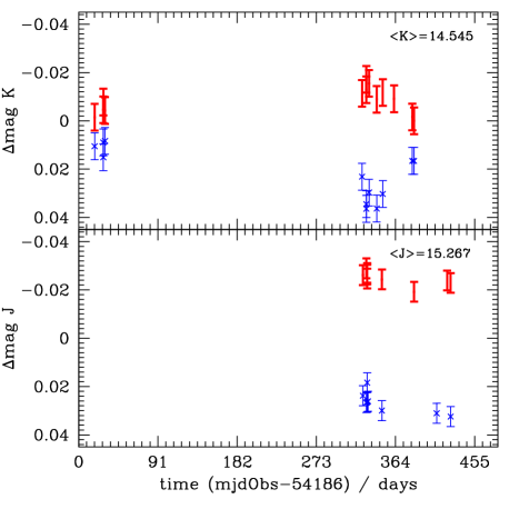
Figure 24: Light curve for object, UDXS J105553.80+583930.7. The points that have ${\bf extNum}=4$ and $y<500.$ are marked by points with thick error bars and those with ${\bf extNum=4}$ and $y>3500.$ are marked by crosses with thin error bars. It is immediately apparent that the majority of the variation is dependent on the position on the field, and is not intrinsic.

B.1 Describing overlaps

The overlaps between different pointings can be complicated, due to WFCAM having 4 non-buttable detectors. With the typical overlapping there are 16 possibilities (not counting ones across a diagonal from each other). We found all these 16 possibilities (one along each side of each of the 4 detectors), see Fig 25, with an additional 2 arrangements where the pointings were not arranged as expected, see Fig 26.

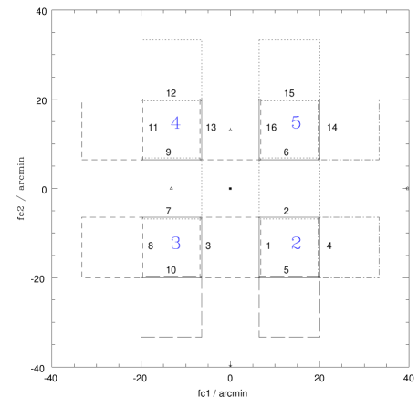
Figure 25: Typical arrangements of pointings in the DXS (and most WFCAM datasets). The black solid lines show the pointing in question. The dot, dashed, long-dashed and dot-dashed lines show the neighbouring pointings with overlaps along a detector edge. The extension numbers are given in large blue numerals. Each overlap is numbered by a smaller black number. These numbers are the indices in Table 3.

Figure 26: Non-typical arrangements of overlaps in the DXS. These occurred when good guide stars were not present at the original pointing positions and so the pointings were moved by a few arc-minutes. The solid line shows the pointing and the dotted line shows the neighbouring pointing. ${\it 19}$ is an overlap where there were no J or K sources (with at least 20 good observations).

To describe each of these overlaps, we need a consistent set of labels. We use the following descriptor: X1_X2_N, where X1 is the extNum of the first frame, X2 is the extNum of the second frame and N is a number describing which borders of each detector are used. The extNums do not uniquely describe an overlap by themselves as can be seen in Fig 25. A further complication is that the x and y axes rotate by 90 degrees from detector to detector (see Dye et al. 2006, Fig 1). A typical overlap lies along the full length of the x- or y- axis and the width of the overlap is typically $3\%$ of the width of the detector, so the distribution of the sources between any two frame sets can specify which overlap it is in. We find frame set pairs by looking for sources which are in two different deep stacks, i.e. priOrSec$>0$ and then using the dxsSourceNeighbours table and Source table to find the frame sets. We checked though all overlaps (except at corners where the number of sources is minimal). In each overlap, we calculate the mean and standard deviation of the x-coordinate and the mean and standard deviation of the y-coordinate for both frames. If the overlap is long along the y-axis and narrow along the x-axis and close to $x=0$ then $<x>\sim 0.5w$, $\sigma(x)\sim 0.25w$, $<y>\sim 0.5l$, $<y>\sim 0.25l$ ($w$ is the width of the overlap, typically $0.03$ of the detector size $l$). We assign one of three values to each of the four coordinates (x1, y1, x2, y2). If the mean is close to the detector mid-point, then the value is 0, if it is close to 0, then the value is 1, and if it is close to the maximum, then the value is 2. We also make sure the standard deviation is high in the first case and low in the later cases. The descriptor $N$ is therefore:

$$N=\sum_{i}a_{i}3^{4-i}$$ (12)

where $a_{i}$ is the value of the $i^{th}$ coordinate. So the overlap of extension 2, along the y-axis, at $x\sim 0$ with extension 5, along the x-axis at $y\sim 4000$ has $a_{0}=1$ ($<x1>$: minimum), $a_{1}=0$ ($<y1>$: midpoint), $a_{2}=0$ ($<x2>$: midpoint), $a_{3}=2$ ($<y2>$: maximum). The overlap is therefore 2_5_29. Table 3 describes all the overlaps in Figs 25 & 26. These overlaps all have mirror images (e.g. 2_2_11$=$2_2_19 and 2_5_55$=$5_2_15. We have always ordered them with the lowest extension number first.

Index	ID	No.		$\Delta\,$mag
		J	K	J	K
1	2_2_11	13	13	$-0.001\pm 0.003$	$0.000\pm 0.005$
2	2_2_33	25	32	${\bf 0.011\pm 0.002}$	$0.009\pm 0.003$
3	2_3_15	11	16	$-0.005\pm 0.006$	$0.006\pm 0.003$
4	2_3_21	24	62	$0.001\pm 0.007$	$-0.003\pm 0.002$
5	2_5_29	26	29	$0.001\pm 0.003$	$-0.007\pm 0.002$
6	2_5_55	58	45	$0.004\pm 0.001$	${\bf 0.010\pm 0.002}$
7	3_3_11	26	33	$-0.009\pm 0.002$	${\bf-0.017\pm 0.002}$
8	3_3_33	21	28	${\bf 0.017\pm 0.003}$	${\bf 0.025\pm 0.003}$
9	3_4_15	44	62	$0.007\pm 0.002$	$0.001\pm 0.001$
10	3_4_21	11	23	${\bf 0.017\pm 0.003}$	${\bf-0.011\pm 0.003}$
11	4_4_11	17	32	${\bf-0.023\pm 0.004}$	${\bf-0.034\pm 0.003}$
12	4_4_33	29	39	$0.007\pm 0.002$	${\bf 0.013\pm 0.002}$
13	4_5_15	10	16	$-0.006\pm 0.005$	$-0.003\pm 0.002$
14	4_5_21	11	63	$0.001\pm 0.004$	$0.003\pm 0.003$
15	5_5_11	35	32	$-0.005\pm 0.002$	${\bf-0.013\pm 0.003}$
16	5_5_33	30	21	$-0.001\pm 0.002$	$0.007\pm 0.004$
17	2_5_24	4	2	${\bf-0.037\pm 0.007}$	$0.003\pm 0.009$
18	3_4_56	4	5	${\bf-0.029\pm 0.005}$	${\bf-0.045\pm 0.006}$
19	2_4_10	0	0	$---$	$---$

Table 3: Table of the overlaps in the DXS. This gives the number of J and K sources in the overlap regions, with at least 20 good observations per source. $\Delta\,J$ and $\Delta\,K$ represent the typical difference in magnitude across the offset. The bold numbers are offsets with $\Delta\,m>0.01$ mag

To get from $N$ to the borders, simply convert N into a 4-digit base 3 number (e.g. 11=0102). The first 2 digits tell you which is the border for the first frame (01: along the x-axis with $y\sim\,y_{min}$) and the last two digits tell you which is the border for the second frame: (02: along the x-axis with $y\sim\,y_{max}$).

B.2 Offsets

To calculate the offsets between overlaps, we assume that each different type of overlap is affected in the same way, wherever in the survey it is, i.e. a 2_2_11 overlap between two observations in the ELIAS N1 region of the UKIDSS-DXS will have the same offset as another 2_2_11 overlap between two other observations in the ELIAS N1 region or a 2_2_11 overlap in the Lockman Hole region. Finally we select objects that have a magnitude $(m_{limit}-7.)<m<(m_{limit}-3.)$ where $m_{limit}$ is the J or K-band limit in the VarFrameSetInfo table, see §4.3. The brighter limit should reduce effects of saturation and the fainter limit should remove very noisy objects.

We calculate $\Delta\,mag$ very simply by finding the $3\sigma-$clipped mean magnitude of each source from observations on one side of the overlap and subtracting the equivalent value on the other side. Some of these sources vary in time and have different numbers of observations on each side, corresponding to when the observations were taken. However, these variations are different for each source and just add some addition random error if there are enough sources in each overlap.

The offsets for each overlap are shown in Table 3.

B.2.1 Variations with position and magnitude.

In each overlap region we have looked for variation with position or magnitude. We look at the coordinate along the primary direction of the first extension (i.e. along the side of the detector) We have plotted a subset of the overlaps showing some with large offsets, some with small offsets in Figs 27 - Fig 30. The full set of plots can be found at http://surveys.roe.ac.uk:8080/wsa/Overlaps/overlaps.html. While we find some linear trends with position, there seems to be no noticeable variation with magnitude over the 4 magnitudes in question. This suggests that the problem is not due to saturation or non-linearities in the photometric solution, but is due to a spatial variations across the focal plane which have not yet been eliminated.

Figure 27: Relative photometry of the sources on either side of the K-band 2_2_11 overlap. The lower plot shows the variation with the position, and the upper plot shows variation with magnitude. The red solid line gives the mean offset and the red dashed lines give the $3-sigma$ deviation from this offset. The blue dotted line gives the best fit linear variation with position. This overlap shows no significant offset and no significant trend with magnitude or position.

Figure 28: Relative photometry of the sources on either side of the J-band 2_2_33 overlap. See Fig 27 for details. This overlap shows a significant offset $0.011\pm 0.002$ mag. There is no significant trend with magnitude or position.

Figure 29: Relative photometry of the sources on either side of the K-band 3_4_15 overlap. See Fig 27 for details. This overlap between two different detectors shows no significant offset or trends.

Figure 30: Relative photometry of the sources on either side of the J-band 4_4_11 overlap. See Fig 27 for details. There is a significant offset $-0.023\pm 0.004$ and a strong trend with position. Again there is no trend with magnitude.

B.3 Correcting lightcurves

Above, we have done a careful analysis of the overlaps and conclude that the offsets across most overlap regions are low level $<0.01$ mag (as expected from Hodgkin et al. 2009), but in a few cases, particularly between extension number 4 on one frame and extension number 4 on the other, along the x-axis, can be several hundredths of a magnitude — almost 10 times the expected value (see Table 3). There is no magnitude dependence, but there is a positional dependence along some of the overlaps, so this is not an effect of saturation. Fig 31a shows the effect of correcting the light curve in Fig 24 with the average offset measured along the overlap. Some of the difference in the lightcurves is removed. Fig 31b shows the effect of correcting with a positional dependent offset, and in this case most of the difference is removed.

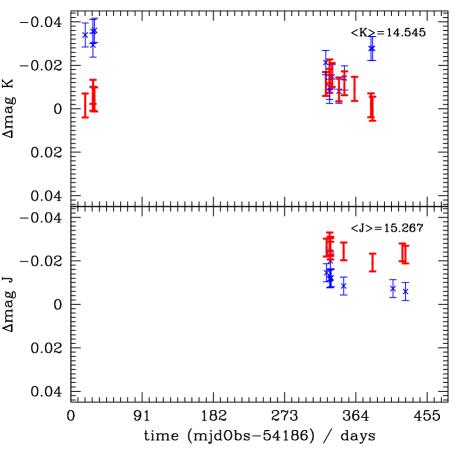
Figure 31: Light curve for object, UDXS J105553.80+583930.7. Same labelling as for Fig 24, except that in the upper plot (a), the points having $y>3500.$ (crosses with thin error bars) have been corrected by a simple offset for the whole overlap, and in the lower plot (b), these points have been corrected using a linear fit to position. The points having $y<500.$ have not been altered in either case. With this second correction most of the difference is removed.

References

- Alcock et al. (2000) Alcock C., Allsman R. A., Alves D. R., et al., 2000, ApJ, 542, 281
- Bertin & Arnouts (1996) Bertin E., Arnouts S., 1996, A&AS, 117, 393
- Bessel (1838) Bessel F. W., 1838, MNRAS, 4, 152
- Brahe & Kepler (1602) Brahe T., Kepler J., 1602, Tychonis Brahe Astronomiae instauratae progymnasmata : quorum haec prima pars de restitutione motuum SOLIS et lunae stellarumque inerrantium tractat, et praeterea de admiranda nova stella anno 1572 exorta luculenter agit., Brahe T., Kepler J., eds.
- Bramich et al. (2008) Bramich D. M., Vidrih S., Wyrzykowski L., et. al., 2008, MNRAS, 386, 887
- Budavári et al. (2007) Budavári T., Dobos L., Szalay A. S., Greene G., Gray J., Rots A. H., 2007, in Astronomical Society of the Pacific Conference Series, Vol. 376, Astronomical Data Analysis Software and Systems XVI, Shaw R. A., Hill F., Bell D. J., eds., pp. 559–+
- Collins et al. (2009) Collins R., Cross N., Sutorius E., Read M., Hambly N., 2009, in Astronomical Society of the Pacific Conference Series, Vol. in press, Astronomical Data Analysis Software and Systems XVIII, Bohlender D. A., Durand D., Dowler P., eds.
- Cross et al. (2007) Cross N., Hambly N., Collins R., Bryant J., Mann B., Read M., Sutorius E., Williams P., 2007, in Astronomical Society of the Pacific Conference Series, Vol. 376, Astronomical Data Analysis Software and Systems XVI, Shaw R. A., Hill F., Bell D. J., eds., p. 54
- de Wit et al. (2006) de Wit W. J., Lamers H. J. G. L. M., Marquette J. B., Beaulieu J. P., 2006, A&A, 456, 1027
- Djorgovski et al. (2008) Djorgovski S. G., Baltay C., Mahabal A. A., Drake A. J., Williams R., Rabinowitz D., Graham M. J., Donalek C., et al., 2008, Astronomische Nachrichten, 329, 263
- Drake et al. (2009) Drake A. J., Djorgovski S. G., Mahabal A., Beshore E., Larson S., Graham M. J., Williams R., Christensen E., et al., 2009, APJ, 696, 870
- Dye et al. (2006) Dye S., Warren S. J., Hambly N. C., et al., 2006, MNRAS, 372, 1227
- Emerson et al. (2004) Emerson J. P., Sutherland W. J., McPherson A. M., Craig S. C., Dalton G. B., Ward A. K., 2004, The Messenger, 117, 27
- Goodricke (1783) Goodricke J., 1783, Royal Society of London Philosophical Transactions Series I, 73, 474
- Graham et al. (2004) Graham M. J., Williams R., Djorgovski S. G., Mahabal A., Baltay C., Rabinowitz D., Bauer A., Snyder J., et al., 2004, in Astronomical Society of the Pacific Conference Series, Vol. 314, Astronomical Data Analysis Software and Systems (ADASS) XIII, Ochsenbein F., Allen M. G., Egret D., eds., p. 14
- Guandalini & Busso (2008) Guandalini R., Busso M., 2008, A&A, 488, 675
- Hambly et al. (2004) Hambly N., Read M., Mann R., Sutorius E., Bond I., MacGillivray H., Williams P., Lawrence A., 2004, in Astronomical Society of the Pacific Conference Series, Vol. 314, Astronomical Data Analysis Software and Systems (ADASS) XIII, Ochsenbein F., Allen M. G., Egret D., eds., p. 137
- Hambly et al. (2008) Hambly N. C., Collins R. S., Cross N. J. G., et al., 2008, MNRAS, 384, 637
- Handler (2003) Handler G., 2003, Baltic Astronomy, 12, 243
- Hawarden et al. (2001) Hawarden T. G., Leggett S. K., Letawsky M. B., Ballantyne D. R., Casali M. M., 2001, MNRAS, 325, 563
- Hawkins (2000) Hawkins M. R. S., 2000, A&AS, 143, 465
- Hodgkin et al. (2009) Hodgkin S. T., Irwin M. J., Hewett P. C., Warren S. J., 2009, MNRAS, 394, 675
- Hu et al. (2007) Hu S.-M., Bi X.-W., Zheng Y.-G., Mao W.-M., 2007, in Astronomical Society of the Pacific Conference Series, Vol. 373, The Central Engine of Active Galactic Nuclei, Ho L. C., Wang J.-W., eds., p. 205
- Huber et al. (2006) Huber M. E., Everett M. E., Howell S. B., 2006, AJ, 132, 633
- Irwin et al. (2007) Irwin J., Irwin M., Aigrain S., Hodgkin S., Hebb L., Moraux E., 2007, MNRAS, 375, 1449
- Ivezić et al. (2008) Ivezić Ž., Axelrod T., Becker A. C., et al., 2008, in American Institute of Physics Conference Series, Vol. 1082, American Institute of Physics Conference Series, pp. 359–365
- Kaiser (2007) Kaiser N., 2007, in Advanced Maui Optical and Space Surveillance Technologies Conference
- Kholopov et al. (1998) Kholopov P. N., Samus N. N., Frolov M. S., et al., 1998, in Combined General Catalogue of Variable Stars, 4.1 Ed (II/214A). (1998), p. 0
- Kochanek et al. (2008) Kochanek C. S., Beacom J. F., Kistler M. D., Prieto J. L., Stanek K. Z., Thompson T. A., Yüksel H., 2008, ApJ, 684, 1336
- Law et al. (2009) Law N. M., Kulkarni S., Ofek E., Quimby R., Kasliwal M., Palomar Transient Factory Collaboration, 2009, in Bulletin of the American Astronomical Society, Vol. 41, Bulletin of the American Astronomical Society, p. 418
- Leavitt (1908) Leavitt H. S., 1908, Annals of Harvard College Observatory, 60, 87
- Lister et al. (2007) Lister T. A., West R. G., Wilson D. M., et al., 2007, MNRAS, 379, 647
- Markowitz & Edelson (2001) Markowitz A., Edelson R., 2001, ApJ, 547, 684
- Newton (1687) Newton I., 1687, Philosophiae naturalis principia mathematica, vol. 1 - 4
- Paczynski (1997) Paczynski B., 1997, in Variables Stars and the Astrophysical Returns of the Microlensing Surveys, Ferlet R., Maillard J.-P., Raban B., eds., p. 357
- Perryman (2002) Perryman M. A. C., 2002, Ap&SS, 280, 1
- Pojmanski (2002) Pojmanski G., 2002, Acta Astronomica, 52, 397
- Robinson (1976) Robinson E. L., 1976, ARA&A, 14, 119
- Sesar et al. (2007) Sesar B., Ivezić Ž., Lupton R. H., et al., 2007, AJ, 134, 2236
- Skrutskie et al. (2006) Skrutskie M. F., Cutri R. M., Stiening R., et al., 2006, AJ, 131, 1163
- Stetson (1987) Stetson P. B., 1987, PASP, 99, 191
- Strateva et al. (2001) Strateva I., Ivezić Ž., Knapp G. R., et al., 2001, AJ, 122, 1861
- Vogel (1890) Vogel H. C., 1890, PASP, 2, 27
- Walker (2003) Walker A. R., 2003, Memorie della Societa Astronomica Italiana, 74, 999
- Warren et al. (2007) Warren S. J., Hambly N. C., Dye S., et al., 2007, MNRAS, 375, 213
- Welch & Stetson (1993) Welch D. L., Stetson P. B., 1993, AJ, 105, 1813
- Woźniak et al. (2004a) Woźniak P. R., Vestrand W. T., Akerlof C. W., et al., 2004a, AJ, 127, 2436
- Woźniak et al. (2004b) Woźniak P. R., Williams S. J., Vestrand W. T., Gupta V., 2004b, AJ, 128, 2965