Undulator-Based Production of Polarized Positrons

Abstract

Full exploitation of the physics potential of a future International Linear Collider will require the use of polarized electron and positron beams. Experiment E166 at the Stanford Linear Accelerator Center (SLAC) has demonstrated a scheme in which an electron beam passes through a helical undulator to generate photons (whose first-harmonic spectrum extended to 7.9 MeV) with circular polarization, which are then converted in a thin target to generate longitudinally polarized positrons and electrons. The experiment was carried out with a one-meter-long, 400-period, pulsed helical undulator in the Final Focus Test Beam (FFTB) operated at 46.6 GeV. Measurements of the positron polarization have been performed at five positron energies from 4.5 to 7.5 MeV. In addition, the electron polarization has been determined at 6.7 MeV, and the effect of operating the undulator with a ferrofluid was also investigated. To compare the measurements with expectations, detailed simulations were made with an upgraded version of Geant4 that includes the dominant polarization-dependent interactions of electrons, positrons, and photons with matter. The measurements agree with calculations, corresponding to 80 % polarization for positrons near 6 MeV and 90 % for electrons near 7 MeV.

1 Introduction

Full exploitation of the physics potential of a future linear collider (such as the International Linear Collider, ILC[2] and the Compact Linear Collider, CLIC[3]) will require the development of polarized positron beams[4]. High polarization of both electron and positron beams is optimal for addressing both expected and unforeseen challenges in searches for new physics: fixing the chirality of the couplings of the interacting particles, maximizing the precision of measurement of polarization-dependent observables, and providing a powerful tool for analyzing signals of new physics in a model-independent way.

Polarized positrons can be produced via the pair-production process initiated by circularly polarized photons[5], which will permit much higher intensity beams of polarized positrons than could be obtained from decays of radioactive nuclei[6]. In the proposed scheme of Balakin and Mikhailichenko[7] a helical undulator[8] is employed to generate photons of several MeV with circular polarization[9]. A possible implementation of this scheme at a linear collider is sketched in Fig. 1, in which an electron beam of $\approx 150$ GeV energy passes through a helical undulator to produce a beam of circularly polarized photons of energies up to 10 MeV. These MeV photons are incident on a thin target, in which there is good polarization transfer to the positrons (and electrons) that are pair-produced. The low-energy positrons are collected for injection into one arm of the linear collider, while the high-energy electron beam (which is largely undisturbed by its passage through the undulator) is directed into the other arm.

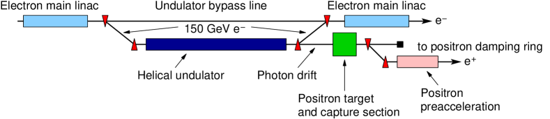
Figure 1: A concept for undulator-based production of polarized positrons at a linear collider.

In an alternative scheme the circularly polarized photons are produced by laser backscattering off an electron beam[10, 11], as has been proposed for the Japanese Linear Collider Project (JLC)[12, 13].

Experiment E166[14, 15] was performed to demonstrate that undulator-based production of polarized positrons can produce beams of sufficient quality for use in future linear colliders. Data were collected during two run periods in June and September 2005. A conceptual layout of the experiment is shown in Fig. 2 and details of the photon and positron diagnostics are given in Fig. 3.

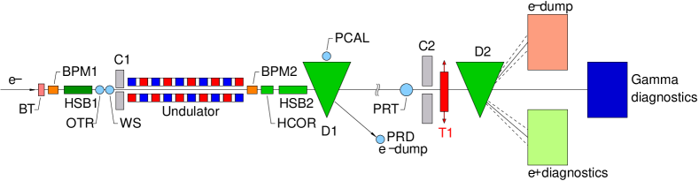
Figure 2: Conceptual layout (not to scale) of the experiment to demonstrate the production of polarized positrons in the SLAC FFTB. The electrons enter from the left and are dumped using magnet D1 after traversing the undulator. The positron-production target T1 and the positron and photon diagnostics are located 35 m downstream of the undulator. BPM = beam-position monitor; HSB = “hard” soft bend; OTR = optical-transition-radiation beam-profile monitor; BT = beam-current toroid; WS = wire scanner; C = aperture-limiting collimators; HCOR = horizontal-steering magnet; D1 = FFTB primary-beam-dump bend-magnet string; PCAL = positron calorimeter; PRD = dumpline beam-profile monitor; PRT = production-target beam-profile monitor; D2 = positron spectrometer.

The low-emittance, 46.6 GeV electron beam of the Final Focus Test Beam (FFTB)[16] at the Stanford Linear Accelerator Center (SLAC)[17] was passed through the undulator at 10 Hz to produce circularly polarized photons whose energy spectrum had its first-harmonic cutoff near 7.9 MeV. After the undulator, the beam electrons were deflected downwards to a dump by magnet D1. Positrons (and electrons) with energies in the range of a few MeV were produced by conversion of the undulator photons in a 0.8-mm-thick tungsten-alloy target T1.

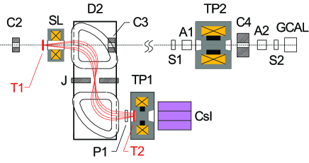
Figure 3: Schematic of the photon and positron diagnostics. A1, A2 = aerogel Cherenkov detectors, C2–C4 = collimators, D2 = dipole spectrometer magnet, CsI = $3\times 3$ array of CsI crystals, GCAL = Si-W calorimeter, J = movable W jaws, P1, S1, S2= Si-diode detectors, SL = solenoid lens, T1 = positron-production target, T2 = reconversion target, TP1 = positron-transmission-polarimeter solenoid, TP2 = photon-transmission-polarimeter solenoid. The detectors were encased in lead and tungsten shielding (not shown).

The helical undulator [18] was one meter long with a period of 2.54 mm and a strength parameter $K\approx 0.17$, as defined in Eq. (1). The helical coil was made by winding copper wires on a stainless-steel vacuum chamber with an aperture of 0.9 mm. The undulator was tested at currents up to 2300 A at 30 Hz repetition rate. During the data runs, it was operated at 10 Hz and 2300 A and delivered more than $4\cdot 10^{7}$ pulses without a single failure. The transformer oil in the undulator housing was replaced with a ferrofluid during part of the experiment, which yielded a 11% enhancement of the photon flux[19].

The undulator performance was characterized by measuring the total photon flux as a function of excitation current and the transmission of the photon beam through a 15-cm-long iron-core solenoid (transmission-polarimeter magnet TP2). A set of Si-W detectors S1–2 and GCAL and aerogel Cherenkov detectors A1-2 was used to measure the incident and transmitted photon flux and energy. The transmission asymmetry with respect to reversal of the polarity of magnet TP2 was affected by the spectral-transmission properties of magnetized iron and the polarization-dependent term of Compton scattering in the iron. These processes were modeled using a version of Geant3 that was modified to include the spin-dependent scattering effects. The measured fluxes and asymmetries agreed well with expectations based on MERMAID[20] calculations for the undulator strength and on the theoretical formulae for helical-undulator radiation.

The positrons created in target T1 were transported by a focusing solenoid SL to the entrance of a spectrometer D2 that separated the positrons from the incident photon beam and selected a narrow band of positron energies. The spectrometer, whose bend was in the horizontal plane, consisted of a pair of dipole magnets and adjustable tungsten-alloy jaws. The polarization of the positrons was measured by photon transmission polarimetry[21] after the positrons had produced photons in a thin tungsten “reconversion target” T2. These photons were passed through a 7.5-cm-long magnetized iron cylinder TP1. The photons leaving the analyzer magnet were much less collimated than in the case of the undulator photons. Therefore, a wider angular acceptance was obtained by use of a 3$\times$3 array of CsI crystals with a total cross section of about 180 mm$\times$180 mm. To simulate the positron polarimeter, Geant4[22, 23] was extended to include the relevant spin-dependent effects. These polarization extensions[24, 25] are part of Geant4 from v8.2 onwards.

Positron polarizations were measured at five energy settings of spectrometer D2. In addition, an electron-polarization measurement was made at a single energy setting by reversing the polarity of the spectrometer. Over the measured energy range of 4–8 MeV, the positron (and electron) polarization was about 80 % with a relative measurement error of about 10 % to 15 %, dominated by the systematic uncertainties[15]. The measured results agree well with expectations from detailed simulation of all aspects of the experiment.

The remainder of this paper describes in detail the experimental technique, data analysis and simulation, and the results of measurements of flux and transmission asymmetry of the undulator photons and of polarization of the positrons created from these photons.

2 Experimental Method

This section summarizes the principles of the methods used in this experiment for production of polarized photons and positrons, and for measurement of the longitudinal polarization of these particles.

2.1 Production of Polarized Photons in a Helical Undulator

Polarized positrons were produced in the present experiment by conversion in a thin target of circularly polarized photons with energy of a few MeV. The photons were produced by scattering of virtual photons of a helical undulator [8] with period $\lambda_{u}$ off an electron beam of energy $E_{e}=\gamma mc^{2}$, where $m$ is the mass of an electron, $c$ is the speed of light, and the electron beam is coaxial with the undulator. The highest energy photons take on the polarization of the undulator field, so that a helical undulator leads to circularly polarized photons.

The intensity of undulator photons depends on the intensity of the virtual photons of the undulator, and hence on the square of its magnetic field strength. It is conventional to measure the field strength of an undulator in terms of a dimensionless parameter $K$ defined as,

$$K=\frac{eB_{0}\lambda_{\rm u}}{2\pi\,mc^{2}}\cong 0.0934\,(B_{0}/1\,{\rm T})(\lambda_{u}/1\,{\rm mm}),$$ (1)

in which $e$ is the magnitude of the charge of an electron, and B₀ is the magnetic field on the axis of the undulator, which field is constant in magnitude while rotating through $360^{\circ}$ during each period $\lambda_{\rm u}$. The value of $K$ in the present experiment was small, about 0.17, because of practical limitations to the current in the (pulsed) undulator.

For small $K$-values, the number of photons $dN_{\gamma}/dL$ emitted per meter of an undulator and per beam electron is

$$\frac{{dN_{\gamma}}}{{dL}}\;\approx\;\frac{4}{3}\frac{{\pi\alpha}}{{\lambda_{u}}}K^{2}\;\cong\;\frac{{30.6}}{{\lambda_{u}/1\,{\rm mm}}}K^{2}\;\;{\rm photons/m/}e^{-},$$ (2)

where $\alpha$ is the fine-structure constant. The photon-number spectrum is relatively flat up to the maximum energy $E_{1}$ for scattering of a single virtual photon (dipole radiation of a beam electron),

$$E_{1} =\frac{2E_{e}^{2}\lambda_{\rm C}/\lambda_{\rm u}mc^{2}}{1+K^{2}+2\gamma\lambda_{\rm C}/\lambda_{\rm u}}\approx\frac{2E_{e}^{2}\lambda_{\rm C}/\lambda_{\rm u}mc^{2}}{1+K^{2}}$$

$$\cong 23.7\,\mbox{MeV}\frac{\left(E_{e}/50\,\mbox{GeV}\right)^{2}}{(\lambda_{\rm u}/1\,\mbox{mm})(1+K^{2})}\,,$$ (3)

where $\lambda_{\rm C}=h/mc=2.4\cdot 10^{-12}$ m is the Compton wavelength of the electron. The kinematic relation between energy and angle of emission of a real photon due to the scattering of $n$ virtual photons ($n^{th}$-order-multipole radiation) is, for small angles $\theta$ with respect to the electron beam,

$$E_{\gamma}(n,\theta)=\frac{nE_{1}}{1+(\gamma\theta)^{2}/(1+K^{2})}\;\;.$$ (4)

As seen from Eq. (4), the upper half of the energy spectrum at any order $n$ is emitted into a cone of angle $\theta=\sqrt{1+K^{2}}/\gamma$. The emission of photons due to higher-multipole radiation (with correspondingly higher energies) is suppressed for low values of $K$.

The photon-number spectrum $N_{\gamma}(E)$ is illustrated in Fig. 4(a)

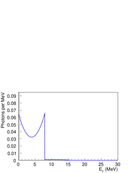
(a)

(b)

Figure 4: (a) The number spectrum $N_{\gamma}(E)$ of undulator radiation as a function of photon energy $E$, integrated over angle, for electron energy $E_{e}=46.6$ GeV, undulator period $\lambda_{\rm u}=2.54$ mm, and undulator-strength parameter $K=0.17$. The peak energy $E_{1}$ of the first-harmonic (dipole) radiation is 7.89 MeV. (b) The longitudinal polarization $P_{\gamma}(E)$ of the undulator radiation as a function of photon energy for an undulator with a right-handed helical winding.

for the experimental parameters: $E_{e}=46.6$ GeV, $\lambda_{\rm u}=2.54$ mm, $K=0.17$, and $E_{1}=7.89$ MeV. The number of photons generated is 0.35 per beam electron.

For the undulator photons produced at $\theta=0$ the longitudinal polarization is maximal, $P_{\gamma}=+1$ (for an undulator with a right-handed helical winding), but falls off for larger angles (which correspond to lower energies). This behavior is illustrated in Fig. 4(b) for the experimental parameters. The polarization of higher-harmonic radiation approaches unity at the corresponding higher cutoff energies, but the rates there are very low.

The average polarization of all undulator photons is nearly zero, but since higher-energy photons have higher polarization, the energy-weighted average polarization is 50 %.

Detailed descriptions of helical-undulator radiation can be found in[9, 26, 27, 28, 29].

2.2 Generation of Polarized Positrons

When a circularly polarized photon creates an electron-positron pair in a thin target, the polarization state of the photon is transferred to the outgoing leptons, as discussed by Olsen and Maximon in 1959[5]. Positrons with an energy close to the energy of the incoming photons are 100 % longitudinally polarized, while positrons with a lower energy have a lower longitudinal polarization (see Fig. 5).

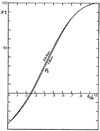
Figure 5: Longitudinal polarization of positrons (or electrons) produced by conversion of monochromatic circularly polarized photons in an infinitely thin target, as a function of the ratio $E_{e^{+}}/E_{\gamma}$ of positron to photon energies; from [5].

The sign of the positron polarization is opposite to that of the photon for positron energies less than 25 % of the photon energy.

The probability for the production of positrons is roughly independent of the fractional energy $E_{e^{+}}/E_{\gamma}$ in the pair-production process, so that positrons with all energies up to the photon energy are produced (with initial polarization as shown in Fig. 5). However, even in a thin target, low-energy positrons are stopped due to the ionization loss (which rises sharply for energies below 1 MeV), while high-energy positrons lose a fraction of their energy due to Bremsstrahlung. The energy loss by Bremsstrahlung is accompanied by a slight loss of polarization; however, the energy loss is more significant than the polarization loss. As a result, the low-energy portion of the positron spectrum is repopulated with positrons from the higher-energy portion, and the polarization of positrons of a given energy is higher in targets of up to $\approx 0.5$ radiation length than in an infinitely thin target[30], as shown in Fig. 6.

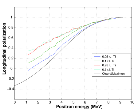
Figure 6: Longitudinal polarization of positrons produced by conversion of 10 MeV circularly polarized photons in targets of various thickness in radiation lengths, as a function of the positron energy.

For targets thicker than about 0.5 radiation length the polarization decreases again. Hence, positrons are nearly unpolarized in a conventional thick-target positron source even if the incoming photons are polarized.

The basic processes of polarization transfer in electromagnetic cascades (showers) are well known, but detailed understanding of the interplay of all processes in a shower is best obtained via numerical simulation with a Monte Carlo code. At the beginning of the experiment there was no code available that included all relevant processes. Therefore, a major effort was expended to implement polarization effects into the Geant4 code[24]. Details of the resulting simulations are reported in Sec. 4.

2.3 Photon Polarimetry

Measurements of the circular polarization of energetic photons are most commonly based on the spin dependence of their interaction with polarized atomic electrons[31, 32]. For photons of energy 1–10 MeV this interaction is dominantly Compton scattering. In this experiment, transmission polarimetry was used, i.e., measuring the transmission of unscattered photons through a thick, magnetized iron absorber[33, 21, 34], as sketched in Fig. 7.

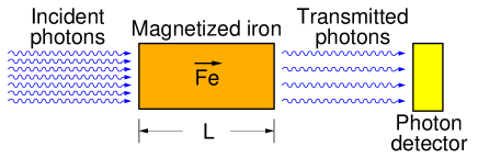
Figure 7: The concept of transmission polarimetry, in which the survival rate is measured for photons that pass through a magnetized iron absorber.

The Compton-scattering cross section for photons of energy $E$ in the MeV range off atomic electrons is taken to be that off free electrons,

$$\sigma(E)=\sigma_{0}(E)+P_{\gamma}(E)P_{e^{-}}^{\rm Fe}\sigma_{1}(E),$$ (5)

where $\sigma_{0}$ is the unpolarized (Klein-Nishina) cross section, $P_{\gamma}(E)$ is the net longitudinal polarization of the photons, $P_{e^{-}}^{\rm Fe}$ is the net longitudinal polarization of the atomic electrons, and $\sigma_{1}$ is the polarized cross section [33]. Figure 8 illustrates the energy dependence of the cross sections $\sigma_{0}$ and $\sigma_{1}$.

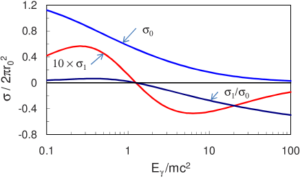
Figure 8: The total cross sections $\sigma_{0}$ and $\sigma_{1}$ of Eq. (5) for Compton scattering of longitudinally polarized photons of energy $E_{\gamma}$ off unpolarized and longitudinally polarized electrons, respectively; $r_{0}$ is the classical electron radius.

The average longitudinal polarization $P_{e^{-}}^{\rm Fe}$ of atomic electrons in an iron-core solenoid can be related to the average (longitudinal) magnetic field $\langle B-B_{0}\rangle$ of the iron, where $B_{0}$ is the part of the total magnetic field $B$ directly due to the current in the energizing coils, by

$$P_{e^{-}}^{\rm Fe}=\frac{\langle M_{s}\rangle}{n_{e}^{\rm Fe}\mu_{B}}=0.03727\langle B\,[{\rm T}]-B_{0}\,[{\rm T}]\rangle,$$ (6)

where $M_{s}=2(g^{\prime}-1)M/g^{\prime}=(0.958\pm 0.002)M$ [35] is the dominant spin part of the total magnetization $M=(B-B_{0})/\mu_{0}$, $g^{\prime}=1.919\pm 0.002$ is the magnetomechanical ratio as measured in Einstein-de-Haas-type experiments[36], and $\mu_{B}$ is the Bohr magneton. These expressions are also summarized in Table 1. Naively, $P_{e^{-}}^{\rm Fe}=\pm 2/26$ for saturated iron, but the number of aligned Bohr magnetons per atom is more accurately determined to be $2.218\pm 0.001$ for high-purity iron [37, 38] so that the maximum electron spin polarization in this material is $\pm 0.958\cdot 2.218/26=\pm 8.19$ %.

Table 1: Parameters and expressions relevant to electron polarization of magnetized iron.

Parameter	Expression
Electron polarization $P_{e^{-}}^{\rm Fe}$	$\langle M_{s}\rangle/(n_{e}^{\rm Fe}\,\mu_{B})$
	$=0.03727\langle B\,({\rm T})-B_{0}\,({\rm T})\rangle$
Magnetization $M$ (A/m)	$(B-B_{0})/\mu_{0}$
Spin fraction $M_{s}/M$	$2(g^{\prime}-1)/g^{\prime}=0.958\pm 0.002$
Magnetomechanical ratio $g^{\prime}$	$1.919\pm 0.002$
Electron number density $n_{e}^{\rm Fe}$	$N_{\rm A}\,\rho\,Z/A=2.206\cdot 10^{30}$ m-3
Bohr magneton $\mu_{B}$	$9.272\cdot 10^{-24}$ J/T
Vacuum permeability $\mu_{0}$	$4\pi\cdot 10^{-7}$ T-m/A

The transmission probability $T^{\pm}(E,L)$ for photons of energy $E$ and helicity $P_{\gamma}$ through a piece of magnetized iron whose length is $L$ can be written as

$$T^{\pm}(E,L)=e^{-n_{e^{-}}^{\rm Fe}L\sigma^{\pm}}=e^{-n_{e^{-}}^{\rm Fe}L(\sigma_{0}+\sigma_{\rm phot}+\sigma_{\rm pair})}e^{\pm n_{e^{-}}^{\rm Fe}LP_{e^{-}}^{\rm Fe}P_{\gamma}\sigma_{1}},$$ (7)

which takes also the cross sections for photoelectric effect, $\sigma_{\rm phot}$, and pair production, $\sigma_{\rm pair}$, into account. The $+(-)$ in $T^{\pm}$ applies if the electron spin in the iron is parallel (antiparallel) to the spin direction of the incident photons, and $n_{e^{-}}^{\rm Fe}$ denotes the number density of atoms in iron. The asymmetry

$$\delta(E,L)=\frac{T^{-}-T^{+}}{T^{-}+T^{+}}$$ (8)

in transmission of photons through the iron absorber when the sign of $P_{e^{-}}^{\rm Fe}$ is reversed, corresponding to a reversal of the magnetization of the iron, is

$$\delta(E,L)=\tanh\left(-n_{e^{-}}^{\rm Fe}L\,P_{e^{-}}^{\rm Fe}P_{\gamma}\,\sigma_{1}\right)\approx-n_{e^{-}}^{\rm Fe}L\sigma_{1}\,P_{e^{-}}^{\rm Fe}P_{\gamma}.$$ (9)

The sign convention in Eq. 8 results in a positive asymmetry $\delta$, given that the polarization-dependent Compton scattering cross section $\sigma_{1}$ is negative at the energies of this experiment. This asymmetry is shown in Fig. 9(a)

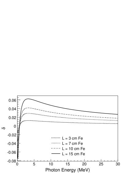
(a)

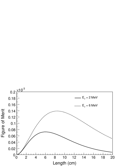
(b)

Figure 9: (a) The asymmetry $\delta(E,L)$ defined in Eq. (9) for transmission polarimetry of fully polarized photons on MeV energy $E$ in various lengths $L$ of saturated iron. (b) The figure of merit $\delta^{2}T$ for 2 MeV photons (solid) and for 6 MeV photons (dashed) as a function of the length of a transmission iron polarimeter.

for fully polarized photons incident on various lengths of saturated iron, using photon-iron cross sections from [39]. The peak asymmetry is in the range of 1–6 % for photon energies in the range of several MeV and for lengths of iron of 3–15 cm. For the photon polarimeter, where the rates were high, the length $L$ of magnet TP2 was chosen to be 15 cm to increase the size of the asymmetry.

An “analyzing power” $A_{\gamma}$ for transmission polarimetry can be defined as

$$A_{\gamma}(E,L)\equiv\frac{\delta(E,L)}{P_{e^{-}}^{\rm Fe}P_{\gamma}(E)},$$ (10)

where $A_{\gamma}\approx n_{e^{-}}^{\rm Fe}L\sigma_{1}$ for small asymmetries such that the final form of Eq. (9) holds. Then, a measurement of the asymmetry $\delta$, plus knowledge of the electron polarization $P_{e^{-}}^{\rm Fe}$ in the magnetized iron and of the analyzing power $A_{\gamma}$, would determine the photon polarization to be

$$P_{\gamma}=\frac{\delta}{P_{e^{-}}^{\rm Fe}A_{\gamma}}\,.$$ (11)

However, in the case of a broad distribution of photon energies, Eq. (10) becomes a convolution over energy-dependent detector efficiency, analyzing power, and photon polarization [40]. Correspondingly, the detectors in the photon line measure an effective polarization dominated by the high energy part of the undulator spectrum. To gauge the understanding of the polarization of the photon beam, the observed asymmetries, Eq. (8), will be compared with simulations.

2.4 Positron Polarimetry

The polarization of positrons could be determined in principle by observation of any polarization-dependent interaction of the positrons. For example, good precision can be obtained measuring Bhabha scattering in a thin, magnetized iron foil when the final-state electron and positron are detected in coincidence[41]. However, such a method is not applicable to the present experiment in which the positrons occur in pulses only a few-picosecond wide, such that coincidences are difficult to identify. Under these conditions, the simplest technique is the method of transmission polarimetry, in which the positrons are “reconverted” into photons which inherit the positron polarization (either by annihilation[42, 43] or by Bremsstrahlung[5, 44, 45]), and the photons subsequently pass through a thick iron absorber[46, 47, 48, 49, 50]. A measurement of the photon transmission asymmetry for magnetic fields (in the iron) parallel and antiparallel to the positron momentum vector then allows the polarization of the positrons to be inferred.

The transfer of polarization from positrons to photons (“reconversion”) in a thin foil is illustrated in Fig. 10.

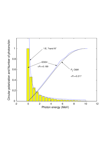
Figure 10: Solid curves: the polarization, as a function of energy, of photons generated by a 10 MeV positron incident on 0.5 mm of tungsten, according to an EGS4 simulation [51] and also to a calculation [5]. Histogram: the energy spectrum of the photons according to an EGS4 simulation. The photons are mainly due to Bremsstrahlung and their energies follow a $1/E$ “hand fit”; photons with energy above 10 MeV are due to annihilation.

The average polarization of the photons from a 10 MeV positron is only 21 % of that of the positron.

An asymmetry $\delta$ in the number of transmitted photons is measured by reversing the polarization $P_{e^{-}}^{\rm Fe}$ of the electrons in the iron absorber. The polarization $P_{e^{+}}$ of the parent positrons can then be inferred according to

$$P_{e^{+}}=\frac{\delta}{P_{e^{-}}^{\rm Fe}A_{e^{+}}}\,,$$ (12)

in terms of an analyzing power $A_{e^{+}}$ that can be calculated in a simulation which combines the processes of polarization transfer from positron to photon and transmission of the photons through the iron absorber. Because the reconverted photons have a nearly isotropic angular distribution (due to the large multiple scattering of the parent positrons in the reconversion target), the computation of the analyzing power $A_{e^{+}}$ is more complicated than for $A_{\gamma}$ in the case of transmission polarimetry of a collimated photon beam.

The relative error on the measurement (12) of the polarization varies inversely as the product of the asymmetry $\delta$ and the square root of the transmission factor $T=(T^{+}+T^{-})/2$. A figure of merit for transmission polarimetry can therefore be defined as $\delta^{2}T$, where larger values are better. This figure of merit is shown for 2 MeV photons in Fig. 9(b) as a function of length $L$ of the magnetized iron, which indicates that $L\approx 6$ cm maximizes the statistical significance of the asymmetry at this energy. The mean energy of the reconversion photons in the present experiment was 1–2 MeV, and the length of the positron polarimeter magnet TP1 was chosen to be 7.5 cm.

3 Experimental Setup

A schematic layout of the experiment is shown in Fig. 2. A 46.6 GeV electron beam generated polarized photons in the undulator. A set of bending magnets D1 deflected the high-energy electrons to a beam dump. The undulator photons were converted to electron-positron pairs in a thin target T1. Positrons and photons were analyzed in the apparatus sketched in Fig. 3 (and also in Fig. 11), while the low-energy electrons were dumped. Reversal of the spectrometer magnet D2 allowed for analysis of electron, while the positrons were in turn sent to the dump.

The remainder of this section presents details of the beamline, undulator, production target, photon and positron (or electron) diagnostics, data-acquisition system, runs types and data-file structure.

3.1 Beamline Layout and Alignment

The experiment required a high-energy, low-emittance electron beam to pass through a small-aperture, helical undulator to generate the polarized photon beam. Therefore, the experiment was performed in the Final Focus Test Beam (FFTB)[16] at SLAC [17], which could operate at energies up to 54 GeV and deliver an electron spot size of less than $50\times 50\ \mu$m² to an area appropriate for small experiments.

Figure 2 shows a schematic of the layout of the FFTB beamline elements specific to the experiment. Table 2

Table 2: Nominal and actual electron-beam parameters of the FFTB.

	$E_{e^{-}}$	$\gamma$	$f_{rep}$	$N_{e^{-}}$	$\gamma\epsilon_{x},\ \gamma\epsilon_{y}$	$\beta_{x}$, $\beta_{y}$	$\sigma_{x}$, $\sigma_{y}$	$\sigma_{x^{\prime}}$, $\sigma_{y^{\prime}}$	${\sigma_{E}}/{E}$
	(GeV)		(Hz)	($10^{9}$)	($10^{-5}$ rad)	(m)	($\mu$m)	($\mu$rad)	(%)
Nominal	50	$9.8\cdot 10^{4}$	30	20	3, 3	5.2, 5.2	40	13	0.3
Actual	46.6	$9.1\cdot 10^{4}$	10	1–4	2.2, 0.5	5.7, 19.8	35–40, 30–36	10, 1	$\sim$ 0.2

lists the nominal parameters of the FFTB beamline at the point where the undulator was installed, and the actual parameters achieved during running. The beam energy actually used, 46.6 GeV, was lower than nominal to insure more stable electron beam energy. The intensity was reduced to 1–$4\cdot 10^{9}\ e$/bunch to suppress the electron beam halo relative to the core beam, and thereby to decrease the relative size of backgrounds due to interaction of the tails of the beam with the 0.71-mm-diameter, 6.35-cm-long protection collimator C1. The reduced bunch intensity also permitted spot sizes slightly smaller than nominal.

Figure 11: Schematic of the experimental apparatus along the $\gamma$-line, including photon production in the undulator, conversion to $e^{\pm}$ in target T1, and subsequent diagnostics of photons and positrons. During the initial setup of the electron beam the bypass pipe was placed in the beamline rather than the undulator.

The undulator was preceded and followed by weak vertical-deflection magnets HSB1 and HSB2 that deflected the primary electron beam downward by $0.02^{\circ}$ each. This generated only a soft spectrum of synchrotron radiation along the undulator-photon line while decoupling this line from photons traveling with the primary electron beam upstream of the undulator. After HSB2, a string of seven permanent magnets D1 deflected the primary electron beam downwards by an additional $1^{\circ}$ and into the FFTB beam dump 45 m downstream of the undulator, as shown schematically in Fig. 2.

The electron-beam parameters were tuned using the beam-position monitors BPM1 and BPM2, the wire scanner WS and optical-transition-radiation monitor OTR to measure beam size, and toroid BT to measure the bunch charge.

The major challenge in operating the beam was to pass it through the extremely small aperture of collimator C1 (0.71 mm in diameter, 6.35 cm long), and then to maintain the beam tune so that the beam passed cleanly through the undulator during data-taking runs of 30–60 minutes each. The beam was initially set up using a 2.5-cm-diameter bypass beam pipe, shown in Fig. 11, instead of the undulator, and the beam orbit was recorded using the BPMs. Then the undulator was moved onto the beam orbit and aligned to a precision of a few $\mu$m using an array of five motion stages to minimize beam losses.

The undulator photons drifted in the $\gamma$-line, defined by the direction of the electron beam between magnets HSB1 and HSB2, for about 35 m to the diagnostic apparatus (Figs. 3 and 11), where they were either converted to electron-positron pairs in a thin target T1 (see Sec. 3.3) or analyzed (see Sec. 3.4). The undulator photons passed through tungsten collimator C2 (3 mm in aperture, 10.16 cm long) located 32.49 m downstream of the undulator center, which defined the transverse extent of the photon beam thereafter. The full width at half maximum of the undulator-photon beam was approximately 0.8 mm at collimator C2, based on Eq. (4) for the photon angular distribution and on the electron-beam parameters given in Table 2. Initial alignment of the electron beam (via horizontal- and vertical-correction magnets upstream), such that the $\gamma$-line passed through collimator C2 with maximal flux in detector S1, was accomplished using the bypass beam pipe and a beam of Bremsstrahlung photons generated by the 25-$\mu$m-thick (1-$\mu$m-thick in September 2005 run) Ti foil of the optical-transition-radiation monitor OTR.

Due to operational difficulties with the undulator motion stages, the electron beam was resteered slightly during much of the data collection to minimize backgrounds from collisions with collimator C1 and with the undulator itself. This steering resulted in partial loss of intensity in the $\gamma$-line due to reduced transmission through collimator C2.

3.2 Undulator

A single undulator, U1, was used throughout the experiment, although two complete undulator systems (Table 3) were fabricated and sent to SLAC.

Table 3: Parameters of the two fabricated undulator systems [18]. Only the system given in the first column (U1) was actually used in the experiment.

Parameter (Units)	U1	U2
Energy (GeV)	46.6	46.6
Length (mm)	1000	1000
Period (mm)	2.54	2.43
Number of periods	394	406
Aperture (mm)	0.87	1.07
Winding direction	left-handed	left-handed
Axial field (T)	$\sim 0.71$	$\sim 0.54$
$K$	$\sim 0.17$	$\sim 0.12$
$E_{1}$ (MeV)	$\sim 7.9$	$\sim 8.4$
Photons/$e^{-}$	0.35	0.18
$\Delta E/e^{-}$ (MeV)	1.65	0.88
Voltage (V)	$\sim 656$	$\sim 592$
Current (kA)	2.3	2.3
Pulse width ($\mu$s)	12	13
$\Delta T$/pulse (∘C)	$\sim 1.7$	$\sim 1.3$
Inductance ($\mu$H)	$\sim 1.4$	$\sim 1.5$
Resistance ($\Omega$)	$\sim 0.22$	$\sim 0.26$
Oil flow (l/min)	13.25	13.25
Press. drop (bar)	$\sim 0.76$	$\sim 0.76$

3.2.1 Undulator Fabrication

Six undulator coils were wound, three for each tube diameter, and each of these windings was tested at full current.

The undulator conductors were bifilar-helical windings with currents running in opposite directions (Fig. 12).

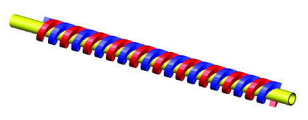
Figure 12: Sketch of the left-handed, bifilar windings of the undulator.

This method of helical-field generation, proposed in[8, 52], was used successfully some years ago[53] for an undulator with a period of 6 mm and $K\sim 0.35$.

The undulator conductor was oxygen-free CDA 10200 copper wire with square cross section $0.6\times 0.6$ mm² and corner radius $\leq 0.06$ mm. The wires were wound on hypodermic 304-L stainless-steel tubes with nominal OD’s of 1.07 mm (19-XTW) and 1.27 mm (18-XTW). All tubes had nominal wall thicknesses of 0.10 mm. Each tube was wrapped in Kapton insulation with a thickness of 12.7 $\mu$m. Four copper wires were wound onto a tube at a time: two of which were square cross section (bare) conductors, and the other two were of round cross section with 0.483 mm diameter and used as spacers. After completion of winding, the spacer wires were removed; it was found that the remaining conductors adhered to the tube without slippage. This procedure resulted in a period of 2.54 mm for the windings on 0.87-mm-diameter tubes, and 2.43 mm for those on 1.07-mm-diameter tubes.

All undulators were wound left-handed, i.e., counterclockwise as seen by a beam electron. This resulted in negative polarization $P_{\gamma}$ for the high-energy part of the undulator spectrum (see Sec. 2.1 and Fig. 4). Visual inspection of the undulators under a microscope allowed removal of tiny pieces of copper chips created in the winding process.

Even though the bending radius was of the order of the wire size, the keystone effect was not significant. A magnified view of windings is shown in Fig. 13.

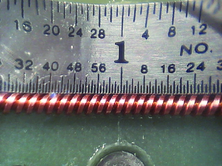
Figure 13: Photograph of the windings of undulator U1. The rectangular cross-section wire has dimensions of $0.6\times 0.6$ mm², and a period of 2.54 mm. The smallest scale division is 1/64 of an inch (0.397 mm).

Figure 14: Cross-section of an undulator system (dimensions in mm). Two G-10 rods (5) were placed in the corners of a long channel in an aluminum bar (3). A third rod (5) compressed the windings (2) to the other two rods via a spring-loaded bar (4). The Al undulator cover (1) was sealed with an indium gasket. The interior volume (6) was filled with oil or ferrofluid.

These windings were rather flexible and so were constrained by three cylindrical G-10 rods. Two of the rods sat in the lower corners of a U-shaped groove milled into an aluminum block and provided insulated support for the entire helix, as shown in Fig. 14. The third rod compressed the helical windings from above against the other two. The aluminum block had overall dimensions of $7.62\times 7.62\times 114.3$ cm³. The U-shaped groove was made to a tolerance of 12.7 $\mu$m throughout its length. This accuracy was achieved in a few milling steps after all flanges (with Al/stainless steel transitions) had been welded to the housing. The dimensions were checked commercially with a semi-automatic coordinate-measuring machine.

Two undulator bodies were milled simultaneously while attached to a baseplate by special holders which allowed expansion in the longitudinal direction. After fabrication, all Al parts were black anodized to minimize contact of the Al surface with oil. This procedure did not change the dimensions appreciably.

The routing of the leads to the helical winding, and of the “jumper” that closed the circuit at the end of the winding (Fig. 15), resulted in regions of net transverse magnetic field on the electron beam at the two ends of the undulator. In future fabrications, the extent of these regions should be minimized, and the directions of the transverse magnetic fields should be opposing.

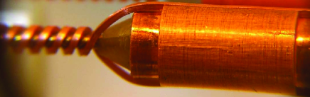
Figure 15: The downstream end of the undulator winding, showing the “jumper” that closed the circuit though a copper cylinder.

The aperture and straightness of the windings of undulators U1 and U2 was tested by stretching a 0.4-mm-diameter stainless-steel wire through the undulator and noting absence of electrical contact between wire and tube. For an electron-beam size of 40 $\mu$m, 0.4 mm is about $10\,\sigma$, sufficient for successful beam passage through the undulator. Further tests at SLAC measured the aperture of the undulator used in the experiment to be at least 0.71 mm.

3.2.2 Undulator Operation

Pure transformer oil was used as a coolant. The oil flowed in a circuit that included a stainless-steel oil pump, heat exchanger, reservoir, pressure gauges and valves. The oil flowed into the undulator case from the top center and exited at the lowest point in the groove below the G-10 rods (Fig. 14), also in the center. The oil pressure inside the case was about 2.4 bar, which expanded the chamber by a small amount.

The pumping/cooling system was constructed as a single mobile unit with oil pump, flow meters, heat exchanger, and 3-phase control electronics. This system could be operated locally or remotely and contained a set of thermal interlocks which ensured operational readiness of the system. A pressure transducer, PS 302-200GV, was attached to the line through a pressure snub, PS-4E, together with a DP25-SR strain gauge meter, also attached to the readiness interlock. The pressure transducer could be attached either to the outgoing or incoming line. The oil line was also equipped with dial-type pressure gauges installed near the undulator.

The undulator was connected to the cooling loop by oil-resistant, flexible tubes. The power supply was located in a rack together with the pulser in the FFTB tunnel.

The pulser is similar to the one used for the positron-production upgrade of CESR[54]. The undulator was tested at 2.3 kA and 30 Hz for one hour. This current represents the upper limit of the power supply (EMS800-2.5-5-D). Thus, in case of failure of all the electronics, the power supply would not deliver sufficient current to damage the undulator. The undulator was operated at 2.3 kA and 10 Hz with an average pulsed-current density of about 6.39 kA/mm², and a pulse duration of about 12 $\mu$s. The pulse waveform is shown in Fig. 16.

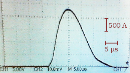
Figure 16: Current observed in the undulator shunt during a 2.3 kA pulse of $12\,\mu$s duration.

The current density in the undulator winding was calculated with the 3D code MERMAID [20]. This code calculated the current by solving for the electrostatic potential inside the conductor taking into account the actual geometry of the thick conductor. As the dimensions of the conductor were comparable to the bending radius, the current had a tendency to flow in layers closer to the center yielding a field enhancement on the axis. The current density varied by as much as a factor of four over the conductor cross-section. Wires with rectangular cross-section yielded a 15 % higher axial field compared to wires with circular cross-section.

The calculated field at the axis was $B_{\bot}\approx 0.71$ T at $I=2.3$ kA. As the measured period was $\lambda_{\rm u}\approx 2.54$ mm, the undulator factor $K$ defined in Eq. (1) was approximately 0.17. However, since the undulator pulse width was only about 12 $\mu$s at half height (Fig. 16), the skin depth was formally about 0.3 mm. Thus, the current had a tendency to be expelled from the interior of the conductor, which affected the magnetic field; but it is difficult to calculate the magnitude of this effect. An estimate of the undulator $K$ from direct measurements of the photon flux is presented in Sec. 6.1.

Towards the end of the data-taking run, the coolant oil was replaced with a ferrofluid (EMG 900) whose magnetic properties allowed it to serve as a return yoke for the magnetic field, thus increasing the effective undulator magnetic field. Calculations predicted a photon enhancement of about 20 %[19]. Data taken using the ferrofluid (Sec. 6.1.3) showed an enhancement of about one half this amount. The thermo-hydraulic properties of the ferrofluid are similar to those of oil, so no circulation or cooling problems were observed. The presence of the ferrofluid also increased the pulse rise time, which improved operation of the power-supply thyristors. At the end of the experiment the ferrofluid was found to be somewhat more radioactive than the normal oil.

The successful running of the present experiment verified the predicted undulator parameters and confirmed the engineering design principles.

3.2.3 Beam Deflection by the Undulator

A small deflection of the electron beam was observed when the undulator was energized in time with the beam. This had minimal impact on the present experiment, but such a deflection would be undesirable at a linear collider in which the electron beam passes through the undulator before colliding with the positron beam.

The deflection was first observed on an Al₂O₃(Cr) screen $\approx 42.9$ m downstream of the undulator, just upstream of the beam dump, where the beam spot was offset by $\approx 1$ mm for beam pulses in and out of time with the undulator. This angular deflection of about 25 $\mu$rad was corroborated by observation of small offsets of the electron beam in BPM2, just downstream of the undulator, that varied with the current in the undulator, as shown in Fig. 17.

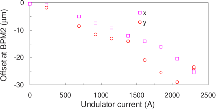
Figure 17: Offsets in $\mu$m of the electron beam at BPM2 as a function of undulator current.

The corresponding angular deflection at full current was about 25 $\mu$rad, assuming that the deflection occurred at the upstream end of the undulator, about 1.55 m from BPM2. Also, the PRT counters preceding collimator C2 showed a different displacement of background photons (from interactions of the electron beam with collimator C1 and/or the undulator) when the undulator was in and out of time with the electron beam.

It was concluded that the deflection was due to the routing of the leads at the upstream and downstream ends of the undulator, the latter of which is shown in Fig. 15, whose current may have introduced the $0.0039$ T$\cdot$m kick corresponding to the 25 $\mu$rad angular deflection. More careful design of the undulator leads should mitigate this issue. Imperfect alignment of the electron beam with respect to the undulator axis may also have contributed to the beam deflection.

3.3 Production Target T1

The left-handed undulator generated negative-helicity photons that passed through a tungsten collimator C2 with a 3-mm-diameter aperture before they struck the production target T1 where positrons were generated by pair production (see Figs. 3 and 11). The full width at half maximum of the photon beam was 0.9 mm at target T1. A five-position target holder provided for four targets, 0.2- and 0.5-radiation-length (r.l.) tungsten and titanium, and a no-target position. The tungsten was a sintered composite, W-4Ni-3Cu-3Fe, while the composition of the titanium alloy used was not specified (probably Ti-6Al-4V). Data were taken primarily with the 0.2 r.l. (0.81 mm) tungsten target, which provided both a good yield of positrons and good polarization transfer from the undulator photons, as shown in Fig. 6.

3.4 $\gamma$-Line

3.4.1 Overview

The $\gamma$-line and its associated photon diagnostics are shown in Figs. 3 and 11. Prior to impinging on the production target T1, undulator photons passed through a 3-mm-diameter, 10.16-cm-long, tungsten collimator C2, whose aperture defined the downstream $\gamma$-line. A set of four Si-W detectors (PRT) arrayed outside the aperture of collimator C2 was used to monitor the alignment of the $\gamma$-line. The photon flux from the undulator, after passing through collimator C2 and target T1, was measured independently by two counters, an aerogel Cherenkov counter A1 with an energy threshold of $\approx$ 4 MeV, and a Si-W counter S1 whose simulated response was utilized to provide normalization of the undulator-photon flux. A transmission polarimeter consisting of a 15-cm-long iron magnet TP2 (see Sec. 3.5.5), aerogel counters A2, and Si-W counter S2 detected effects of the polarization of the undulator photons. In addition, a Si-W calorimeter GCAL measured the total energy of the photon beam after the transmission polarimeter.

Photons from the undulator were measured by the Si-W detectors S1 and PRT whose absolute calibration was determined by Geant4 simulation as described in Section 3.4.2. The four PRT detectors were located immediately upstream of collimator C2 with edges tangent to the 3-mm-diameter collimator aperture, as shown in Fig. 18.

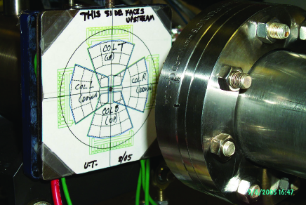
Figure 18: Placement of the quadrant detectors PRT1–4 upstream of collimator C2.

The shape and orientation of the individual detectors PRTtop, PRTright, PRTbottom, and PRTleft are shown in the photograph with the labels ColT, ColR, ColB, and ColL, respectively. The photon beam emerged from the $\gamma$-line vacuum window and entered the collimator from the right to the left. These detectors sampled that portion of the flux that does not enter the collimator aperture. They were installed between the June and September running periods to provide a measure of the centering of the undulator beam. The photons that exited collimator C2 struck the positron-production target T1 producing electron-positron pairs, and the unconverted photons were subsequently measured by detectors A1 and S1 prior to incidence on the polarimeter magnet TP2, after which the photon-transmission asymmetry was determined. With suitable correction, the sum of the fluxes through detectors A1 and S1 yielded the number of photons produced by the undulator per beam electron.

3.4.2 Particle Detectors

The particle detectors were required to deal with a rather wide range of energies and intensities. In the $\gamma$-line they measured undulator photons with intensities of 10⁷–10⁹ photons/pulse. In contrast, in the positron line typically a few thousand positrons per pulse were measured, leading to deposited energies of a few hundred MeV in the CsI calorimeter. Since asymmetry measurements of the form $A=(L-R)/(L+R)$ were utilized in the analysis of both photon and positron polarization, absolute calibration of detectors was not essential for the polarization analysis. However, to evaluate many quantities of interest, e.g., the number of undulator photons generated per beam electron, or to compare measured transmission with simulations, it was necessary to have a good understanding of the detector response functions.

Aerogel Counters:

The aerogel counters designated A1 and A2 in Figs. 3 and 11 were identical counters designed to detect undulator photons incident on, and transmitted through, 15 cm of magnetized iron (TP2). The sensitive elements were 2-cm-thick blocks of aerogel. The index of refraction of the aerogel was measured by interferometric techniques to be 1.0095 $\pm$ 0.0001, resulting in a Cherenkov threshold of 3.78 MeV. Cherenkov photons were reflected vertically by an aluminum mirror and passed through an air-filled light pipe to a photomultiplier tube. To prevent possible false asymmetries the photomultipliers were carefully shielded from background radiation and external magnetic fields.

Si-W Detectors:

The other detectors in the $\gamma$-line were based on silicon detector technology. The charge-sensitive elements were 300-$\mu$m-thick, reverse-biased, high-resistivity silicon layers (manufactured by Hamamatsu) mounted on 900-$\mu$m-thick G-10 supports. To enhance the sensitivity of these detectors to photons, each Si layer was preceded by a layer of tungsten (Densalloy SD170 [55].

It takes 3.66 eV for an electron or positron to create an electron-hole pair in silicon [56], and therefore 1 keV of energy deposited in a silicon detector liberated 4.38$\cdot$10^-5 pC of electrons. These electrons were collected in LeCroy 2249W ADCs after appropriate attenuation, required since the flux of $\approx 10^{9}$ photons per pulse in the $\gamma$-line led to large signals in the Si-W detectors.

The Silicon detectors in the $\gamma$-line were:

• S1, S2: These detectors were identical devices which counted incident and transmitted undulator photons (as did the Cherenkov counters A1 and A2). They consisted of a 555-$\mu$m-thick (0.13 r.l.) tungsten converter, and a single Si/G-10 detector. Under normal operating conditions the S1 signal was attenuated by 46–60 db and that of S2 by 20 db.

• GCAL: This device was a 9-element calorimeter, each element consisting of a 3.7-mm-thick ($\approx$ 0.9 r.l.) tungsten plate and a Si/G-10 detector, and provided a measure of the total energy of the transmitted photons. The GCAL signal was normally attenuated by 40 db.

• PRT: This was a set of four counters placed at the upstream edge of collimator C2, as shown in Figs. 2, 11 and 18. Each consisted of a 3.7-mm-thick tungsten converter and a Si/G-10 detector. Together they comprised a quadrant detector to aid in steering of the undulator-photon beam. They also provided an estimate of the fraction of undulator photons that did not enter the collimator aperture. The PRT signal was normally attenuated by 40 db.

Counter Comparisons:

The undulator flux that passed through collimator C2 was independently measured by counters A1 and S1 upstream of the iron-core solenoid TP2, and the transmitted flux was monitored by counters A2, S2 and calorimeter GCAL. While these detectors measure somewhat different features of the photon spectrum and had different sensitivities, good correlation was observed between signals in A1 and S1, as shown in Fig. 19 (a) for a sample of 290 runs during September 2005, and between A2, S2 and GCAL, as shown in Fig. 19 (b).

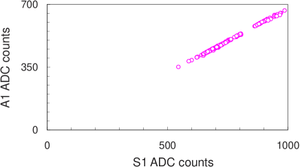
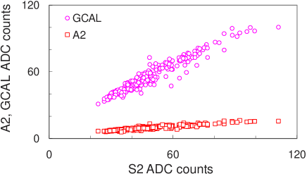
Figure 19: Comparison of signals in photon counters A1 and S1 (a), and in counters A2, S2 and GCAL (b).

3.4.3 PCAL Background Positron Monitors

A set of three 23-r.l.-long Si-W calorimeter units, PCALc, PCALd and PCALe, was placed above the dump magnet D1, about 10 m downstream of the undulator, as shown schematically in Fig. 2, to intercept energetic positrons from interactions of the tails of the primary electron beam with collimator C1 or with the undulator U1. The sensitivity of these calorimeter was a few hundred MeV per ADC count; thus, they were sensitive to interactions of individual beam particles. The PCALs were used to monitor the steering of the electron beam through the undulator aperture to minimize backgrounds in the downstream photon and positron detectors.

3.4.4 Other Background Detectors

Assorted other silicon detectors, CsI crystals and scintillator paddles were placed in the experimental area for background monitoring purposes; they were not essential to the operation of the experiment and they will not be discussed further.

3.5 Positron Transport and Diagnostics

Positrons were generated from undulator photons by pair production in a 0.81-mm-long tungsten production target (T1), and subsequently deflected with a double-dipole spectrometer (D2) into the positron analyzer, as shown in Figs. 3 and 11. A solenoid lens (SL) behind the production target increased the useful positron flux. A second tungsten target (T2) in front of the positron-polarimeter magnet (TP1) reconverted positrons to photons, so that the positron polarization could be inferred from that of the photons via transmission polarimetry. The transmitted, reconverted photons were detected in an array of CsI crystals.

Additional details of the positron transport are shown in Fig. 20.

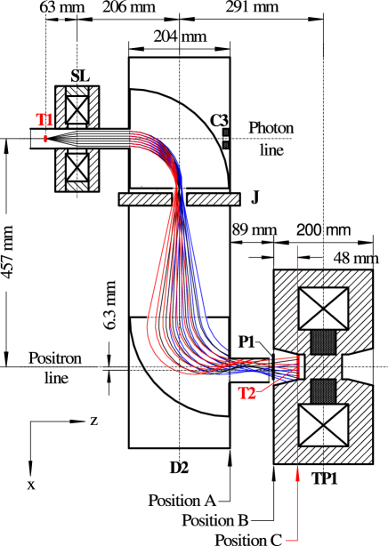
Figure 20: Top view of the positron/electron transport system showing the production target T1, the solenoid lens SL, the collimator C3 in the $\gamma$-line, the energy-selection jaws J and the vacuum chamber of spectrometer D2, the positron detector P1, and the positron reconversion target T2, together with nominal positron trajectories for the design energy selection of $\pm 5$ %.

During the experiment data were taken as a function of both the solenoid lens current $I_{\rm L}$ and the dipole spectrometer current $I_{\rm S}$. The five sets of currents used for the positron analysis are summarized in Table 4. The lens currents $I_{\rm L}$ were chosen to obtain maximal positron yield in detector P1 for each spectrometer current $I_{\rm S}$. Electron analysis was performed only for $I_{\rm S}=160$ A by reversing the spectrometer current (but not reversing the corresponding solenoid current). Data were collected with ferrofluid in the undulator only for positrons with $I_{\rm S}=180$ A.

Table 4: The currents $I_{\rm S}$ in the dipole spectrometer and $I_{\rm L}$ in the solenoid lens used for positron analysis in the experiment and in the Geant4 simulations (Sec. 4). The lens currents $I_{\rm L}$ were chosen to obtain maximal positron yield for each spectrometer current $I_{\rm S}$. Electron analysis was performed only for $I_{\rm S}=160$ A by reversing this current. The central positron energy $E_{e^{+}}$ selected by the spectrometer as simulated with Geant4 is compared with the values calculated from a calibration with a ⁹⁰Sr $\beta$-source. The range of energies in column five reflects the uncertainty in the determination of the endpoint of the $\beta$ spectrum.

$I_{\rm S}$ (A)	$I_{\rm L}$ (A)	$I_{\rm L}$ (A)	$E_{e^{+}}$ (MeV)	$E_{e^{+}}$ (MeV)
expt.	expt.	Geant4	Geant4	90Sr $\beta$
100	220	225	4.59	4.42 - 4.84
120	260	250	5.36	5.14 - 5.62
140	340	300	6.07	5.81 - 6.36
160	360	325	6.72	6.45 - 7.06
180	374	350	7.35	7.05 - 7.72

The central positron energies corresponding to the spectrometer currents $I_{\rm S}$ were confirmed by placing a ⁹⁰Sr source at the position of the production target T1, which showed that the highest current for which a signal was detected at counter P1 (see Figs. 3 and 11) was 52 A. The nominal endpoint of the $\beta$ spectrum was 2.752 MeV, but after correcting for energy loss in source windows and spectrometer air it was determined that $E_{e^{-}}=2.515\,$MeV ($p_{e^{-}}=2.462$ MeV/$c$) corresponded to a spectrometer current of $I_{\rm S}=50.5\pm 1.5\,$A. The range of energies reported in column 5 of Table 4 were scaled from this result using Eq. (17) to characterize the slightly nonlinear dependence of the spectrometer magnetic field on current.

3.5.1 Solenoid Lens SL

The solenoid lens SL provided a point-to-parallel transport of positrons from the production target T1 to the entrance of the dipole spectrometer D2. The solenoid coils were four double pancakes with 14 radial turns each, wound using a square copper conductor with a cross section of $4.76\times 4.76\,{\rm mm}^{2}$, an inner, circular water channel of 3.175 mm diameter, and a conductor area of 13.9 mm². The coil thickness, including insulation, was 44.6 mm. The coils were housed in a 1010-iron flux return, about 20 mm thick, with overall length of 88.6 mm and outer radius of 106.5 mm. The lens carried current $I_{\rm L}$ up to 374 A, corresponding to a maximum current density of 27 A/mm². Cooling water was circulated through the coils with a pressure differential of 5 bar, such that the operating temperature of the solenoid was only slightly above ambient.

Magnetic Field:

The magnetic field of the solenoid lens (and of the spectrometer dipoles) was initially modeled with the 3D-code MERMAID[20], which is based on a finite-element algorithm that takes into account the geometry and the magnetic properties of different components of a given setup. At the conclusion of the experiment the field of the lens was mapped by the SLAC Magnetic Measurements group, who measured along the $z$-axis for different $x$-positions (using a one-dimensional Hall probe, providing only the component $B_{0}(z)=B_{z}(r=0,z)$. The $(x,y,z)$ coordinate systems used here have the $z$-axis parallel to the $\gamma$-line (which tilted downwards at an angle of about $0.3^{\circ}$), the $x$-axis horizontal, and the $y$-axis (nearly) vertical. A complete field map of the components $B_{r}(r,z)$, and $B_{z}(r,z)$ in the current-free space inside the solenoid was extrapolated to second order (assuming azimuthal symmetry) via Maxwell’s equations from the field measured on-axis:

$$B_{r}(r,z) =-\frac{r}{2}\left(\frac{dB_{0}(z)}{dz}-\frac{r^{2}}{8}\frac{d^{3}B_{0}(z)}{dz^{3}}\right),$$ (13)

$$B_{\phi} =0,$$ (14)

$$B_{z}(r,z) =B_{0}(z)-\frac{r^{2}}{4}\frac{d^{2}B_{0}(z)}{dz^{2}}.$$ (15)

The measured and extrapolated field maps agree well with a computation using MERMAID. The parametrization of Eqs. (13)–(15) was used in the simulations described in Sec. 4.

3.5.2 Dipole Spectrometer D2

The dipole spectrometer D2 was designed to select and transport a 5 % energy bite of positrons (or electrons) to a second beamline offset by 46 cm from the $\gamma$-line, such that positron polarimetry could be carried out in a low-background environment.

The spectrometer was a system of two opposite-polarity dipole magnets separated by a 25.4 cm drift space (see also Fig. 20) such that the total angular deflection was approximately zero while the transverse displacement was 46.4 cm. The resulting “dog leg” beam transport included an intermediate focus close to the exit of the first dipole, at which point 25.4-mm-thick tungsten jaws were placed to select the energy of the positrons via remote control of the separation (normally 30 mm) of the jaws.

The spectrometer contained a vacuum chamber that included the production target T1, a cylindrical entrance pipe of 36 mm inner diameter that passed through the solenoid lens, and a cylindrical pipe of 48 mm inner diameter at the exit of the spectrometer. The entrance window, upstream of target T1, was 25 mm in diameter, and the exit window was 50 mm in diameter; both windows were 25-$\mu$m-thick stainless-steel foils. The vacuum chamber was fabricated such that the offset between the entrance and exit pipes was 464 mm, rather than 457 mm as designed, which resulted in some occulting of the positron beam by the exit pipe, as discussed further in Sec. 4.3.

The magnet poles were machined as quadrants of a cone of radius 20 cm and height 3.8 cm to provide vertical focusing in the entrance and exit fringe fields. The smallest gap between the poles was 5.33 cm, into which gap a vacuum chamber was inserted. Within each dipole the central orbit was a circle of radius $R_{0}\approx 13.1\,{\rm cm}$. The tapered magnet gaps resulted in a field gradient with a slope factor near the central orbit

$$n=-\frac{R_{0}}{B_{0}}\frac{\partial B}{\partial r}\approx 0.5.$$ (16)

The coil of each magnet pole was wound with $6\times 6$ turns of the same square copper conductor used in the solenoid lens. The two dipoles were energized in series, and the flux of each magnet passed through the other via iron return-yoke plates above and below the magnet poles.

The magnet poles were faced with DEN23 tungsten (Tungsten Products, Madison, AL, USA) machined to the inverse of the shape of the poles. The nominal magnetic permeability of the tungsten was less than 1.05, but consistency between measurements and calculations of the magnetic field in the spectrometer (see below) indicated that the permeability was close to 4. This deviation from its design value led to modifications of the beam trajectories in the spectrometer, as discussed further in Secs. 3.5.3 and 4.3.4.

Magnetic field:

The spectrometer magnetic field was calculated using the MERMAID program[20], and was also mapped by the SLAC Magnetic Measurement group at the conclusion of the experiment. The measured field map consisted of ten parallel $(x,y)$ planes that were grouped into a 3D lattice covering the region from the production target through the spectrometer to the polarimeter section. The calculated magnetic field is in good agreement with the results of field measurements. Figure 21

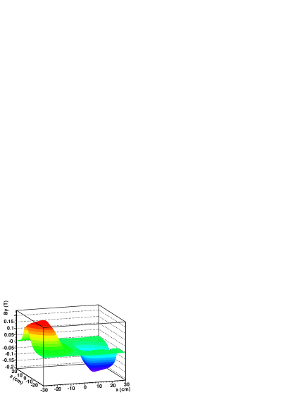
Figure 21: Profile of the vertical magnetic-field component $B_{y}$ of the dipole spectrometer vs. $x$ and $z$ in horizontal midplane $y=0$.

shows the profile of $B_{y}$ in the $(x,z)$ plane at $y=0$.

A field map was calculated using MERMAID for a spectrometer current of $I_{\rm S}=150\,$A. In the absence of saturation effects the magnetic field $B_{y}$ would change linearly with the current. Hall-probe measurements of field vs. current at several locations revealed a nonlinear dependence of the form

$$B_{y}(I_{\rm S})=a\cdot I^{2}_{S}+b\cdot I_{\rm S}+c,$$ (17)

with $a=-1.684\cdot 10^{-6}$ T/A², $b=1.536\cdot 10^{-3}$ T/A and $c=1.841\cdot 10^{-3}$ T. At the highest current, 180 A, the field was about 20 % less than that expected for linear behavior. The field maps used for current $I_{\rm S}$ in the simulations (Sec. 4) were obtained by scaling the MERMAID map at 150 A by the factor $B_{y}(I_{\rm S})/B_{y}(150\,{\rm A})$ according to Eq. (17).

3.5.3 Positron Monitor P1

Silicon detector P1 was placed between the exit window of the spectrometer and the positron reconversion target T2 (see Fig. 20) to measure the positron flux and spatial distribution. It consisted of a single 300-$\mu$m-thick layer of silicon that was read out in four quadrants. The counter’s sensitivity was about 49 positrons per ADC count, and typical signals were a few hundred counts/pulse.

Experimental data from the Si-W detector P1, which was read out in quadrants, showed that 90–95 % of the positrons passed through its left half, as summarized in Table 5 and illustrated graphically in Fig. 22.

Table 5: Fraction in percent of particles observed in the quadrants of detector P1 for the various spectrometer currents. ff = ferrofluid.

$I_{\rm S}$ (A)	top/left	top/right	bottom/left	bottom/right
100	46.8	3.0	46.8	3.3
120	45.8	2.6	48.9	2.6
140(1)	41.9	3.1	48.2	6.8
140(2)	42.3	2.7	52.2	2.9
160(e+)	38.2	2.4	56.5	2.9
160(e-)	69.7	3.9	23.2	3.2
180	34.9	2.8	58.8	3.5
180(ff)	38.0	2.8	55.8	3.5

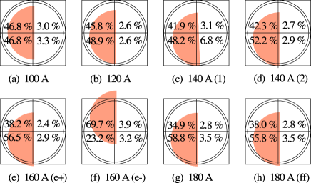
Figure 22: Representation of the distributions of positrons at the P1 quadrant detector listed in Table 5, assuming that the positrons uniformly populated a half-circular region.

This was caused by deviations of the spectrometer properties from their design specifications, as described above and discussed further in Sec. 4.3.4. The distribution of electrons was shifted upwards with respect to that of positrons.

3.5.4 Positron Reconversion Target T2

To determine the polarization of the positrons, they were converted back into photons and the polarization of the latter was measured in a transmission polarimeter based on the iron-core magnet TP1. A 2-mm-thick tungsten composite (Densimet D17k, with a nominal composition of 90.5 % W, 7 % Ni, 2.5 % Cu) target, T2, was placed 12.5 mm upstream of the magnet to convert most of the positrons into photons, although some positrons were only converted after they entered the iron magnet.

3.5.5 Polarimeter Magnets

Iron-core solenoid magnets were employed for the measurement of the photon and (reconverted) positron beam polarizations according to Eqs. (11) and (12), where the average longitudinal polarization $P_{e^{-}}^{\rm Fe}$ of atomic electrons in the iron is related to longitudinal magnetic field $B$ according to Eq. (6).

The iron core of the positron analyzer TP1 was 50 mm in diameter and 75 mm in length, as shown in Fig. 23, while that of the photon analyzer TP2 was 50 mm in diameter and 150 mm in length.

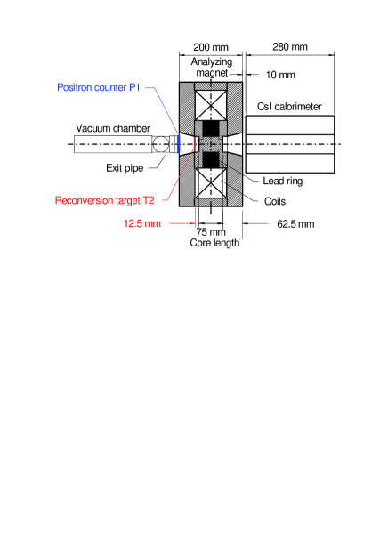
Figure 23: Sketch of the positron polarimeter. Positrons entered from the left, passing in succession through the exit window of the spectrometer, the Si-W counter P1, the reconversion target T2, after which the reconverted photons passed through the iron-core magnet TP1 and were absorbed in the CsI calorimeter on the right.

These magnets were fabricated at the Efremov Institute [57] based on modeling which showed that the iron would be saturated over most of the cylindrical core, as shown in upper part of Fig. 24.

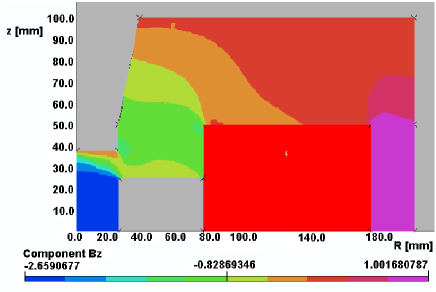
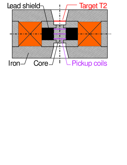
Figure 24: Top: 2d-field model in the $r$-$z$ plane of magnet TP1. Bottom: Horizontal section of magnet TP1 showing the location of the pickup coils. The top figure corresponds to the first quadrant of the bottom figure.

Photons traversing the structure outside the core region were strongly suppressed, as they encountered more iron and an additional lead shield (see Figs. 23 and 24).

The main parameters of the polarimeter magnets TP1 and TP2 are listed in Table 6.

Table 6: Parameters of the polarization analysis magnets TP1 and TP2.

Parameter (Unit)	TP1	TP2
Overall length (mm)	200	275
Overall diameter (mm)	392	320
Iron-core length (mm)	75	150
Iron-core diameter (mm)	50	50
Length of internal Pb absorber	50	125
Overall mass (kg)	175	195
Number of coils	2	2
Coil length (mm)	49	86
Coil inner diameter (mm)	152	152
Coil outer diameter (mm)	322	248
Number of turns per coil	160	175
Conductor dimensions (mm)	$4\times 4$	$4\times 4$
Coolant bore diameter (mm)	2.5	2.5
Water cooling circuits	4	4
Water flow rate (l/min)	$\sim 2$	$\sim 2$
Operating current (A)	$\pm 60$	$\pm 60$
Power (kW)	1.62	1.37
Current reversal time (s)	1.0	1.0
Time between reversals (min)	5	5
Field $B_{z}^{\rm max}$ at center (T)	2.324	2.165
On-axis mean field $\left\langle B_{z}\right\rangle$ (T)	2.071	2.040
Air field $B_{0}$ at center (T)	0.097	0.100
Number of pickup coils	3	3
Pickup-coil diameter (mm)	48.5	48.5
Number of turns per pickup coil	160	160
$z$-Position of pickup coils (mm)	0, $\pm 20$	0, $\pm 57.5$
$\left\langle P_{e^{-}}^{\rm Fe}\right\rangle$ (on axis)	0.0736	0.0723
	$\pm 0.0015$	$\pm 0.0015$

Both magnets were energized through fast linear amplifiers[58] which permitted rapid polarity reversal. For transmission polarimetry, the field direction was automatically reversed every 5 minutes with a linear current ramp over 1 second, as shown in Fig. 25.

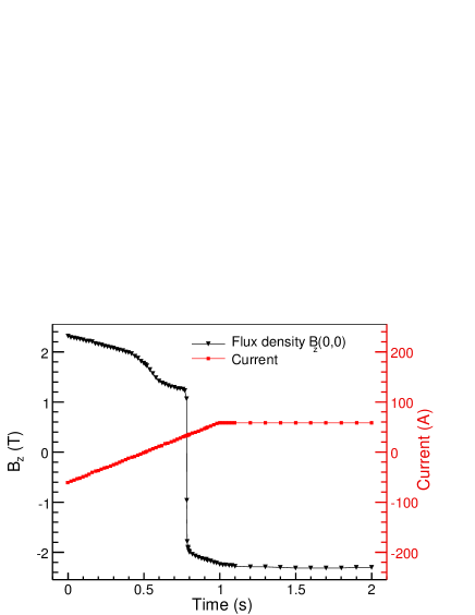
Figure 25: OPERA-2d [59] calculation of the field in magnet TP1 for a linear current ramp from $-60$ A to $+60$ A over 1 s.

The nonlinear response was due to eddy effects.

Magnetic Field:

The magnetic field of the iron was measured and monitored with several pickup coils surrounding the core of each magnet, shown for magnet TP1 in the bottom part of Fig. 24. The induced-voltage signal $V(t)=d\Phi/dt$, where $\Phi$ is the magnetic flux through the pickup coil, upon field reversal was digitized at a readout frequency of 50 Hz[60]. An additional pulse with triangular shape from a waveform generator with known repetition frequency was used to calibrate the time scale of these measurements. An example of these magnetic flux measurements is shown in Fig. 26.

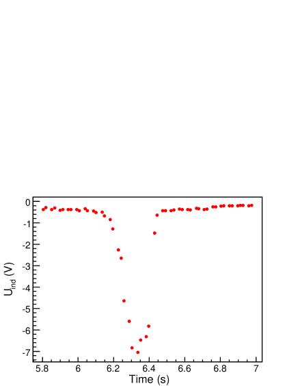
(a)

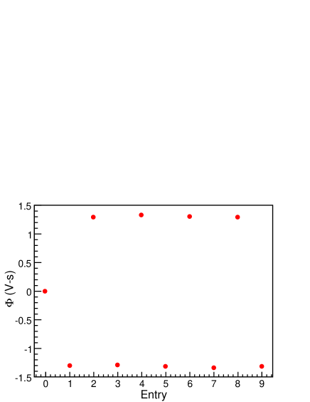
(b)

Figure 26: Induced-voltage signal upon field reversal in one of several pickup coils surrounding the iron core of magnet TP1: (a) voltage vs. time (left); (b) Magnetic flux $\Phi=\int Vdt=BA$ for several polarity flips (right).

An excitation curve of flux vs. current is shown in Fig. 27

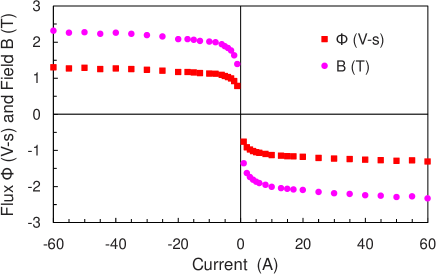
Figure 27: Flux measurements and derived field values at the center of magnet TP1 as a function of magnet current.

for the central core region of the positron analyzer. The magnetic field $B$ was obtained from the time integral of the induced voltage, $\int Vdt=\Phi=BA$, and the known cross section area $A$ of the pickup coil. The central magnetic field at the operating current of $\pm 60$ A was determined in this way to be 2.324 T for the positron analyzer, and 2.165 T for the photon analyzer, with a typical relative measurement error of 1 %.

To obtain $\langle B_{z}\rangle$ averaged over the entire cylindrical core volume, detailed field modeling was performed with the OPERA-2d code[59]. The nominal $B$-$H$ curve for the soft magnet iron (1010 steel) was adjusted until satisfactory agreement with the measured fields in the pickup coils was obtained. Results of the field modeling of the positron analyzer are shown in Fig. 28,

Figure 28: Longitudinal field component $B_{z}$ in the positron analyzer (modeled with OPERA-2d [59]) as a function of $z$ for different radial distances from 0 to 22.5 mm.

which plots the longitudinal field component $B_{z}$ as a function of $z$ for different radii. The center of the core is at $z=0$, and the end faces are located at $\pm 37.5$ mm. At the operating current of 60 A, the core remained near its central saturation value $B_{z}(0,0)=B_{z}^{\rm max}=2.324$ T for much of its length. Near the exit face at $z=\pm 37.5$ mm, however, the longitudinal field component diminished more or less rapidly, depending on the radial distance. This general behavior is also apparent in the 2d-field distribution shown in Fig. 24. For photons propagating on axis or with a constant radial offset, the average $\left\langle B_{z}\right\rangle$ is listed in Table 7.

Table 7: Field integrals and average electron polarization of the magnetized iron core. For the positron analyzer the integration covered a cylindrical volume of radius $r$ and the full core length of 75 mm along $z$. For the photon analyzer only the axial case was evaluated for the full core length of 150 mm.

Radius	$\langle B_{z}\rangle$	$\langle B_{z}-B_{0}\rangle$	$\langle P_{e^{-}}^{\rm Fe}\rangle$
(mm)	(T)	(T)
Positron Analyzer TP1
$r=0$	2.071	1.974	0.0736 $\pm$ 0.0015
$0<r\leq 5$	2.046	1.949	0.0726 $\pm$ 0.0015
$0<r\leq 10$	2.025	1.928	0.0719 $\pm$ 0.0015
$0<r\leq 15$	2.001	1.904	0.0710 $\pm$ 0.0015
$0<r\leq 20$	1.977	1.880	0.0701 $\pm$ 0.0015
$0<r\leq 22.5$	1.963	1.866	0.0695 $\pm$ 0.0015
Photon Analyzer TP2
$r=0$	2.040	1.940	0.0723 $\pm$ 0.0015

To account for possible systematic effects from fringe fields on positron or electron trajectories, a detailed field map was also generated for the exterior air space surrounding the positron analyzer, which served as input to simulation studies. Figure 29

Figure 29: The magnitude $|B|$ of the fringe-field distribution in the first quadrant of the $r$-$z$ plane of the positron analyzer TP1 (bottom part of Fig. 24), as modeled with OPERA-2d [59].

shows the magnitude $|B|$ of the fringe field in the $r$-$z$ plane, based on a computation of the axial and radial field components. At the reconversion target ($z=52$ mm), a fringe field of 44 mT was determined from the model. Further out, it dropped to 1 mT at the start of the trombone-shaped entry throat ($z=100$ mm), which was the location of the positron counter P1 (Fig. 23). These field values have been confirmed with Hall-probe measurements.

The electron spin polarization $P_{e^{-}}^{\rm Fe}$ of the iron is proportional to $\langle B-B_{0}\rangle$ according to Eq. (6), where $B_{0}$ is the “air field”, due to the current in the magnet coils, that would exist in the absence of the iron. The air field $B_{0}$ was calculated from the known solenoid parameters shown in Table 6, and was about 5 % of B. As the air field varied in the core region by less than 11 % from its central value, it was sufficient to use a constant air-field correction with a systematic error of less than 0.5 % in $P_{e^{-}}^{\rm Fe}$.

The polarization of atomic electrons in iron was calculated from the measured magnetic fields according to Eq. (6) as $P_{e^{-}}^{\rm Fe}=0.03727\langle B\,[{\rm T}]-B_{0}\,[{\rm T}]\rangle$, with results summarized in Table 7. On axis, the average electron polarization was $0.0736\pm 0.0015$ for the positron analyzer TP1, and $0.0723\pm 0.0015$ for the photon analyzer TP2. The errors reflect uncertainties in the field measurements and field modeling. Away from the axis there was a slight drop in the average polarization, as detailed in Table 7 for the positron analyzer. For the photon analyzer only the on-axis field was relevant, since the beam was narrowly collimated in that case.

Although the average $P_{e^{-}}^{\rm Fe}$ over the iron core of magnet TP1 was known to $\pm\,0.0015$ (Table 7), the systematic uncertainty was taken to be $\Delta P_{e^{-}}^{\rm Fe}=0.0021$ (i.e., 3 %) to account for uncertainties in the knowledge of the spatial distribution of the photons within the cylindrical core.

3.5.6 The CsI(Tl) Calorimeter

The total energy of each pulse of photons that emerged from the analyzer magnet TP1 after the positron reconversion target T2 was measured by a CsI(Tl) calorimeter (shown in Figs. 3, 11, and 23) made of nine crystals arranged in a 3$\times$3 array.

Crystals:

The most important properties of the crystals (supplier: Monokristal Institute, Kharkov, Ukraine) are summarized in Table 8.

Table 8: Parameters of the CsI(Tl) crystals.

Thallium (dopant)	0.08 mol %
Light yield	4000–5500 photons/MeV
Peak emission wavelength	550 nm
Length	280 mm (15.11 r.l.)
Height	60 mm
Width	60 mm

The homogeneity of the light yield was tested[61] by moving a ⁶⁰Co source along the sides of the crystals and analyzing its spectrum. From 14 measured points per crystal the homogeneity of each crystal was found to be within 10 % of the average in most cases, with some exceptions (Fig. 30).

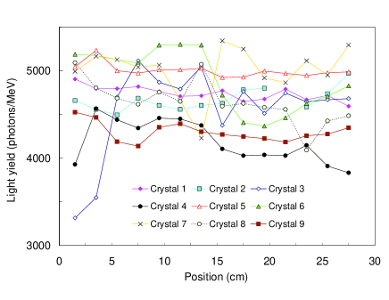
Figure 30: The photoelectron yield per MeV vs. longitudinal position for the nine CsI(Tl) crystals.

The average light yield of the nine crystals was found to vary between 4000 and 5500 photons per MeV of deposited energy. This variation was accounted for in the calibrations of the individual crystals.

Mechanical Assembly:

Each crystal was wrapped with two layers of white Tyvek paper, which provided diffuse reflections at the crystal walls and increased the scintillation light collection. To avoid cross-talk between the crystals, each one was additionally wrapped with a thin copper foil (30 $\mu$m) which also acted as an electromagnetic shield. The wrapping caused about 1.2 mm of dead space between the crystals. The crystals were stacked with the use of plastic spacers inside a brass chamber with 6 mm wall thickness. The front wall, facing the analyzer magnet, was thinned down to 2 mm in the sensitive area. The box was light-tight but not air-tight (a hygroscopic material inside the box kept the humidity low).

Ninety percent of the energy of the reconverted photons was deposited in the central CsI crystal, so the crystal with the highest light yield was placed in the center of the array. The next-best-quality crystals were used as the four neighbors of the central crystal, and the four corner crystals had the lowest quality.

Electronic Readout:

The front end of the electronic readout of the scintillation light (Fig. 31)

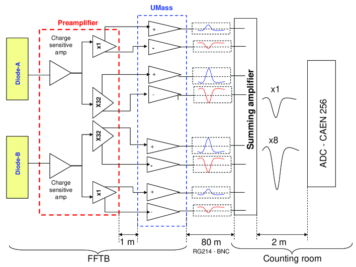
Figure 31: Scheme of the readout electronic chain: photodiode, preamplifier, UMass board, summing amplifier and ADC.

was adapted from the BaBar experiment[62]. A module of two photodiodes (called A and B in Fig. 31) with a total active area of 20$\times$20 mm² was coupled to the crystal via a thin polystyrene plate using an optical grease. The PIN diodes (Hamamatsu model S2744-08) were operated with a reverse bias voltage of $-50$ V with the cathode grounded. Typical values for the dark current of 3 nA and a capacitance of 85 pF for the doublet were reported by the manufacturer. The signals from each diode were fed into charge-sensitive preamplifiers, each with two bipolar outputs, one with low gain (LG, gain 1) and the other with high gain (HG, gain 8).

These bipolar signals were fed via flat cables (about 1 m long) onto the so-called UMass board (adapted from a BaBar crystal test setup) which drove a total of 72 coaxial cables (one for each polarity of the bipolar signals) over a length of 80 m from the FFTB tunnel to the counting room. There, a summing amplifier (custom made for this experiment) combined the two polarities of each signal by adding the inverse of the positive signals to the negative ones, and by adding the signals with the same gains from diodes A and B of a crystal. The resulting 18 pulses were attenuated by 40 dB and then digitized by three, 8-channel, charge-integrating ADCs (CAEN model V265). The digital output of each ADC channel was two 12-bit words, where the second word was obtained from digitization of the input signal with 8 times higher gain, corresponding to 15-bit resolution over the range of the 12-bit word. Thus, digitized signals from each CsI crystal were recorded for four resolutions, designated as LG-LS (Low Gain - 12 bits), LG-HS (Low Gain - 15 bits), HG-LS (High Gain - 12 bits), and HG-HS(High Gain - 15 bits). However, in the final analysis only the 12-bit-resolution data taken with low gain (i.e., LG-LS) were used.

Energy Calibration:

The typical energy deposition in a CsI crystal by photons from reconverted positrons was a few hundred MeV per electron-beam pulse.

Prior to data taking with beam, calibration constants for the calorimeter were obtained from high-statistics spectra of cosmic-ray muons using HG-HS resolution, as illustrated in Fig. 32(a). They were confirmed for the outer eight crystals via ²²⁸Th decays (2.861 MeV photo peak) at the same resolution but with only 20 dB attenuation of the signals (Fig. 32(b)).

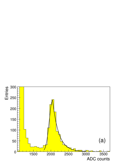
(a)

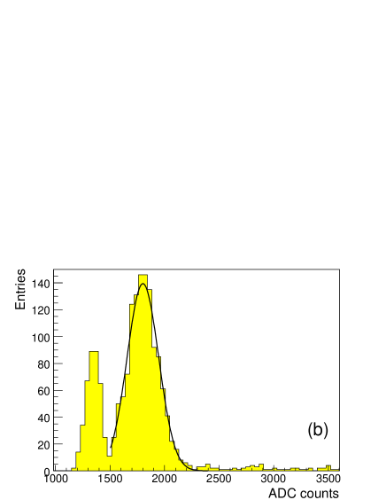
(b)

Figure 32: Examples of calibration spectra from CsI crystal 8. (a): Cosmic-muon spectrum (40 dB attenuation); (b): ²²⁸Th spectrum (20 dB attenuation). The pedestal channel was 1160.

A more accurate calibration procedure based on high-statistics cosmic runs and pedestals accumulated over nine weeks, as well as measurements using a test beam with energy up to 6 GeV at DESY, is described in[63].

The cosmic muons were triggered by a telescope of two scintillation counters. The cosmic signal in each crystal was well separated from the pedestal in both low gain and high gain. Figure 32(a) shows the cosmic peak in crystal 8 fitted by the sum of an exponential and a Gaussian function. The calibration constants were derived from the individual crystal calibration in the high-sensitivity channels, and then scaled down by a factor of 8 for the low-sensitivity channels. Using the thorium calibration, the cosmic peak was determined to correspond to about 40 MeV. This is in good agreement with Geant4 simulations which predicted an energy deposition of 39.7 MeV for cosmic muons, taking into account the angular spectrum of cosmic rays and the acceptance of the trigger telescope.

The calibration constant for the central CsI crystal was 1.74 MeV per ADC count at LG-LS resolution.

3.6 Data-Acquisition System

The data-acquisition-system (DAQ) hardware and software are described in Secs. 3.6.1 and 3.6.2. The data-taking runs are discussed in Sec. 3.7 and the data-file structure is reviewed briefly in Sec. 3.8.

The DAQ was centered around a desktop computer (WinXP) with IO connections via PCI busses to a VME system and an IO register for the trigger logic and a GPIB bus connecting a CAMAC crate (Fig. 33). A custom LabVIEW software package monitored and controlled the subsystems of the experiment as well as the data acquisition and storage, and provided an interface to the SLAC accelerator control system.

Figure 33: Layout of the DAQ hardware.

3.6.1 DAQ Hardware

The DAQ hardware other than the computer component consisted of three major components: the digital IO register, the trigger logic, and the digitizing electronics.

Digital IO (DIO) Register:

This subsystem consisted of a National Instruments model PCI-DIO-96 interface, connected via ribbon cables to connector blocks (model PXI-6508). The connector blocks were integrated into a custom patch panel that had two groups of 16 LEMO connectors each, one for 16 input signals/bits, and the other for 16 output bits. Input bit 15 was used to notify the DAQ software when a trigger had been generated in the NIM trigger logic, while six output bits were used to select options for that logic, as shown in Fig. 34.

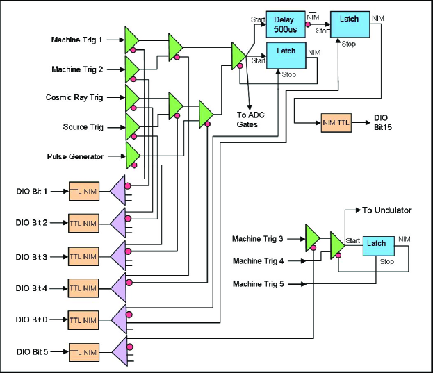
Figure 34: Trigger logic

Trigger Logic:

This hardware subsystem was implemented using NIM electronic modules, and generated the DAQ software trigger, the ADC gates, and the undulator trigger associated either with the SLAC electron beam, or with three types of non-beam events,

Cosmic Ray Trigger, for studying CsI detector performance and calibration.

Radioactive Source Trigger, for diagnostics and calibrations of the CsI detector.

Pulse Generator Trigger.

Triggers associated with the electron beam were based on five signals (Machine Triggers) with different timing relative to the arrival of the beam pulse at the experiment,

Machine Trigger 1 generated a DAQ software trigger and ADC gates in time with the electron beam pulse.

Machine Trigger 2 generated a DAQ software trigger with ADC gates out of time with the electron beam pulse (and was not ordinarily used).

Machine Trigger 3 came 11 $\mu$s before the electron beam pulse to trigger the undulator power supply such that its peak current was in time with the electron beam pulse.

Machine Trigger 4 came 50 $\mu$s after the electron beam pulse to trigger the undulator power supply such that its peak current was out of time with the electron beam pulse.

Machine Trigger 5 came 900 $\mu$s before the electron beam pulse to reset the undulator trigger logic prior to an electron beam pulse.

DIO output bits 1–4 selected the DAQ software trigger and ADC gates to be from one of the three non-beam triggers or Machine Trigger 1 or 2. The NIM logic for this was reset by DIO output bit 0 at the end of the data acquisition for each triggered event. DIO output bit 5 selected the undulator pulse to be in or out of time with respect to the electron beam.

During production data taking the DAQ software trigger and the ADC gates were derived from Machine Trigger 1, while the undulator was pulsed in and out of time with respect to the electron beam on alternate beam pulses by Machine Triggers 3 and 4.

Digitizing Electronics:

Two external bus systems were used:

VME. National Instruments models PCI-MXI-2 and VME-MXI-2 interfaced the VME system to the DAQ computer. The VME crate contained three 8-channel V265 ADC modules from CAEN, one VSAM module from BiRa Systems, one VME-CAN2 module from ESD, and one DVME-626 module from DATEL. The VME-CAN2 module recorded voltage transients induced in the pickup coils upon polarity reversal of the polarimeter magnets TP1 and TP2. The DVME-626 DAC module set the undulator excitation voltage.

GPIB. A National Instruments PCI-GPIB interface was used to drive the GPIB bus. A Kinetic Systems model 3988 CAMAC crate controller interfaced the CAMAC crate to the GPIB bus. The CAMAC crate contained a LeCroy model 2341A Latch Register, three LeCroy model 2249W 11-bit, charge integrating ADCs, and two LeCroy model 2259B 11-bit, peak-sensing ADCs.

3.6.2 DAQ Software

The DAQ software consisted of several programs written with the use of National Instruments LabVIEW version 7.2. These were executed on an Intel Pentium 4 CPU desktop computer operating under Microsoft Windows XP. The activities of these programs were coordinated and they communicated with each other via a set of global variables. Their access to common resources was coordinated using semaphores. One program was coded with the C++ programming language and provided a connection to the SLAC accelerator control system. The software set consisted of the following:

Main DAQ. This program initialized parameters prior to data collection, started, paused, resumed (after a pause) and ended data collection. During data collection it read out the detector data from the digitizing electronics after a trigger, all of which data was written to a disk file and some of which was monitored via various online displays.

High Voltage. This program controlled and periodically monitored the high voltage (HV) subsystem, which powered the silicon detectors GCAL, P1, S1 and S2, the CsI photodiodes, and photomultiplier tubes of the aerogel Cherenkov A1, A2, and other detectors.

Smart Analog Monitor (SAM). This program periodically read a 32-channel VME module to which slowly varying signals were attached, and also displayed and recorded these signals.

Accelerator Control Data Base Monitor. This program transferred various slowly varying parameters from the accelerator control database for online display and recording in a data file. An EPICS-channel-access mechanism implemented retrieval of data from the data base.

Magnet Reversing Control. This program, written in C++, issued requests to the SLAC Accelerator Control System to reverse the polarity of the analyzer magnets.

Several other programs were employed for infrequent control functions and for diagnostic purposes.

3.7 Data Runs

Positron data were collected during two run periods in June and September 2005 at five sets of spectrometer/lens currents (Table 4). Electron data were collected only at one set of spectrometer/lens currents. For each of the spectrometer settings a number of Super runs was taken. One Super run consisted of 10 cycles with 3000 electron beam pulses (events) each at a 10 Hz repetition rate, with the undulator pulse in time with only every other beam pulse. Thus, half of all recorded events were “signal” (undulator in time) and half were “background” (undulator out of time). In an automated procedure the polarity of the positron- and photon-polarimeter magnets TP1 and TP2 was reversed before each cycle by the Magnet Reversing Control program.

The main DAQ program allowed selection of run types from a drop-down menu.

Patterned: In this run type the timing between electron beam pulses and undulator pulses was controlled by a software-coded pattern, usually with the undulator pulsed in time with every other electron-beam pulse.

Pedestal: In this type of run Machine Trigger 1 was used to accumulate a specified number of counts for each ADC channel. However, the electron beam was blocked in the SLAC beam switchyard, upstream of the FFTB, to establish the beam-off state (pedestals) of the data-acquisition system. At the end of a run, the average value was calculated for each channel. These values were used in subsequent runs for subtracting ADC pedestal values in the online displays.

Simple: In this type of run the undulator was pulsed in time with every electron beam pulse.

Special: This run type executed the Magnet Reversing Control program, and also recorded the currents in the polarimeter magnets at 50 Hz via pulse-generator triggers.

Test: This run type allowed manual selection of the trigger source for test purposes.

Super: This run type consisted of a selectable number of cycles, usually 10, where each cycle consisted of a Special run followed by a Patterned run.

3.8 Data-File Structure

Data from each run were written to ASCII disk files. Following a Begin Run record, a string of digitized data from the readout electronics modules was written for each event. The bulk of the data in the file came from the electronic modules digitizing the detector data. In each event string, the detector data were preceded by five words:

1. Data Type Marker - to identify the source of a data string (detectors, high voltage, accelerator data, pedestals, etc.).

2. Run Type - to distinguish among the five run types (other than a Super run) listed above.

3. Event Number - a sequential number labeling consecutive events. This number also identified which cycle within a Super run the data belonged to.

4. Relative Time - the integer time in ms of the event with respect to the run start time. For this it could later be determined if any triggers were missing (not processed) due to the DAQ computer being busy.

5. DIO Register - a 16-bit pattern used to tell which trigger sources were used for the event.

In addition to the detector data, other data strings such as HV data, SAM data, etc., were written to disk asynchronously. Each type of non-detector data string was identified by a distinct Data Type Marker.

4 Simulation

Analysis of the energy dependence of the positron or electron polarization $P_{e\pm}$ from measurements by polarimeter TP1, and predictions for asymmetries in the photon polarimeter TP2, required detailed simulations of the experiment.

The calculation of the analyzing power for positron polarimetry was rather complex, as it had to include simulations of the undulator, the collection- and the spectrometer-system, as well as the polarimeter magnet. These simulations were performed using the Geant4 code [22, 23], starting with version 6.2, which was extended to include all electromagnetic processes needed for spin-dependent transport of particles through matter, as discussed in Sec. 4.1. The spin-dependent extensions are available in Geant4 from version 8.2 [24] onwards.

The simulation procedure for positrons (electrons) was performed in four independent steps, where each subsequent step used the output of the previous one as its input:

• Generation of undulator photons with the appropriate spectrum and polarization, Sec. 4.2.1,

• Conversion of undulator photons to electrons and positrons in the production target T1, Sec. 4.2.2,

• Transport of positrons (electrons) through the magnetic field of the spectrometer D2 to the reconversion target T2, Sec. 4.3,

• Reconversion of positrons (electrons) to photons in the reconversion target T2 and transport of photons (and other particles) through the polarimeter magnet TP1 to the CsI calorimeter, and determination of asymmetry $\delta$ of energy deposition with respect to the magnet polarity, see Sec. 4.4.

The analyzing powers $A_{e^{\pm}}$ were determined from the simulated asymmetries $\delta$ according to the inverse of Eq. (12) for the different spectrometer settings in the experiment.

Simulations relevant to the photon polarimeter TP2 were carried out with a combination of software tools that included semi-analytic calculations, modified versions of Geant3, and parametric modeling. As the undulator radiation provided a broad distribution of photon energies, the calculation of asymmetries required a convolution over energy-dependent detector efficiency, analyzing power, and photon polarization. However, in contrast to the positron case, the transmitted photon beam was narrowly collimated. Thus, it was sufficient to consider only first-generation-scattering events in the iron, which simplified the task considerably, as described in Sec. 4.5.

4.1 Simulation of Polarization in Geant4

The polarization dependence of the following processes has been accounted for in the simulations of the experiment:

• Compton scattering,

• Bhabha and Møller scattering,

• Photoelectric effect,

• Pair creation and annihilation,

• Bremsstrahlung.

Polarization effects were neglected for low-energy charged particles with less than $200\ \mu$m remaining range.

The polarization states of particles are described in Geant4 by Stokes vectors, and polarization transfer from an initial to a final state is represented by a linear transformation of the corresponding Stokes vectors[43]. A detailed description of the implementation of the transfer-matrix formalism for all relevant processes can be found in[25, 61].

4.2 Production of Positrons and Electrons in the Target

4.2.1 Radiation of the Helical Undulator

The photon spectrum of undulator radiation has been discussed in Sec. 2. Table 9

Table 9: Parameters for the simulation of the undulator radiation.

Parameter	Value
Electron beam energy $E_{e}$	46.6 GeV
Undulator period $\lambda_{\rm u}$	2.54 mm
$K$-value	0.19
Energy $E_{1}$ of first harmonic	7.9 MeV
Number of harmonics calculated	3
Total number of photons per $e^{-}$	0.43 m-1
Total radiated power	1.76 MeV/m

summarizes the parameters used for the simulation of the undulator radiation. Only the first three harmonics of the photon spectrum have been included in the simulation. The relative contributions of these harmonics to the total undulator radiation are shown in Table 10;

Table 10: The Fraction $N_{n}/N$ of undulator photons in the first three harmonics and their cutoff energy $E_{n}$ for ${K}=0.19$.

Harmonic number $n$	$N_{n}/N$	$E_{n}$ (MeV)
1	0.9584	7.9
2	0.0396	15.7
3	0.0020	23.5

harmonics higher than the third contributed approximately $10^{-4}$ of the total number of photons in this experiment.

In the simulation of the positron polarimeter the $K$-value of the undulator was assumed to be 10% higher than its design value listed in Table 3 of Sec. 3.2. While this slightly modified the predicted positron and electron rates at high-energy settings of the spectrometer, the impact on the analyzing power, and consequently on the polarization results, was negligible.

4.2.2 Production of Polarized Positrons and Electrons

The photons generated by the undulator were simulated as striking the production target T1 uniformly over a circle 3 mm in diameter, corresponding to the aperture of collimator C2. Although the core of the photon beam was considerably smaller than this (see Sec. 3.1, the position of the beam varied from run to run such that a uniform spatial distribution at collimator C2 was a good approximation. Table 11 lists the parameters used in the Geant4 simulation of the generation of electrons and positrons in the target.

Table 11: Parameters used in the simulation of positron production and transport.

Production
Undulator-photon beam shape	3-mm-diameter cylinder
Production-target material	Tungsten composite W-4Ni-3Cu-3Fe
Production-target thickness	0.81 mm (0.2 r.l.)
Geant4 equiv. energy cutoff	200 $\mu$m remaining path length
Transport through solenoid SL and spectrometer D2
Vacuum-pipe diameter (solenoid)	36 mm
Vacuum (in vacuum chamber)	$10^{-3}$ Torr
Energy-selection slit width	30 mm
Solenoid field map	SLAC measurement
Spectrometer field map	MERMAID calculation
Magnetic field (implementation method)	3-D linear interpolation
Tracking step length (in magnetic field)	100 $\mu$m
Transport from exit window of spectrometer to target T2
Exit-window diameter	48 mm
Reconversion-target material	Tungsten
Reconversion-target thickness	1.75 mm (0.5 r.l.)
Reconversion-target diameter	50 mm
Geant4 equiv. energy cutoff	200 $\mu$m remaining path length

Positrons were produced in target T1 by $\gamma$ conversion to $e^{+}e^{-}$, after which they interacted in the target through Bhabha scttering, annihilation, Bremsstrahlung, ionization, and subsequent cascade processes. Electrons were produced by Compton scattering and the photoelectric effect in addition to pair production. For the conditions of this experiment, the total electron yield at the exit of the target was a factor 2.2 higher than that of positrons: $Y_{e^{+}}^{2\pi}=0.0085$ and $Y_{e^{-}}^{2\pi}=0.0187$ per incident photon. Because of subsequent interactions in the target, these yields were much smaller than the 10.5 % of the primary photons that were converted into electrons and positrons.

Figure 35 shows the simulated energy distributions of electrons and positrons. The expected longitudinal polarization of positrons and electrons at the exit of the production target T1 was essentially the same as that for the same set of particles at the reconversion target T2 (see Sec. 4.4), and the latter is shown in Fig. 41.

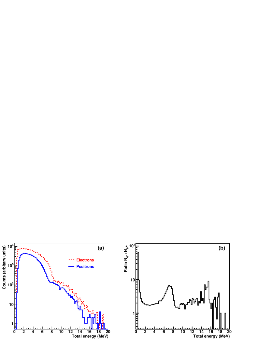
Figure 35: (a) Electron- and positron-energy spectra at the exit face of the production target T1; (b) ratio of electron and positron spectra plotted in (a).

For production by first-harmonic photons (maximum energy $E_{1}=7.9$ MeV), the maximal total energies of the positrons and electrons were

$$E_{e^{+}}^{\rm max} =E_{1}-mc^{2}=7.4\,\mbox{MeV},$$ (18)

$$E_{e^{-}}^{\rm max} =E_{1}+mc^{2}=8.4\,\mbox{MeV},$$ (19)

noting that the maximal-energy electrons were generated by the photoelectric effect. Figure 36

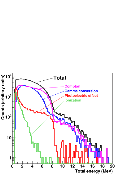
Figure 36: Relative contributions to the energy distribution of electrons from different processes ($\gamma$-conversion, Compton, photoelectric effect and ionization).

shows the energy distribution of the electrons for the different processes; the fractional contributions of the electron-production processes in the production target are given in Table 12.

Table 12: Relative contributions of different processes to the electron production for the parameters in Tables 9 and 11.

Process	Fraction
Compton scattering	0.4987
$\gamma$-Conversion	0.3875
Photoelectric effect	0.0773
Ionization	0.0365

The energy, angular distribution and polarization of the positrons (electrons) at the exit face of the production target were used as input for the next step described in the following section.

4.3 Positron/Electron Transport

4.3.1 Overview

The positrons (electrons) generated in the production target T1 were guided through the transport system by the solenoid lens SL and the spectrometer dipoles D2 (Sec. 3.5.2, Figs. 3, 11 and 20) while the oppositely charged particles – the electrons (positrons) – were dumped.

The simulation of the transport system and the tracking of the polarized positrons (electrons) yielded the following output for each set of currents $(I_{\rm S},I_{\rm L})$:

• Positron/electron transmission through the spectrometer system,

• Positron/electron energy and spatial distributions at the Si-W detector P1 and at the reconversion target T2.

The distributions at the reconversion target T2 constituted the input for the simulation of measurements by the positron polarimeter described in Section 4.4. Depolarization effects due to spin precession in the magnetic field [64] were negligible in the present experiment, and have been ignored in the simulation.

4.3.2 Implementation of the Magnetic Fields

Solenoid Magnetic Field:

The magnetic field of the focusing lens SL was implemented in the simulation using the functional forms (13)–(15) and the measured values of $B_{0}(z)$. The focusing effect is illustrated in Fig. 37.

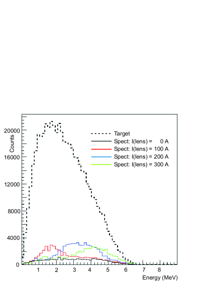
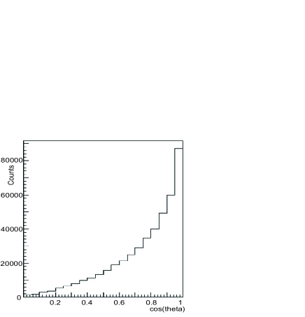
Figure 37: Simulations of focusing of positrons by the solenoid lens SL. Left: The energy spectra of positrons emerging from the production target T1 and of positrons entering the spectrometer D2 for different solenoid currents. Right: The polar angle distribution, $\cos\theta$, of positrons at the target exit surface.

For each spectrometer current $I_{\rm S}$ the solenoid current $I_{\rm L}$ used in the simulation was chosen to maximize the number of positrons at the detector P1. Because the field map used in the simulation differed somewhat from the actual field in the solenoid, the currents $I_{\rm L}$ used in the simulation differed slightly from those used in the experiment, as shown in Table 4, but the focusing effect of the solenoid lens was thereby well represented in the simulation.

Spectrometer Magnetic Field:

In the simulation, the MERMAID field map described in Section 3.5.2 was implemented using a three-dimensional linear interpolation on a cubic grid. The magnitude of the field was related to the spectrometer current $I_{\rm S}$ according to Eq. (17).

4.3.3 Energy Selection by the Spectrometer

The spectra of positron energies at the reconversion target T2 as selected by the movable tungsten jaws J in spectrometer D2 was simulated for the five spectrometer currents $I_{\rm S}$, as shown in Fig. 38.

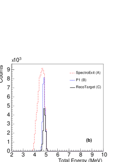
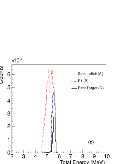
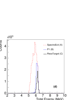
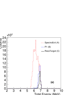
Figure 38: Simulated positron-energy spectra at the exit of the spectrometer (position A of Fig. 20), at the detector P1 (position B), and at the reconversion target T2 (position C) for the five spectrometer currents, (a): $I_{\rm S}=100$  A, (b): $I_{\rm S}=120$  A, (c): $I_{\rm S}=140$  A, (d): $I_{\rm S}=160$  A, (e): $I_{\rm S}=180$  A.

While the efficiency of the positron transport was sensitive to the current $I_{\rm L}$ in the solenoid lens, the shape of the transported energy spectra depended only slightly on this current. The resulting dependence on spectrometer current of the central energies of positrons transported to the reconversion target T2 is listed in Table 4.

4.3.4 Positron Transport Near Detector P1

As discussed in Sec. 3.5.2 the vacuum chamber was inadvertently constructed with the exit port 6.3 mm further away from the $\gamma$-line than called for in the magnet design. Moreover, the presence of unsuspected magnetism of the tungsten that faced the iron pole pieces led to a deviation of the positron paths from their design trajectories. In consequence the emergent beam from the vacuum chamber was not centered on the axis of the polarimeter magnet. The energy selection resulted from a combination of the jaws setting and the aperture of the spectrometer exit tube.

The horizontal asymmetry of the positron distribution at detector P1 (Sec. 3.5.3) was confirmed qualitatively by simulations shown in Fig. 39, where ideally the positrons would be centered on $x=0$ at the spectrometer exit (curve A), at the detector P1 (curve B) and at the reconversion target T2 (curve C); see also [61].

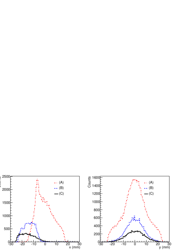
Figure 39: Simulated distributions of positrons along the $x$- and $y$-axis at the exit of the spectrometer D2 (A), at the detector P1 (B) and at the reconversion target T2 (C) for spectrometer current 140 A.

4.4 The Positron Polarimeter

Positrons that struck target T2 were reconverted into photons, some of which passed through the iron-core polarimeter magnet TP1 and were absorbed in the CsI(Tl) calorimeter, as described in Sec. 3.5. The flux of photons in the calorimeter depended on the polarization of the positrons (as well as that of the electrons in the magnet iron). The spatial, momentum and polarization distributions of positrons at the reconversion target from the preceding simulations were the input for the simulation of the positron polarimeter.

4.4.1 The Analyzing Power

By reversing the polarity of magnet TP1 an asymmetry $\delta$, defined in Eq. (8), in the energies observed in the nine CsI crystals was obtained. The analyzing power $A_{e^{\pm}}$ for positron (electron) polarization is given by

$$A_{e^{\pm}}=\frac{\delta}{P_{e^{\pm}}P_{e^{-}}^{\rm Fe}}~{}~{},$$ (20)

where $P_{e^{\pm}}$ and $P_{e^{-}}^{\rm Fe}\ (=0.069\pm 0.002)$ are the positron (electron) longitudinal polarization and the polarization of the electrons in iron, respectively. To improve the statistical significance of the simulation, the positron polarization as well as the absolute polarization of the iron absorber were set to 100 % and the results scaled to the actual polarization values. The results are shown in Fig. 40

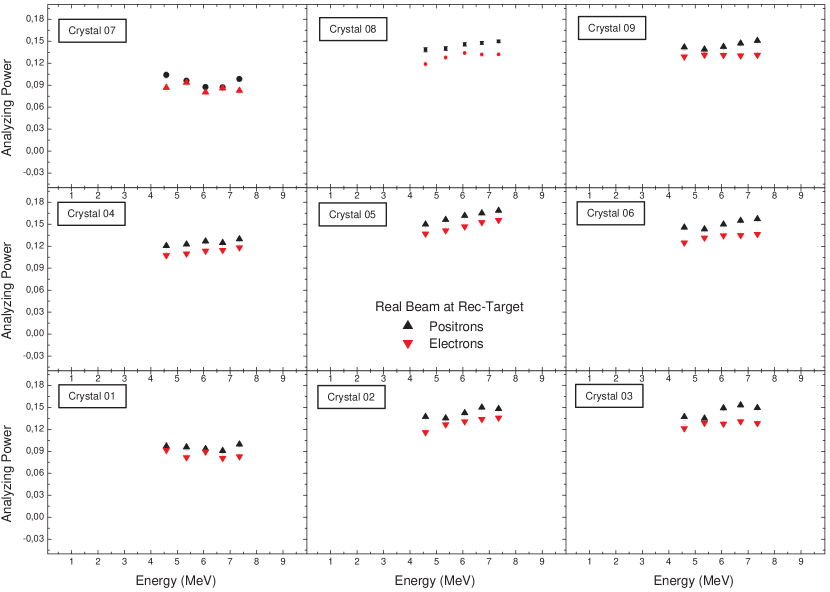
Figure 40: The simulated analyzing power $A_{e^{\pm}}$ of each of the nine CsI crystals for positron and electron polarization.

as a function of electron and positron energy. The analyzing power differed slightly for the individual crystals in the CsI(Tl) calorimeter, due to their different geometrical acceptance. The analyzing power for the central crystal is listed in Table 13 for the various spectrometer current settings; the uncertainties were due to limited statistics in the simulation.

Table 13: The analyzing powers $A_{e^{\pm}}$ for electrons and positrons in the central CsI crystal at different spectrometer currents $I_{\rm S}$.

$I_{\rm S}$ (A)	E${}_{e^{\pm}}$ (MeV)	$A_{e^{+}}\pm\Delta A_{e^{+}}$	$A_{e^{-}}\pm\Delta A_{e^{-}}$
100	4.59	$0.1498\pm 0.0016$	$0.1371\pm 0.0018$
120	5.36	$0.1563\pm 0.0015$	$0.1417\pm 0.0016$
140	6.07	$0.1616\pm 0.0014$	$0.1469\pm 0.0015$
160	6.72	$0.1651\pm 0.0013$	$0.1528\pm 0.0014$
180	7.35	$0.1686\pm 0.0013$	$0.1557\pm 0.0014$

The systematic uncertainty on the simulation of the analyzing power was estimated to 7 % by varying the Geant4 physics parameters within their allowed range.

4.4.2 The Asymmetries $\delta$ and the Polarizations $P$

The asymmetries $\delta$ in the energies observed in the crystals of the CsI calorimeter on reversal of the polarity of magnet TP1 was predicted from the simulated polarization $P_{e^{\pm}}$ of positrons (electrons) after the production target (see Sec. 4.2) and the analyzing power $A_{e^{\pm}}$,

$$\delta=A_{e^{\pm}}P_{e^{\pm}}P_{e^{-}}^{\rm Fe}~{}~{}.$$ (21)

Figure 41 shows the simulated polarization of positrons (electrons) after the production target, together with the analyzing power in the energy range 2.0–9.5 MeV. The asymmetries $\delta$ expected in the central CsI crystal are shown in Fig. 42, where the results of a simulation of an ideal pencil-like beam are also presented.

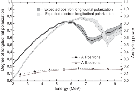
Figure 41: The simulated polarization $P_{e^{\pm}}$ of positrons/electrons at target T2 and the respective analyzing powers $A_{e^{\pm}}$ in the central CsI crystal as a function of particle energy.

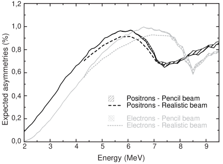
Figure 42: Simulations of the asymmetries $\delta$, Eq. (8), of the energies observed in the central CsI crystal on reversal of the polarity of magnet TP1 as a function of positron/electron energy for the experimental beam and for a pencil beam.

4.5 The $\gamma$-Line

4.5.1 Photon Spectra

The simulation of the $\gamma$-line was carried out with two special simulation tools based on Geant3, as modified to include polarization-dependent absorption cross sections. The first of these generated the undulator-photon spectrum through third order in the undulator-strength-parameter $K$, and corrected the spectrum for absorption in the production target T1, the incident-flux detectors A1 and S1, the magnetized-iron polarimeter TP2, and the transmitted-flux detectors A2, S2, and GCAL. The code allowed separate examination of contributions from Compton scattering, pair production, and the photoelectric effect. It also incorporated the response functions discussed in Sec. 4.5.2 to calculate the signal generated in each detector by the passage of the photon beam. The program did not treat effects of beam divergence or collimator acceptance.

Figure 43

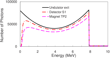
Figure 43: Simulated photon spectra $N_{\gamma}(E)$ at the exit of the undulator, at detector S1, and incident on polarimeter magnet TP2.

shows photon spectra $N_{\gamma}(E)$ as simulated by this program at the exit of the undulator, at detector S1, and incident on the polarimeter magnet TP2, assuming a first-order cutoff energy of $E_{1}\approx$ 7.9 MeV ($K\approx 0.17$) and that the production target T1 was 0.81 mm of tungsten alloy. The loss of photons at very low energies (and large angles) in the first simulation was due to absorption in the production target T1, which also removed 10 % of photons of all higher energies. Another 16 % of the photons were absorbed in the 0.5-mm-thick tungsten convertor of detector S1 and in 1 cm of aluminum in detector A1 before the beam reached magnet TP2. Figure 44

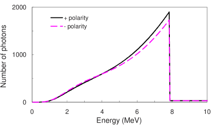
Figure 44: Simulated spectra $N_{\gamma}(E)$ of photons at detector S2 for both polarities of magnet TP2.

shows the predicted photon spectrum at counter S2 behind polarimeter magnet TP2 for both states of polarization of the iron, assuming electron polarization $P^{\rm Fe}_{e^{-}}=7.23$ % (Table 6). The magnet iron reduced the photon flux by a factor of $\approx 50$. The relative number of photons and the relative total energy in the photon beam at various components along the $\gamma$-line are summarized in Table 14; not included are possible losses in collimators C2-C4.

Table 14: Results of a Geant3 simulation of the relative number of photons, their relative total energy, and the average energy per photon at the upstream face (except as noted) of various $\gamma$-line components. In this simulation the photon beam incident on target T1 was the same as that at the exit of the undulator. Beyond TP2 results are reported for both polarities of that magnet.

Component	Photon	Total	$\langle$Energy$\rangle$ per
	number	energy	photon (MeV)
Target T1	1.000	1.000	4.116
Exit of T1	0.895	0.939	4.316
Detector S1	0.881	0.927	4.332
Detector A1	0.835	0.888	4.380
Magnet TP2	0.739	0.807	4.494
Detector A2 $(+)$	0.01406	0.02010	5.885
A2 $(-)$	0.01334	0.01880	5.802
Detector S2 $(+)$	0.01280	0.01840	5.912
S2 $(-)$	0.01214	0.01720	5.831
Detector GCAL $(+)$	0.01229	0.01765	5.909
GCAL $(-)$	0.01165	0.01650	5.828

The second simulation tool folded the beam emittance with the undulator spectrum to examine the geometric transmission of the photon beam through the aperture of collimator C2. It could independently vary the size of the C2 aperture, the lateral displacement, and the angle of the collimator axis with respect to the axis of the photon beam. For example, Fig. 45 shows the C2 acceptance of undulator photons ($N_{\rm transmitted}/N_{\rm incident}$) as a function of collimator aperture when the beam axis and collimator axis coincide. The nominal diameter of that collimator was 3 mm, so that 93 % of the photons, and 98.9 % of their energy, passed through the collimator if the beam was properly aligned. Because of the correlation (4) between photon energy and angle, the photons that were absorbed by the collimator had very low energy. Lateral displacement of the photon beam had a relatively small effect on the C2 acceptance if the collimator axis was parallel to the beam axis; a 1 mm displacement resulted in a loss of acceptance of 10 %. The simulation also showed that for a 5 mrad tilt of the C2 axis with respect to the beam axis the loss of acceptance would be only 3 %, but a combination of the tilt plus a 1 mm displacement of the axes could cause reduction in acceptance of up to 48 %, in which case S1 and PRT would only cover a corresponding fraction of the full undulator-photon flux.

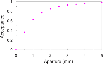
Figure 45: Simulated acceptance of the collimator C2 as a function of the collimator aperture, assuming that the photon beam axis and the collimator axis coincided.

4.5.2 $\gamma$-Detector Response

Figure 46 shows the results of the Geant3 simulation of energy deposition $R(E)$ in various Si-W detectors as a function of the energy $E$ of single incident photons.

Figure 46: Geant3 simulation of the single-photon response $R(E)$ of the $\gamma$-detectors S1/S2, GCAL, and PRT.

Estimates of the detector sensitivities (in ADC counts, Sec. 3.4.2) were obtained by convoluting the single-photon response $R(E)$ of the detectors with the corresponding spectrum $N_{\gamma}(E)$ of incident photons (Sec. 4.5.1).

Without attenuation, the average sensitivity of detector S1 for the photon spectrum labeled S1 in Fig. 43 would have been approximately 1250 photons per ADC count, corresponding to 1420 photons at the exit of the undulator. It was therefore necessary for normal data acquisition to attenuate the signal by a factor of 199.5 (46 dB), such that one ADC count for S1 corresponded to 283,000 photons.

Although detectors S1 and S2 were identical in construction, the energy spectra of incident particles were quite different and the unattenuated sensitivity of S2 was about 950 photons/ADC count; and that of GCAL about 135 photons/ADC count. In the experiment the S2 signal was attenuated by a factor of 10 (20 dB) and that of GCAL by 100 (40 dB). For the PRT detectors, assuming that the incident spectrum was an undisturbed undulator spectrum, the sensitivity was 860 photons/ADC count and the attenuation used was 316.2 (50 dB). For the PCAL detectors, which monitored positrons of GeV energy, the unattenuated sensitivity was about 600 MeV/ADC count. The attenuation was 40, 50, and 70 dB for PCALc, PCALd, and PCALe, respectively. The A1 and A2 Cherenkov counter sensitivities were obtained by comparison with the S1 and S2 signals shown in Fig. 19.

4.5.3 Transmission Ratios and Asymmetries

The first Geant3 simulation (Sec. 4.5.1), which included the response functions $R(E)$ for detectors S1, S2, and GCAL and the corresponding spectra $N_{\gamma}(E)$ of incident photons, was used to calculate the signal transmission ratios S2/S1 and GCAL/S1 for both polarities of polarimeter magnet TP2, and the transmission asymmetries $\delta$ of Eq. (8), as shown in Table 15.

Table 15: Simulations of the transmission of photons from the undulator though detectors S2 and GCAL, normalized to the photon flux at detector S1, and of the signal asymmetries with respect to the polarity of magnet TP2 in detectors A2, S2, and GCAL.

Detector	Transmission
S2$(+)$/S1	0.0202
S2$(-)$/S1	0.0189
Average	0.0195
GCAL$(+)$/S1	0.1366
GCAL$(-)$/S1	0.1274
Average	0.1320
	Asymmetry
A2	0.0363
S2	0.0339
GCAL	0.0347

A reliable calibration was obtained for the absolute response of the silicon detectors, but not for the Cherenkov detectors, so simulation of transmission ratios was possible only for S2 and GCAL relative to S1. For detector A2 only the transmission asymmetry $\delta$ was simulated, assuming a Cherenkov cutoff of 3.8 MeV and a response proportional to $1-1/n^{2}\beta^{2}$ above threshold.

5 Background Studies

Two classes of backgrounds were studied: those associated with the primary electron beam; and those associated with energizing the undulator.

5.1 Backgrounds Related to the Primary Electron Beam

Backgrounds associated with the primary electron beam were due to secondary particles that reached various detectors from electromagnetic showers of particles in the tails of the primary beam, as well as due to backsplash from the interaction of the primary beam with the dump at the end of the FFTB. These backgrounds were mitigated by protection collimators prior to the last “dogleg” bend in the FFTB, and by extensive lead shielding between the experimental detectors and undulator, and also between the detectors and the beam dump.

The major source of electron-beam-related backgrounds was interaction of the tails of the beam with the protection collimator C1 (0.71 mm in aperture and 6.35 cm long; see Sec. 3.1) and with undulator bore tube (0.9 mm in aperture and 1 m long). This was confirmed by comparison of rates in normal data runs with those in occasional runs with collimator C1 and the undulator moved out of the electron beam and a 2.5-cm-diameter bypass vacuum pipe inserted in the beam using an articulated mover, sketched in Fig. 11. Table 16 compares the responses of various detectors, normalized to a beam intensity of $3\cdot 10^{9}\,e^{-}$/pulse, for two such runs.

Table 16: Comparison of rates in ADC counts for the signals (after correction for attenuation) in various detectors for two runs, No. 1702 with undulator out, and No. 2803-5 with the undulator inserted but energized out of time with the electron beam.

Detector	Undulator	Undulator in
	removed	but out of time
A1	0.7	81.6
A2	0.2	61.2
CsI	11.6	71.3
GCAL	17.9	16725.2
P1	0.1	-0.2
PCALc	-0.1	7287.3
PCALd	-0.4	17590.2
PCALe	0.0	24740.4
PRTleft	1.2	23171.0
PRTright	-10.4	3308.4
PRTtop	47.5	7807.4
PRTbottom	-5.5	3962.2
S1	35.5	1178.6
S2	0.1	425.1

In the absence of the undulator, the rates were small and we were unable to ascertain the relative contribution from interactions of the electron beam with material upstream and downstream of the location of the undulator. In particular, the level of background due to backsplash from the electron beam dump was very small and no correction was made for it in the data analysis.

When the undulator was in place, but not energized in time with the electron beam, the rates increased slightly in the two detectors of the positron polarimeter, CsI and P1, which were displaced by 464 mm from the $\gamma$-line. In contrast, the rates in detectors along the $\gamma$-line (including the PCAL) increased by factors of several hundred when the undulator was introduced.

Secondary photons from interactions of the tails of the electron beam with the undulator followed a path similar to undulator-generated photons and were the main source of background rates in the various $\gamma$-line detectors. Secondary electrons from interactions in the undulator (or material upstream thereof) were deflected downward by the dump magnet string D1 (Fig. 2) and were largely absorbed in the magnet yokes or in the lead shielding (shown in Fig. 11) upstream of the detectors. Secondary positrons were deflected upwards and could have created minor backgrounds in the $\gamma$-line detectors via tertiary particles from interactions with the ceiling of the FFTB tunnel; this may have been the major source of background in the CsI detector.

The large rates in detectors S2 and GCAL downstream of polarimeter magnet TP2 were due to low-energy particles from showers of high-energy background photons in the magnet iron. These low-energy particles were not observed in Cherenkov counter A2 which threshold was about 4 MeV.

The energy observed in the PCAL detectors was largely due to high-energy positrons from interactions of primary electrons with collimator C1 and the undulator bore tube. From this energy it was estimated that only about one beam particle in $10^{5}$ so interacted.

During normal data collection, backgrounds associated with the tails of the primary electron beam were separated from signals due to undulator photons by energizing the undulator in- and out-of-time with respect to the electron beam on alternate pulses. Table 17 shows the average background and undulator-photon signal (undulator-on minus undulator-off) in various detectors for a sample of 211 runs during September 2005.

Table 17: Background and signal ADC counts in various detectors for a sample of September 2005 runs. The background is from undulator-off data and the signal is undulator-on minus undulator-off.

Detector	Background	Signal	Signal/Background
A1	242.3	543.7	2.4
A2	210.7	13.7	0.1
CsI	136.0	29.0	0.2
GCAL	580.5	91.0	0.2
P1	9.3	509.2	54.9
PCALe	30.9	-1.4	-0.1
PRTtop	59.8	259.8	4.3
PRTright	27.5	229.1	8.3
PRTbottom	29.9	292.3	9.8
PRTleft	159.9	598.2	3.7
S1	5.8	164.4	28.5
S2	169.5	95.5	0.6

The signal-to-background ratios were different for the central crystal (CC), the four crystals touching the central one along a side (NC = nearest crystal), and the four crystals in the corners (DC = distant crystal). The undulator-off signal levels were typically about 66 %, 84 %, and 91 % of those for CC, NC, and DC in undulator-on events, respectively. The average energy deposition per beam pulse for undulator-off events in the central crystal, for example, varied between 130 and 280 MeV, such that the signal (undulator-on $-$ undulator off) to background (undulator-off) ratio varied between 0.2 and 1.2.

Details of the background subtraction in the positron analysis will be presented in Sec. 7.3.

5.2 Undulator-On Backgrounds

Background in the CsI detector associated with energizing the undulator principally were due to secondary particles from interactions of undulator photons with collimators, beam windows, and target T1 which reached the detector by other than the nominal path through the positron spectrometer D2. In addition, the small deflection of the primary electron beam by the undulator, discussed in Sec. 3.2.3, might have changed the level of backgrounds associated with interaction of tails of the primary electron beam with the undulator body.

A measure of the undulator-induced backgrounds in the central CsI crystal was obtained in a set of runs during September 2005 in which target T1 was removed, and data collected, as usual, with the undulator both on (in time with the electron beam) and off (out of time), as shown in Fig. 47. The average target-out, undulator on-off difference was 4.2 ADC counts out of the typical background level of 100 ADC counts due to effects of the primary electron beam.

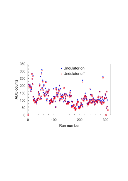
Figure 47: CsI-central-crystal signal in ADC counts for all September 2005 runs with positron target T1 removed and undulator on (circle) or off (rhombus).

Additional evidence for a small change of the interaction of the tails of the primary electron beam with the undulator due to energizing the undulator was obtained from the PCAL detectors. For example, PCALc and PCALe consistently recorded an undulator-on/off ratio of $(95.5\pm 0.5)\,\%$, as shown in Fig. 48, while PCALd gave a ratio of $(100.0\pm 0.5)\,\%$.

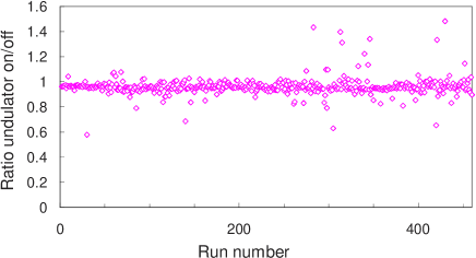
Figure 48: Ratio of energies for undulator-on/off measured by detector PCALe for a series of runs.

No correction was made for this small difference between undulator-on and undulator-off background, but it was included as a term in the estimate of the systematic uncertainty of the positron polarization (Sec. 7.5).

6 Photon Analysis

6.1 Undulator Performance

6.1.1 Photon Beam Intensity

Based on the design parameters of the undulator, as described in Secs. 2.1 and 3.2, the undulator generated 0.35 photons per beam electron with angle-energy distribution (4). Thus, half of the photons were emitted at angles larger than $1.1\,\mu$rad to the direction of the electron beam, such that the flux observed in the $\gamma$-detector S1 was strongly influenced by the alignment of the primary electron beam. During the experiment, the electron beam was steered to minimize backgrounds generated by interactions with collimator C1 upstream of the undulator, rather than to maintain optimal alignment of the $\gamma$-beam. To include a measure of the phtoton flux outside collimator C1, photon intensity measurements were based on the sum of signals in detector S1 and in the quadrant detector PRT that observed photons outside the aperture of collimator C2.

Figure 49

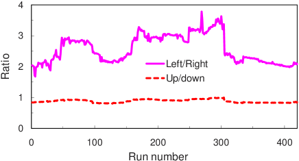
Figure 49: The left/right and the up/down ratios measured in the PRT quadrant detectors during 420 runs.

shows the left/right and up/down ratios of rates in the four PRT $\gamma$-detectors for 420 runs at spectrometer current $I_{\rm S}=100$ A. The beam displacement at collimator C2 was primarily in the $x$ (horizontal) direction, and the observed left/right ratios corresponded to displacements from 500 to 1100 $\mu$m according to simulations. The average $y$ (vertical) displacement was less than 100 $\mu$m. The anticorrelation of the signals in detectors PRT and S1 is shown in Fig. 50 for the same set of runs as in Fig. 49.

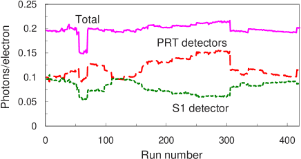
Figure 50: Undulator photons per beam electron in the PRT and S1 detectors for the same 420 runs as in Fig. 49.

The sum of the signals in the PRT and S1 detectors remained fairly constant at about 0.2 photons per electron. Averaged over the entire experiment, the rate of undulator photons observed in the PRT and S1 detectors per beam electron was 0.199$\pm$0.008, about 60 % of the design performance.

6.1.2 Intensity and $K$-Value vs. Undulator Current

The undulator $K$-value (1) depended linearly on the excitation current of the undulator, while the photon intensity (2) varied as the square of $K$-value, and hence as the square of the current. Several scans of photon intensity vs. undulator current were conducted during the experiment. Results from one of these scans, shown in Fig. 51,

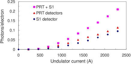
Figure 51: Photons per beam electron in the PRT and S1 detectors vs. undulator current.

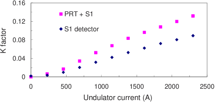
Figure 52: Dependence of the $K$-value on the undulator current as determined from the number of photons per beam electron observed in the PRT and S1 detectors.

exhibit the expected quadratic dependence of intensity on current. The observed photon intensities in detectors PRT and S1 were converted to estimates of the $K$-value via Eq. (2), with results shown in Fig. 52. The estimated $K$-value varied approximately linearly with current, but was below the design value of 0.17 at 2300 A. The discrepancy can be explained by the observed misalignment between collimator C2 and the photon beam, as discussed in Sec. 4.5.1.

6.1.3 Effect of Ferrofluid in the Undulator

Near the end of the experiment the cooling oil in the undulator was replaced by Ferrofluid EMG 900, as discussed in Section 3.2. The increase in undulator magnetic field resulted in an increase of the photon flux by 10–12 %, as shown in Fig. 53.

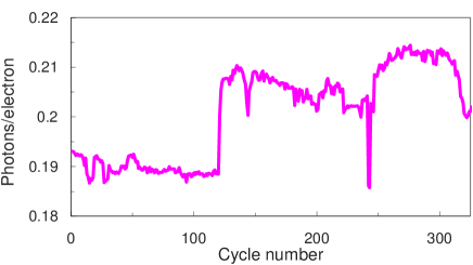
Figure 53: Photons observed in the PRT and S1 detectors per beam electron during operation with spectrometer current $I_{\rm S}=180$ A. Ferrofluid was used in the undulator beginning with cycle 132.

6.2 Photon Transmission through Magnet TP2

Measurements of the transmission of undulator photons through the magnetized iron of the polarimeter magnet TP2 were made by comparing rates in detectors GCAL and S2 to those in detector S1. Detector A2 was not used for this measurement as its signal normalization was not well determined.

Two rather small samples of data from the June 2005 provided the most reliable direct transmission measurements, as shown in Fig. 54.

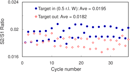
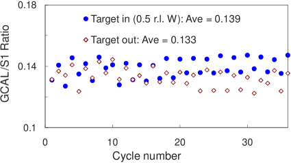
Figure 54: Transmission of undulator photons through magnet TP2 as measured with detectors S2 (left) and GCAL (right), both normalized to detector S1.

One set of data was taken with the target removed and the other with the 0.5 r.l. tungsten target. The variation in rate with alternating cycles was due to the reversal of polarity of magnet TP2. The transmission ratios S2/S1 and GCAL/S1 are given in Table 18

Table 18: The transmission ratios S2/S1 and GCAL/S1 averaged over the run cycles shown in Fig. 54, and a comparison with a Geant4 simulation.

	Target out	0.5 r.l. Target	0.2 r.l. Target
			(simulation)
S2/S1	0.0182	0.0194	0.0195
GCAL/S1	0.133	0.139	0.132

along with a comparison with a simulations described in Sec. 4.5.3. The agreement with predictions is reasonable given the intrinsic uncertainty in unmeasured undulator parameters and beam conditions. Qualitatively, the measured transmission is greater with the target in place as the target hardens the spectrum resulting in increased penetration of the iron absorber.

During data collection in September 2005 collimator C4 downstream of magnet TP2 was inadvertently displaced so as to intercept a portion of the transmitted photon beam, resulting in a loss of about half of the transmitted signal. While this did not interfere appreciably with the measurement of photon polarization (Sec. 6.3), it resulted in unreliable transmission measurements.

Gradual drifts with time of the transmissions measured by both S2 and GCAL were observed, as shown in Fig. 55. The source of this drift with run conditions has not been clearly identified, but it may have been due to changes in beam alignment relative to collimators C2–C4 that altered the energy spectrum of the photons in the $\gamma$-line.

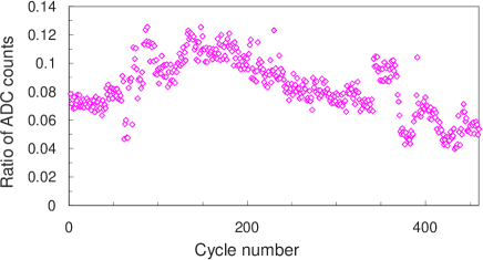
Figure 55: Ratio of the signal in detector S2 to that in S1 for a set of cycles with spectrometer current $I_{\rm S}=140\,A$.

6.3 Photon Transmission Asymmetry

The transmission asymmetry $\delta$, defined in Eq. (8), was measured with each of the three detectors S2, A2, and GCAL (in sequence along the $\gamma$-line).

The data shown in Fig. 54 illustrate the dependence of the rate of transmission of photons through the iron-core magnet TP2 on the polarity of its field. The transmission asymmetries observed in detectors A2, GCAL, and S2 between adjacent cycles (with reversal of the polarity of magnet TP2 on alternate cycles) during a sequence of 420 cycles during 42 Super runs (Sec. 3.7) are shown in Fig. 56.

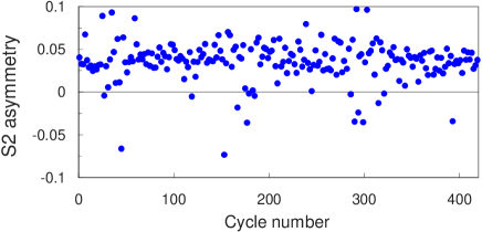
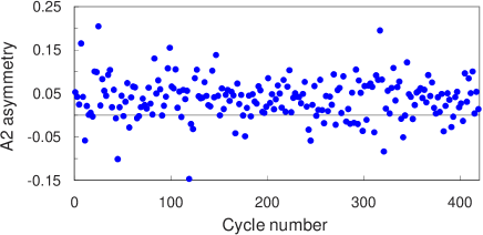
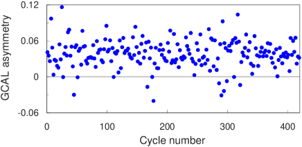
Figure 56: The asymmetries $\delta$ observed between adjacent cycles in detectors S2, A2, and GCAL during 420 cycles with spectrometer current $I_{\rm S}=100\,A$.

Average backgrounds were subtracted on a run-by-run basis. Runs with unstable beam conditions were eliminated by visual inspection of a standard set of plots, and noisy single events were removed by cuts on background detectors. Data for individual runs were normalized to incident photon intensity observed in detector S1. This normalization was superior to that based on the electron beam current as the former included effects of undulator fluctuations and of steering of the photon beam through collimator C2. Normalization to aerogel detector A1 gave similar results.

Figure 57

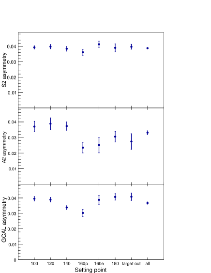
Figure 57: The average asymmetry $\delta$ observed in the photon detectors S1, A1, and GCAL in the seven data segments (Table 4) of the experiment, as well as the asymmetries averaged over the entire experiment.

shows the averaged asymmetries observed in the three detectors during seven positron-data segments (Table 4), as well as the overall asymmetries. Typically, a single data segment consisted of a few hundred cycles from 30–50 Super runs. The smallest uncertainties were obtained with detectors S2 and GCAL; this was not due to an intrinsic limitation of the aerogel detector A2 but rather to insufficient attention to its PMT gain during data collection. The variation of the asymmetries observed in S2, A2, and GCAL with spectrometer current was not predicted and is not understood.

Table 19

Table 19: Measured and predicted asymmetries $\delta$ of signals in the $\gamma$-detectors on reversal of the polarity of magnet TP2, averaged over the entire experiment. The uncertainties are statistical.

Detector	Asymmetry
	Measured	Predicted
A2	0.0331 $\pm$ 0.0012	0.0363
GCAL	0.0367 $\pm$ 0.0007	0.0347
S2	0.0388 $\pm$ 0.0006	0.0339

shows the average measured and predicted asymmetry for each detector for the entire run. The uncertainties listed are purely statistical. The good agreement between the measured and simulated asymmetries indicates that the undulator produced the expected spectrum of photon polarization.

7 Positron Polarization Analysis

The longitudinal positron polarization $P_{e^{+}}$ was derived from the asymmetry $\delta$, introduced in Secs. 2.3–2.4, of the energy deposition $E^{\pm}$ in the CsI calorimeter with respect to the two polarization states (+ and $-$) of the iron-core magnet TP1,

$$\delta=\frac{E^{-}-E^{+}}{E^{-}+E^{+}}=A_{e^{+}}P_{e^{-}}^{\rm Fe}P_{e^{+}},$$ (22)

where the (positive) analyzing power $A_{e^{+}}$ was obtained from the simulations described in Sec. 4.4.1, and the average longitudinal polarization $P_{e^{-}}^{\rm Fe}$ of atomic electrons in the magnet iron was determined to be $0.0695\pm 0.0015$ for $r\leq 22.5$ mm (Table 7). The CsI energy signals $E^{\pm}$ were corrected for background and normalized to the number of positrons observed in detector P1 at the exit of the spectrometer D2, as discussed below.

The best results, in terms of highest signal-to-background ratio and least systematic uncertainty, were obtained using only the central CsI crystal, and only the analysis of the data from that crystal is described here. See [65] for details of the analysis of the other nine crystals.

7.1 General Analysis Procedure

The steps in the positron polarization analysis were:

• Energy calibration of the signals in the CsI crystals (Sec. 3.5.6).

• Selection of events for each positron-energy setting that were recorded under stable beam and background conditions (Sec. 7.2). The data structure has been described in Sec. 3.7.

• Subtraction of the background for every undulator-on event in each CsI crystal, and normalization of the signals in the calorimeter for each event to the number of positrons observed in detector P1 (Sec. 7.3).

• Determination of the asymmetry at each positron energy from a fit to the asymmetries between pairs of adjacent cycles (Sec. 7.4).

• Evaluation of systematic uncertainties in the asymmetry/polarization measurements (Sec. 7.5).

• Comparison of the asymmetries with simulation (Sec. 7.6).

• Calculation of the positron (electron) polarizations from the asymmetries observed in the central CsI crystal (Sec. 7.7).

7.2 Data Selection

There were six spectrometer/lens settings for positron data (see Table 20), and a test was made with the undulator filled with ferrofluid at the highest-current setting. Electron data were taken at only one spectrometer setting, $I_{\rm S}=160$ A. The two data sets at $I_{\rm S}=140$ A were taken at the beginning and at the end of the second run period in September 2005, respectively. The data set with $I_{\rm S}=150$ A was recorded during June 2005 and, unlike the other data sets, its cycles were not combined into runs. Instead, every cycle was recorded individually and the polarity of magnet TP1 was reversed manually in between. Since detector P1 did not exist in the first running period, these data could not be normalized to the positron flux and do not enter in the final results.

Table 20: Event samples (data segments) at various spectrometer settings, together with the corresponding numbers of events before and after the beam-current cuts described in the text, and the fraction $\eta$ of events which were used to determine the average asymmetries of the crystal signals. $I_{\rm S}$ is the current in spectrometer magnet D2 which defined the positron (electron) energy. The label “ff” indicates the data set for which the undulator was run with ferrofluid.

IS	$E_{e^{\pm}}$	Particle	Number of	Number of Events ($\cdot 10^{3}$)			$\eta$
(A)	(MeV)	type	cycle pairs	Before cuts	After cuts	Used in fits
100	4.59	e+	207	1240	1202	958	0.800
120	5.36	e+	187	1119	1082	867	0.804
140	6.07	e+(1)	283	1422	1368	1057	0.787
140	6.07	e+(2)	220	1320	1280	1015	0.795
150	6.41	e+	51	224	215	169	0.791
160	6.72	e+	169	1014	983	767	0.781
160	6.72	e-	145	870	846	676	0.801
180	7.35	e+	65	390	380	294	0.776
180	7.35	e+(ff)	104	624	601	481	0.803
$\sum$			1431	8223	7957	6284

In all steps of the analysis adjacent cycle pairs were treated in parallel. For example, both cycles of a pair should have similar and stable beam and background conditions. To assure stable beam conditions, only those events from both cycles were selected that had a beam-current value, measured by toroid BT (see Fig. 2), within $\pm 3\sigma$ of the mean of that value during both cycles, as illustrated in Fig. 58. That example is not typical; in most cases the beam-current distribution was Gaussian with a $\sigma$ of 2-3 % about the mean.

Figure 58: Example of a distribution of the beam current in toroid BT (see Fig. 2) that shows a fluctuation to low current. Only events with current within the $\pm 3\sigma$ cuts about the mean were used in the subsequent analysis.

7.3 Background Subtraction, Normalization, and Energy Deposition in the Crystal

As discussed in Sec. 5.1, backgrounds in the CsI crystals due to interactions of primary beam electrons were monitored by operation of the undulator out of time with the electron beam (“undulator off”) during alternate beam pulses. Figure 59 gives examples of energies observed in the central CsI crystal during undulator-on and -off events. The variation in the relative amount of background in different CsI crystals required determination of the asymmetries and polarizations, and their corresponding uncertainties, separately for each crystal.

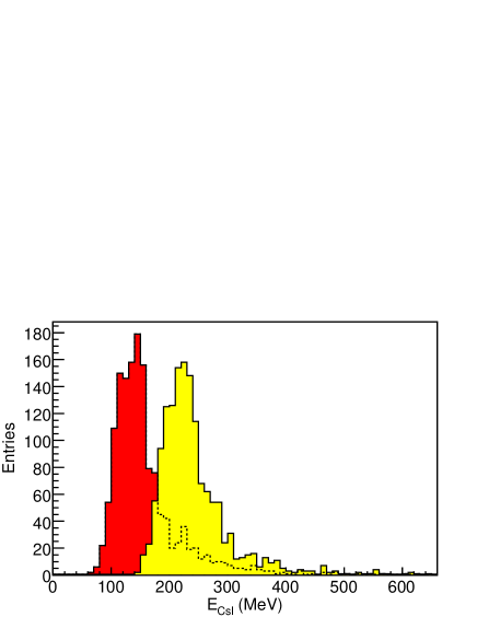
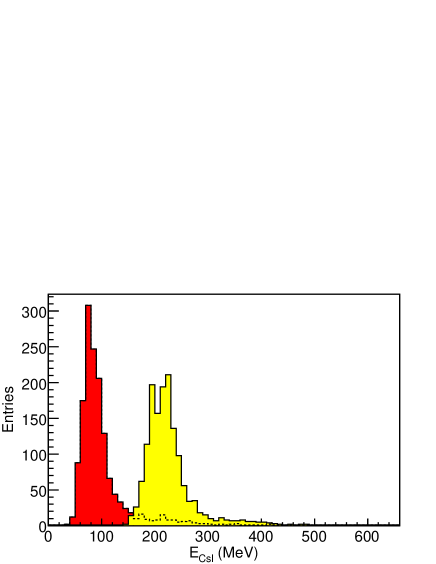
Figure 59: Two examples of energy distributions for events in the central CsI crystal, taken with spectrometer current $I_{\rm S}=160$ A; (left) positrons, (right) electrons. Within each plot the left histogram is for undulator off (out of time) and the right histogram is for undulator on.

No correlations of fluctuations in neighboring undulator-on and -off events were observed. Hence, there was no advantage to a background subtraction based only on neighboring events. Rather, the energy deposition $E_{j}^{\rm off}$ in every undulator-off event of a cycle was subtracted from energy $E_{i}^{\rm on}$ of every undulator-on event of that cycle. The signal $I$ in the beam toroid BT was used to correct for variation in the intensity of the primary electron beam from event to event. This resulted in $n_{\rm on}n_{\rm off}$ background-subtracted energies of the form

$$E_{i}^{\rm on}-E_{j}^{\rm off}\frac{I_{i}^{\rm on}}{I_{j}^{\rm off}}\,,$$ (23)

from a cycle of $n_{\rm on}$ undulator-on events and $n_{\rm off}\approx n_{\rm on}$ undulator-off events.

Signals in the silicon detector P1 (Sec. 3.5.4), just upstream of reconversion target T2, showed a small asymmetry, $\delta^{\sf P1}$, with respect to the polarity of magnet TP1 (see Table 21). This was probably caused by the fringe field of magnet TP2 in conjunction with the misalignment of the positron beam (Sec. 4.3.4). The asymmetries $\delta^{\sf P1}$ varied from $-3$ to $-16$ % of the asymmetries $\delta$ measured in the central CsI crystal for positrons, and was $+40$ % of the asymmetry for electrons. Correction for this effect was made by renormalizing the subtracted energy depositions (23) in the CsI crystal to the (subtracted and normalized by the beam toroid) signal in detector P1, defining renormalized, background-subtracted energies $S_{ij}$ according to

$$S_{ij}=\frac{E_{i}^{\rm on}-E_{j}^{\rm off}\frac{I_{i}^{\rm on}}{I_{j}^{\rm off}}}{{\sf P1}_{i}^{\rm on}-{\sf P1}_{j}^{\rm off}\frac{I_{i}^{\rm on}}{I_{j}^{\rm off}}}\,.$$ (24)

An example of a distribution of renormalized, background-subtracted energies is shown in Fig. 60.

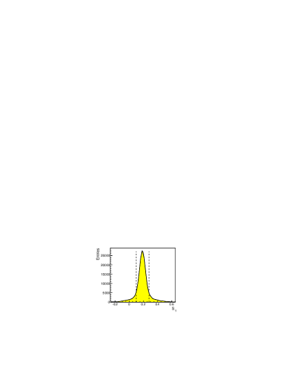
Figure 60: The distribution of renormalized, background-subtracted energies $S_{ij}$, defined in Eq. (24), in the central CsI crystal for a typical data cycle. The dotted lines indicate the $\pm 2\,\sigma$ fit range described in the text.

The multiple use of each event was accounted for in the computation of statistical uncertainties (Sec. 7.4).

The distributions of the $S_{ij}$ had a roughly Gaussian core and relatively long tails to both sides. These tails were excluded by an iterative procedure in which each distribution of the $S_{ij}$ was fit to the sum of two Gaussian functions with common mean but different variances; entries were then cut outside a $\pm 2\,\sigma$ range defined by the narrower Gaussian, after which the mean of the remaining entries was determined by a new fit to two Gaussians.

Alternatively, the truncated mean over a cycle of the renormalized energy $S$ (per positron) in a CsI crystal could be defined as

$$\left\langle S\right\rangle=\left\langle S_{\rm on}-S_{\rm off}\right\rangle=\frac{1}{n_{\rm on}n_{\rm off}}\sum_{i=1}^{n_{\rm on}}\sum_{j=1}^{n_{\rm off}}S_{ij},$$ (25)

where the sum is over only those $S_{ij}$ that pass the cut on the tails of their distribution.

If instead the entries in a distribution of background-subtracted events were the result of subtraction of undulator-off events only from the preceding undulator-on event, a cut on the tails of the distribution would exclude both the undulator-on and the undulator-off event if either one of them had a large fluctuation. The advantage of a procedure based on Eqs. (24)–(25) compared to use of a neighboring event subtraction was the ability to cut on large fluctuations in energies while retaining good statistical power from events with behavior near the mean. Note that without cuts on fluctuations, the mean $\left\langle S_{\rm on}-S_{\rm off}\right\rangle$ in (25) would be equal to $\left\langle S_{\rm on}\right\rangle-\left\langle S_{\rm off}\right\rangle$, and then would not be dependent on any signal-background ordering.

The effectiveness of this method and, in particular, the assignment of uncertainties to the asymmetries derived therefrom, has been verified by Monte Carlo simulations. The mean of a truncated distribution as given by Eq. (25) was found to be a more stable measure of the average signal of a cycle.

The statistical uncertainties on the means $\left\langle S\right\rangle$ of Eq. (25) were calculated from the full width at half maximum of the distribution of the $S_{ij}$ and the numbers of signal events, $n^{\prime}_{\rm on}$, and of background events, $n^{\prime}_{\rm off}$, that contributed to the truncated mean:

$$\Delta\left\langle S\right\rangle=\frac{\sigma_{\left\langle S\right\rangle}}{\sqrt{2}}\cdot\sqrt{\frac{1}{n^{\prime}_{\rm on}}+\frac{1}{n^{\prime}_{\rm off}}}\approx\frac{\sigma_{\left\langle S\right\rangle}}{\sqrt{n^{\prime}}}\,,$$ (26)

where $n^{\prime}=n^{\prime}_{\rm on}\approx n^{\prime}_{\rm off}$ and $\sigma_{\left\langle S\right\rangle}={\rm FWHM}/2.35$ is the width parameter of the approximately Gaussian central distribution of the $S_{ij}$. Taking $\eta$ to be the fraction of entries in the distribution (24) that survived the cuts (see Fig. 60), the quantities $n^{\prime}_{\rm on}$ and $n^{\prime}_{\rm off}$ were defined as:

$$n^{\prime}_{\rm on}=\eta\cdot n_{\rm on}\,,\qquad n^{\prime}_{\rm off}=\eta\cdot n_{\rm off}\,,$$ (27)

where $n_{\rm on}$ and $n_{\rm off}$ are the numbers of signal and background events of a cycle. For the central CsI crystal, $\eta$ was between 77 and $80\,\%$ (see Table 20).

The systematic uncertainties were small, as confirmed by repeating the background subtraction with different methods and independent analyses. For example, an analysis was performed by first averaging (for each crystal) all signal and all background data independently, before the background was subtracted. The results obtained with this alternative procedure were fully consistent with the results presented here.

7.4 Asymmetry Determination

The asymmetries

$$\delta_{k}=\frac{S_{k}^{-}-S_{k}^{+}}{S_{k}^{-}+S_{k}^{+}}\;,$$ (28)

were obtained from the renormalized, background-subtracted energy depositions $S^{-}_{k}$ and $S^{+}_{k}$ of Eq. (25) in the CsI calorimeter for $-$ and $+$ polarity of magnet TP1 during cycle pair $k$, and the corresponding uncertainties $\Delta\delta_{k}$ evaluated as

$$\Delta\delta_{k}=\frac{2\sqrt{\left(S_{k}^{+}\;\Delta S_{k}^{-}\right)^{2}+\left(S_{k}^{-}\;\Delta S_{k}^{+}\right)^{2}}}{\left(S_{k}^{-}+S_{k}^{+}\right)^{2}}\;,$$ (29)

where $\Delta S_{k}^{-}$ and $\Delta S_{k}^{+}$ were determined according to (26). As an example, the asymmetries obtained for all cycle pairs of one spectrometer setting are shown in Fig. 61.

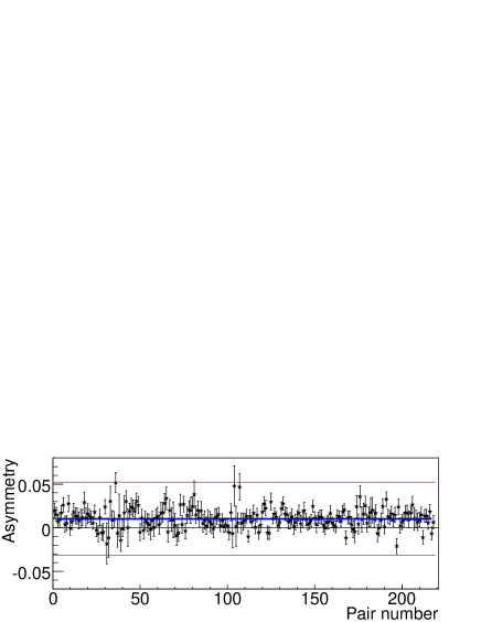
Figure 61: The asymmetries $\delta_{k}$ observed for the 218 cycles pairs in the positron polarimeter for $I_{\rm S}=140$ A during the second running period. Also shown is the best-fit $\delta=\left\langle\delta_{k}\right\rangle$ (horizontal blue line) and the $\pm 3\sigma$ band used for the cut on outliers.

The best-fit value $\delta$ for the asymmetry for each positron energy (setting of spectrometer D2) was determined by fitting a constant to the $\delta_{k}$, taking their uncertainties into account. To exclude possible outliers, only asymmetries within a $\pm 3\sigma$ range were used in the fit. The effect of outliers was small, and was included in the estimate of the systematic uncertainties (Sec. 7.5).

The best-fit asymmetries $\delta$ with uncertainties $\Delta\delta$, and the $\chi^{2}$ per degree of freedom of the fits are listed in Table 21. The uncertainty $\Delta\delta$ is smaller than the standard deviation $\sigma$ of the asymmetries $\delta_{k}$ prior to the exclusion of outliers. Also listed are the asymmetries $\delta^{\sf P1}$ observed in the detector P1, just upstream of magnet TP1. A separate study showed that if the normalization to detector P1 were not done as in Eq. (24), then the asymmetries $\delta$ would have been roughly the sum of the asymmetries $\delta$ and $\delta^{\sf P1}$ given in Table 21.

Table 21: Best-fit asymmetries $\delta$ of Eq. (28) (with respect to the polarity of magnet TP1) measured in the central CsI crystal for all settings of spectrometer D2, together with the $\chi^{2}$ per degree of freedom of the fits. Also listed are the asymmetries $\delta^{\sf P1}$ observed in detector P1.

IS	Etot(e±)	$\delta\pm\Delta\delta$	$\chi^{2}/n_{\rm df}$	$\delta^{\sf P1}\pm\Delta\delta^{\sf P1}$
(A)	(MeV)	(%)		(%)
100	4.59	0.689 $\pm$ 0.165	166.4 / 203	$-$0.115 $\pm$ 0.017
120	5.36	0.961 $\pm$ 0.083	167.9 / 184	$-$0.066 $\pm$ 0.020
140(1)	6.07	1.197 $\pm$ 0.145	404.1 / 276	$-$0.107 $\pm$ 0.110
140(2)	6.07	1.079 $\pm$ 0.063	274.9 / 217	$-$0.055 $\pm$ 0.019
140(1+2)	6.07	1.132 $\pm$ 0.061	628.2 / 490	$-$0.095 $\pm$ 0.034
160(e+)	6.72	0.923 $\pm$ 0.080	257.9 / 166	$-$0.035 $\pm$ 0.023
160(e-)	6.72	0.938 $\pm$ 0.051	167.2 / 144	$+$0.382 $\pm$ 0.022
180	7.35	0.886 $\pm$ 0.196	59.8 / 63	$-$0.108 $\pm$ 0.063
180(ff)	7.35	0.995 $\pm$ 0.140	174.2 / 101	$-$0.081 $\pm$ 0.055

7.5 Systematic Uncertainties

Table 22: Estimates of maximum systematic uncertainties of the asymmetries $\delta$ (Table 21) from various sources.

	Source	Relative
		uncertainty
a)	Non-stat. fluctuations per cycle pair	7 %
b)	Outlier rejection ($\pm 3\sigma$)	8 %
c)	Beam-current cut	5 %
d)	Cycle pairing	9 %
e)	Background correction	7 %
f)	Stray-field-induced asymmetry in P1	5  % $(e^{+})$
		12 % $(e^{-})$

The calculation of the asymmetries $\delta$ assumed that the measurements of energies $E^{+}$ and $E^{-}$ in the central CsI crystal for polarities + and $-$ of magnet TP1 were performed under identical conditions. Differences in those conditions could lead to systematic uncertainties in the asymmetries, whether or not corrections were made for the differences. The various sources of systematic uncertainty on the measurements of the electron/positron asymmetries $\delta$ that were considered are listed in Table 22. Estimates of the systematic uncertainties were made separately for each data set reported in Table 21, and the maximum uncertainty for any data set is listed in Table 22. These uncertainties were later combined with those on the analyzing power $A_{e^{\pm}}$ and on the polarization $P^{\rm Fe}_{e^{-}}$ of the iron in magnet TP1 to evaluate the systematic uncertainties in the polarization $P_{e^{\pm}}$ (Sec. 7.7).

• A measure of non-Gaussian fluctuations in the data is that the $\chi^{2}$ per degree of freedom for the fits to the asymmetries $\delta$ was larger than 1 in some cases. Since for each energy point the individual asymmetries $\delta_{i}$ were statistically independent, a $\chi^{2}$ test can be performed on the statistical nature of the fluctuations. To obtain $\chi^{2}/{\rm ndf}\leq 1$ in all cases the uncertainties on the $\delta_{i}$ must be scaled up by as much as 7%, which was taken as the maximum systematic uncertainty due to non-Gaussian statistics.

• The best-fit asymmetries $\delta$ were also calculated without making the cut on “outliers”, as described in Sec. 7.4. The resulting changes in the $\delta$s were up to 8%, which was taken as the systematic uncertainties associated with the “outlier” cut.

• The influence of the quality cuts on the beam current ($\pm 3\sigma$, Sec. 7.2) and on the background-subtracted energy distributions ($\pm 2\sigma$, Sec. 7.3) was investigated. Variation of these cuts between zero and their nominal values led to changes in the determined asymmetry of up to 5 %, which was taken as the systematic uncertainties associated with these cuts.

• The combination of cycles into pairs is arbitrary, in principle, although our practice of combining adjacent cycles with “+” and “$-$” magnet polarity may have reduced effects of long-term changes. Studies in which cycles were paired at random showed relative changes in the asymmetries of up to 9 %, which was taken as the systematic uncertainties associated with cycle pairing.

• To study whether the backgrounds in signal (undulator-on) and background (undulator-off) events were the same, target-out data (Sec. 5.2) were used to compare the undulator-on and -off energies in the central CsI crystal. The contribution to the systematic uncertainty in the asymmetry from this was thereby estimated to be at most 7%.

• The relative systematic uncertainty due to the renormalization (24) of the CsI-crystal energies to the signal in detector P1 was taken to be 0.3 of the ratio of the P1 asymmetry to the asymmetry $\delta$.

Two other systematic effects entered in the determination of the final positron polarization: the uncertainty of the electron polarization in the core of the analyzer magnet of about 3 % (Sec. 3.5.5), and the systematic uncertainty of 7 % in the simulation of the analyzing power (Sec. 4.4.1).

7.6 Asymmetry Results

The results of the asymmetry analysis are summarized in Table 23. Only the asymmetries for the central CsI crystal (Fig. 62) are reported here, as these are the most significant with respect to the combination of statistical and systematic errors. However, within these uncertainties the measured asymmetries are consistent with expectations from simulation for all crystals (Sec. 4.4.2).

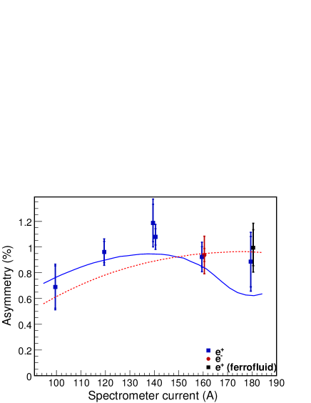
Figure 62: The asymmetries $\delta$ and their total uncertainties (statistical and systematic combined in quadrature) measured at different spectrometer settings with the central crystal of the CsI calorimeter. The solid curve (positrons) and dashed curve (electrons) are from simulations described in Sec. 4.4.2.

7.7 Positron Polarization

The longitudinal polarization of the positrons (electrons) was determined from the relation

$$P_{e^{\pm}}=\frac{\delta}{A_{e^{\pm}}P_{e^{-}}^{\rm Fe}}\,,$$ (30)

where the analyzing power $A_{e^{\pm}}(E)$ was determined for different positron energies $E$ by simulation (Sec. 4) and the effective polarization of the electrons in the iron of magnet TP1 was $P_{e^{-}}^{\rm Fe}=0.0695\,\pm\,0.0021$ (Table 7 and Sec. 7.5). The results are listed in Table 23.

Table 23: Asymmetry ($\delta$), analyzing power ($A$), and polarization ($P$) determined from the central CsI crystal at different spectrometer settings. The systematic uncertainties are the combinations of all systematic effects described in Sec. 7.5.

$I_{\rm S}$	$E_{\rm tot}$	$\delta\pm\Delta\delta_{\rm stat}\pm\Delta\delta_{\rm syst}$					$A\pm\Delta A_{\rm stat}$	$P\pm\Delta P_{\rm stat}\pm\Delta P_{\rm syst}$
(A)	(MeV)			(%)			(%)			(%)
100	4.59	0.69	$\pm$	0.17	$\pm$	0.06	0.1498 $\pm$ 0.0016	66.22	$\pm$	15.90	$\pm$	7.87
120	5.36	0.96	$\pm$	0.08	$\pm$	0.06	0.1563 $\pm$ 0.0015	88.50	$\pm$	7.70	$\pm$	8.62
140(1)	6.07	1.20	$\pm$	0.15	$\pm$	0.12	0.1616 $\pm$ 0.0014	106.56	$\pm$	12.98	$\pm$	13.14
140(2)	6.07	1.08	$\pm$	0.06	$\pm$	0.07	0.1616 $\pm$ 0.0014	96.10	$\pm$	5.69	$\pm$	9.80
140(1+2)	6.07	1.13	$\pm$	0.06	$\pm$	0.08	0.1616 $\pm$ 0.0014	100.75	$\pm$	5.54	$\pm$	10.23
160(e+)	6.72	0.92	$\pm$	0.08	$\pm$	0.08	0.1651 $\pm$ 0.0013	80.47	$\pm$	7.02	$\pm$	9.40
160(e-)	6.72	0.94	$\pm$	0.05	$\pm$	0.14	0.1528 $\pm$ 0.0014	88.29	$\pm$	4.86	$\pm$	14.55
180	7.35	0.89	$\pm$	0.20	$\pm$	0.12	0.1686 $\pm$ 0.0013	75.58	$\pm$	16.72	$\pm$	11.60
180(ff)	7.35	1.00	$\pm$	0.14	$\pm$	0.13	0.1686 $\pm$ 0.0013	84.91	$\pm$	11.99	$\pm$	12.69

Both the statistical and systematical uncertainties in the measured polarizations were determined by the usual error propagation from the uncertainties of the quantities entering (30), $\delta$, $A_{e^{+}}$, and $P_{e^{-}}^{\rm Fe}$.

Comparison in Fig. 63 of the measured polarization as a function of energy with simulation (Sec. 4.4.2) demonstrates good agreement with expectations. Figure 63 does not include the result of the first run at $I_{\rm S}=140$  A during which the beam conditions were somewhat unstable and the resulting uncertainty large, nor the run with ferrofluid in the undulator, which altered the distributions of photon and positron energy and polarization somewhat.

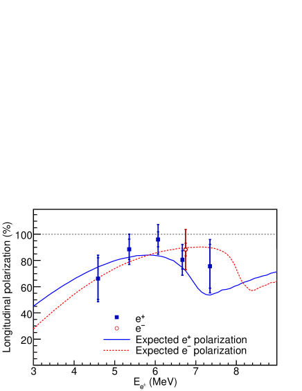
Figure 63: Longitudinal polarization for positrons and electrons as deduced from the asymmetries (28) in the central CsI crystal only. The measurements are compared to the predictions from simulations.

The one measurement of electron polarization also agrees with expectations and thus confirms that systematic effects, which could be different for electrons and positrons, were under control in the analysis.

8 Summary

Experiment E166 has successfully demonstrated a method for producing polarized positrons suitable for the next generation of linear colliders. The method uses a high-energy electron beam in conjunction with a short-period, helical undulator to produce circularly polarized photons with energies of several MeV. The photons are converted in a thin target to generate longitudinally polarized positrons. The tools, techniques, and methodologies developed for the experiment are directly applicable to the design of polarized positron sources for the ILC and for CLIC.

The experiment was carried out with a one-meter-long, 400-period, pulsed helical undulator installed in the Final Focus Test Beam (FFTB) at SLAC. A low-emittance, 10 Hz, 46.6 GeV electron beam passing through this undulator generated circularly polarized photons in the MeV range, with a cutoff energy of the first harmonic at about 7.9 MeV.

These polarized photons were then converted to polarized positrons (and electrons) via pair production in a thin tungsten target. The experiment measured the flux and polarization of the undulator photons, and the spectrum and polarization of the positrons generated in the production target. The photon polarization was determined by measuring the transmission asymmetry in polarized iron. To determine the positron polarization the same method was applied to photons generated by the positrons in a “reconversion target”.

After installation and commissioning of the experiment in the FFTB beam line in 2004, data were collected in two run periods of about 4 weeks each in June and September 2005.

For a detailed comparison of the results with predictions, the Geant4 simulation package has been extended to include all relevant polarization effects of electrons, positrons, and photons in matter. Thus, experiment E166 directly tested the validity of the software used to simulate the physics of polarized pair production in matter and the subsequent polarization-dependent electromagnetic interaction processes in finite thicknesses of matter. This resulting improvement in the simulations leads to greater confidence in the proposed designs of polarized positron sources for the next generation of linear colliders.

Positron polarization was measured at five energy settings of the analyzing spectrometer. In addition, an electron polarization measurement was done at a single energy setting by reversing the polarity of the spectrometer. Over the measured energy range of 4–8 MeV, the positron (and electron) polarization was about 80 % with a relative measurement error of about 10 % to 15 %, dominated by the systematic uncertainties. The measured polarization values agree well with expectations from detailed simulations.

The E166 experiment sucessfully demonstrated the technique of undulator-based production of polarized positrons. The observed performance of undulator, collection, and analyzing systems as well as the photon and positron polarization measurements serve to validate the underlying design methodologies. The modeling tools developed for E166 are now being used to design polarized positron sources for the next generation of linear colliders.

References

- [1]
-
[2]
International Linear Collider Reference Design Report
(Aug. 2007), http://www.linearcollider.org/rdr - [3] R.W. Assmann et al., A 3 TeV Linear Collider based on CLIC Technology, CERN 2000-008 (28 July 2000).
- [4] G. A. Moortgat-Pick et al., The role of polarized positrons and electrons in revealing fundamental interactions at the Linear Collider, arXiv:hep-ph/0507011; Phys. Rep. 460 (2008) 131.
- [5] H. Olsen and L. C. Maximon, Photon and Electron Polarization in High-Energy Bremsstrahlung and Pair Production with Screening, Phys. Rev. 114 (1959) 887.
- [6] P.W. Zitzewitz et al., Spin Polarization of Low-Energy Positron Beams, Phys. Rev. Lett. 43 (1979) 1281.
- [7] V. E. Balakin and A. A. Mikhailichenko, The Conversion System for Obtaining High Polarized Electrons and Positrons, Budker Institute of Nuclear Physics, BINP 79-85 (1979).
- [8] R. C. Wingerson, “Corkscrew” – A Device for Changing the Magnetic Moment of Charged Particles in a Magnetic Field, Phys. Rev. Lett. 6 (1961) 446.
- [9] D. F. Alferov, Yu. A. Bashmakov and E. G. Bessonov, Generation of Circularly Polarized Electromagnetic Radiation, Sov. J. Tech. Phys. 21 (1976) 1408 .
-
[10]
E. G. Bessonov,
Some Aspects of the Theory and Technology of the Conversion Systems of Linear Colliders,
Proc. 15th Intl. Conf. on High Energy Accel. (Hamburg, 1992), p. 138;
E. G. Bessonov and A. A. Mikhailichenko, Some Aspects of Undulator Radiation Forming for Conversion System of the Linear Collider, Budker Institute of Nuclear Physics, BINP 92-43 (1992). - [11] T. Omori et al., Efficient Propagation of Polarization from Laser Photons to Positrons through Compton Scattering and Electron-Positron Pair Creation, Phys. Rev. Lett. 96 (2006) 114801.
- [12] T. Hirose, Proc. Intl. Workshop on Physics and Experiments with Linear Colliders (Morioka, Iwate, Japan, September 8-12, 1995, World Science, Singapore, 1996), pp. 748-756.
- [13] T. Okugi et al., Proposed Method to Produce a Highly Polarized Beam for Future Linear Colliders, Jpn. J. Apl. Phys. 35 (1996) 3677.
- [14] G. Alexander et al., Undulator-based production of polarized positrons: A proposal for the 50-GeV beam in the FFTB, SLAC-TN-04-018 (June 2003).
- [15] G. Alexander et al., Observation of Polarized Positrons from an Undulator-Based Source, Phys. Rev. Lett. 100 (2008) 210801.
- [16] V. Balakin et al., Focusing of submicron beams for TeV Scale linear colliders, Phys. Rev. Lett. 74 (1995) 2479;M. Berndt et al., Final focus test beam: Project design report, SLAC-R-376 (Mar. 1991).
- [17] R. Erickson et al., SLAC Linear Collider Design Handbook, SLAC-R-714 (Dec. 1984).
- [18] A. Mikhailichenko, Pulsed Micro-Undulator for Polarized Positron Production, CBN 05-2 (Cornell, LEPP, Jan. 29, 2005).
- [19] A. Mikhailichenko, Usage of Ferrofluid for Improvement Parameters of Micro-Magnet, CBN 04-3 (Cornell, LEPP, Apr. 12, 2004).
- [20] MERMAID – MEsh oriented Routine for MAgnet Interactive Design, SIM Limited, Novosibirsk, P.O. Box 402, Russia.
- [21] H. Schopper, Measurement of Circular Polarization of -rays, Nucl. Instr. and Meth. 3 (1958) 158.
- [22] S. Agostinelli et al. (Geant4 Collaboration), Geant4: A simulation toolkit, Nucl. Instr. and Meth. A 506 (2003) 250.
- [23] J. Allison et al. (Geant4 Collaboration), Geant4 developments and applications, IEEE Trans. Nucl. Sci. 53 (2006) 270.
- [24] R. Dollan, K. Laihem and A. Schälicke, Monte Carlo based studies of a polarized positron source for International Linear Collider (ILC), Nucl. Instr. and Meth. A 559 (2006) 185; A. Schälicke, K. Laihem and P. Starovoitov, Polarised Geant4– Applications at the ILC, DESY 07-202 (Nov. 2007).
-
[25]
A. Schälicke, K. Laihem, and P. Starovoitov, in preparation; see also chap. Polarized Electron/Positron/Gamma Incident, in Geant4 Physics Reference Manual,
http://geant4.cern.ch/support/userdocuments.shtml - [26] B. M. Kincaid, A Short-period Helical Wiggler as an Important Source of Synchrotron Radiation, J. Appl. Phys. 48 (1977) 2684.
- [27] J. P. Blewett and R. Chasman, Orbits and Fields in the Helical Wiggler, J. Appl. Phys. 48 (1977) 2962.
- [28] A. A. Mikhailichenko, Pulsed Helical Undulator for Test at SLAC. The Polarized Production Scheme, Cornell CBN 02-10, SLAC LCC106 (Sept. 16, 2002).
- [29] J. C. Sheppard, Helical Undulator Radiation, SLAC LCC-0095 (July 2002).
- [30] K. Flöttmann, Investigations Toward the Development of Polarized and Unpolarized High Intensity Positron Sources for Linear Colliders, Ph.D. Thesis, Hamburg University 1993 DESY 93-161.
- [31] L. W. Fagg and S. W. Hanna, Polarization Measurements on Nuclear Gamma Rays, Rev. Mod. Phys. 31 (1959) 711.
- [32] H. Frauenfelder and A. Rossi, Determination of the Polarization of Electrons and Photons, in Methods of Experimental Physics. Nucl. Physics, Part B 5, ed. by L.C.L. Yuan and C.-S. Wu (Academic Press, New York, 1963), pp. 214-274.
- [33] S. B. Gunst and L. A. Page, Compton Scattering of 2.62 MeV Gamma Rays by Polarized Electrons, Phys. Rev. 92 (1953) 970.
- [34] M. Fukuda et al., Polarimetry of Short Pulse Gamma-Rays and Positrons, Proc. 2nd Asian Part. Accel. Conf. (Beijing, China, 2001), p. 881; Polarimetry of short-pulse gamma-rays produced through inverse Compton scattering of circularly polarized laser beams, Phys. Rev. Lett. 91 (2003) 164801.
- [35] J. D. Ullman et al., Determination of Electron and Positron Helicity with Møller and Bhabha Scattering, Phys. Rev. 122 (1961) 536.
- [36] G. G. Scott, Review of Gyromagnetic Ratio Experiments, Rev. Mod. Phys. 34 (1962) 102.
- [37] H.E. Cleaves and J.M. Hiegel, Properties of High-Purity Iron, J. Res. Natl. Bur. Standards 28 (1942) 643.
- [38] R.M. Bozorth, Ferromagnetism (Van Nostrand, New York, 1951), p. 54.
- [39] M.J. Berger et al., XCOM: Photon Cross Sections Database (Nat. Inst. Standards), http://physics.nist.gov/PhysRefData/Xcom/Text/XCOM.html
- [40] K.T. McDonald, Use of a Transmission Polarimeter for a Nonmonochromatic Photon Beam (Oct. 3, 2008), http://puhep1.princeton.edu/~mcdonald/e166/polarimetry.pdf
- [41] F. Corriveau et al., Measurement of the Positron Longitudinal Polarization in Muon Decay, Phys. Rev. D 24 (1981) 2004.
- [42] L. A. Page, Polarization Effects in the Two-Quantum Annihilation of Positrons, Phys. Rev. 106 (1957) 394.
- [43] W.H. McMaster, Matrix Representation of Polarization, Rev. Mod. Phys. 33 (1961) 8.
- [44] R. L. Gluckstern, M. H. Hull, Jr., and G. Breit, Polarization of Bremsstrahlung Radiation, Phys. Rev. 90 (1953) 1026.
- [45] C. Fronsdahl and H. Überall, Polarization of Bremsstrahlung from Polarized Electrons, Phys. Rev. 111 (1958) 580; Nuovo Cim. 8 (1958) 163.
- [46] G. Culligan et al., Longitudinal Polarization of the Positrons from the Decay of Unpolarized Positive Muons, Nature 180 (1957) 751.
- [47] M. Goldhaber, L. Grodzins, and A. W. Sunyar, Evidence for Circular Polarization of Bremsstrahlung Produced by Beta Rays, Phys. Rev. 106 (1957) 826.
- [48] P. C. Macq, K. M. Crowe and R. P. Haddock, Helicity of the Electron and Positron in Muon Decay, Phys. Rev. 112 (1958) 2061.
- [49] S. Bloom et al., Measurement, by Bremsstrahlung Transmission, of the Polarization of from , Phys. Lett. 8 (1964) 87.
- [50] T. Zwart et al., Transmission Polarimetry at MIT Bates: Towards an Absolute Polarimeter?, AIP Conf. Proc. 675 (2003) 1011.
- [51] W.R. Nelson, H. Hirayama and D.W.O. Rogers, The EGS4 Code System, SLAC-Report-265, (1985).
- [52] M. Chodorow and E.L. Chu, Cross-Wound Helices for Traveling-Wave Tubes J. Appl. Phys. 26 (1955) 33.
- [53] A. Mikhailichenko, Conversion system for obtaining polarized electrons and positrons at high energy, CBN 02-13 (Cornell, LEPP, 2002).
- [54] J. Barley, V. Medjidzade and A. Mikhailichenko, New Positron Source for CESR, CBN 01-19 (Cornell, LEPP, 2001).
- [55] Densalloy SD170 is a trademark of Tungsten Products, Madison, AL 35756, USA.
- [56] F. Scholze, H. Rabus, and G. Ulm, Mean energy required to produce an electron-hole pair in silicon for photons of energies between 50 and 1500 eV, J. Appl. Phys. 84 (1998) 2926.
- [57] The D. V. Efremov Scientific Research Institute of Electrophysical Apparatus, Metallostroi 196641, St. Petersburg, Russia, www.niiefa.spb.su
- [58] Model 231P High Power Amplifier, Copley Controls Corp., 20 Dan Road, Canton, MA 02021, USA, www.copleycontrols.com
- [59] OPERA-2d, Vector Fields Inc., 1700 N Farnsworth Ave, Aurora, IL 60505, USA, www.vectorfields.com
- [60] CAN-CAI812 (8 x 12 bit, 10V bipolar ADC) with VME-CAN2 (VMEbus controller), Electronic System Design (ESD) GmbH, Vahrenwalder Str. 207, D-30165 Hannover, Germany, www.esd-electronics.com
- [61] K. Laihem, Measurement of the positron polarization at an helical undulator based positron source for the International Linear Collider ILC, doctoral thesis, Humboldt Universität zu Berlin (2008).
- [62] B. Aubert et al. (BaBar Collaboration), The BaBar detector, Nucl. Instr. and Meth. A 479 (2002) 1.
- [63] J.W. Kovermann, Die polarisierte Positronenquelle E166 – Kalibration des Kalorimeters, Diplomarbeit, RWTH Aachen (Oct. 2006).
- [64] V. Bargmann, L. Michel and V.L. Telegdi, Precession of the Polarization of Particles Moving in a Homogeneous Electromagnetic Field, Phys. Rev. Lett. 2 (1959) 435.
- [65] R. Dollan, Production of polarized positrons and low energy polarimetry at the ILC, doctoral thesis, Humboldt Universität zu Berlin (in preparation).