An iterative filter to reconstruct planetary transit signals in the presence of stellar variability

Abstract

The detrending algorithms which are widely used to reduce the impact of stellar variability on space-based transit surveys are ill-suited for estimating the parameters of confirmed planets, as they unavoidably alter the transit signal. We present a post-detection detrending algorithm, which filters out signal on other timescales than the period of the transit while preserving the transit signal.

We compare the performance of this new filter to a well-established pre-detection detrending algorithm, by applying both to a set of 20 simulated light curves containing planetary transits, stellar variability, and instrumental noise as expected for the CoRoT space mission, and performing analytic fits to the transits. Compared to the pre-detection benchmark, the new post-detection filter systematically yields significantly reduced errors (median reduction in relative error over our sample $\sim 40\%$) on the planet-to-star radius ratio, system scale and impact parameter. This is particularly important for active stars, where errors induced by variability can otherwise dominate the final error budget on the planet parameters.

Aside from improving planet parameter estimates, the new filter preserves all signal at the orbital period of the planet, and thus could also be used to search for light reflected by the planet.

1 Introduction

Accurate measurements of the fundamental parameters of extra-solar planets are needed to constrain theoretical models of planet formation and evolution. For transiting planets, it is possible to measure the radius and true mass, which can be confronted to the predictions of evolutionary models with various compositions and heat deposition mechanisms (e.g. Guillot 2005; Baraffe et al. 2008). These models are continuously challenged by new discoveries, the best known case of this being the small group of planets whose radii are larger than expected for their mass and irradiation level, such as HD 209458b (Charbonneau et al., 2000; Knutson et al., 2007), HAT-P-1b (Bakos et al., 2007; Winn et al., 2007), WASP-1b (Collier Cameron et al., 2007; Charbonneau et al., 2007), TrES-4b (Mandushev et al., 2007), XO-3b (Winn et al., 2008), CoRoT-Exo-2b (Alonso et al., 2008). Giant transiting planets can thus be highly sensitive diagnostics of the validity or otherwise of specific theoretical predictions, but only if their masses and radii can be measured with accuracies of 1–2%. As new detections of smaller transiting planets are expected over the next few years, maintaining this level of accuracy will become more and more challenging. Seager et al. (2007) used simple solid planet structure calculations to show that uncertainties of a few % at most are needed to distinguish between different bulk compositions for sub-Uranus planets using their location in the mass-radius plane – whilst more detailed calculations show that the mass-radius relation of planets with mixed compositions may be degenerate (Adams et al., 2008).

A rapid review of the factors contributing to these uncertainties is helpful at this stage. High precision planetary transit observations allow the direct measurement of the planet-to-star radius ratio $R_{\rm p}/R_{\rm s}$, the system scale (ratio of the semi-major axis to the stellar radius $a/R_{\rm s}$), and the impact parameter $b$ ( $\equiv a/R_{\rm s}\cos i$, where $i$ is the inclination of the orbit).

On the other hand, radial velocity observations of the host star yield a measurement of the planet mass $M_{\rm p}$ relative to the star mass $M_{\rm s}$, convolved with the inclination term $\sin i$ which is known in the case of transits. For a circular orbit:

$$\frac{M_{\rm p}}{M_{\rm s}^{2/3}}=\frac{K}{\sin i}\left(\frac{P}{2\pi G}\right)^{1/3}$$ (1)

where $K$ is the semi-amplitude of the host star’s radial velocity variations, $P$ is the orbital period of the system, $G$ is Newton’s constant of gravitation, and $M_{\rm p}\ll M_{\rm s}$. Combined fits to the transit and radial velocity data can thus be used to measure the relative planet mass and radius ratios.

Obtaining absolute estimates for these parameters requires knowledge of the star mass and radius, which are usually obtained by comparing high-resolution, high signal-to-noise ratio spectra of the star to theoretical models. The transit observations provide a constraint on $M_{\rm s}^{1/3}/R_{\rm s}$, which can be combined with the spectral parameters of the star and theoretical evolutionary tracks to obtain estimates of $M_{\rm s}$ and $R_{\rm s}$.

There are thus three classes of sources of uncertainty on the masses and radii of transiting planets: those arising from the transit fit, those arising from the radial velocity fit, and those arising from the spectral analysis of the host star. The detailed listing of the parameters of published transiting planets and their host stars, maintained at http://www.inscience.ch/transits/ by F. Pont, can be used to perform a basic evaluation of their relative impacts. The combined uncertainties on published transiting planet parameters vary widely, from $\sim 1$% to 11% for $R_{\rm p}$ and to 20% for ${M_{\rm p}}$, depending primarily on the brightness of the host star and the degree to which each system has received detailed characterisation using dedicated follow-up observations. Uncertainties on $M_{\rm s}$ and $R_{\rm s}$, which can reach up to 13% and 17% respectively in some cases, are usually the dominant source of uncertainty for massive (Jupiter-mass and above) planets, which represent the vast majority of the transiting planet crop to date. However, as smaller and lower-mass planets become increasingly detectable thanks to space-based transit searches and improvements in ground-based radial velocity instruments, the uncertainties arising from the transit and radial velocity fits are expected to become more important.

A specific problem arises when the transits become comparable in depth with the amplitude of the intrinsic brightness fluctuations of the host star. These are due to the temporal evolution and rotational modulation of structures on their surface (stellar spots, plages, granulation). The amplitude of these variations can be several orders of magnitude greater than the transit signal, particularly for terrestrial planets and/or active stars, and they can occur on timescales significantly shorter than the orbital period of the planet (see Fig. 1, upper curve). Stellar variability can thus hinder the detection of planetary transits (Aigrain et al., 2004), but a number of ‘pre-detection’ filters have been developed to tackle this problem. The performance of several of these filters in terms of transit detection was evaluated in the context of first CoRoT blind test (Moutou et al. 2005, hereafter M05), a hare-and-hounds exercise involving 1000 simulated CoRoT light curves containing various transit-like signals, stellar variability and instrumental noise. This test showed that the most successful filters recover a detection threshold close to that obtained in the presence of instrumental noise only, except for a few cases involving the most active and rapidly rotating stars simulated.

However, these filters also have the property of modifying the shape of the transit signal (M05, Bonomo & Lanza 2008 hereafter BL08), and would destroy any signal at the period of the transit occuring on longer timescales than a few hours. We therefore set out to develop an alternative algorithm, hereafter referred to as ‘reconstruction filter’, designed to remove variability at other periods than that of the transit but preserve the transit signal, once that period has been determined. We then evaluated the resulting improvement in planet parameter measurements compared to a benchmark pre-detection filter.

After briefly introducing the simulated dataset used for test purposes throughout the paper in Sect. 2, we describe some of the current pre-detection filters in Sect. 3, and quantify the effect of a benchmark filter on the transit signal. We then describe the reconstruction filter and evaluate its effect on the transit signal in the same way in Sect. 4. The impact of the two types of filter on the accuracy of planet parameter measurements are compared in Sect 5, and the main results are summarised in Sect 6.

2 The CoRoT blind test dataset

2.1 The original dataset

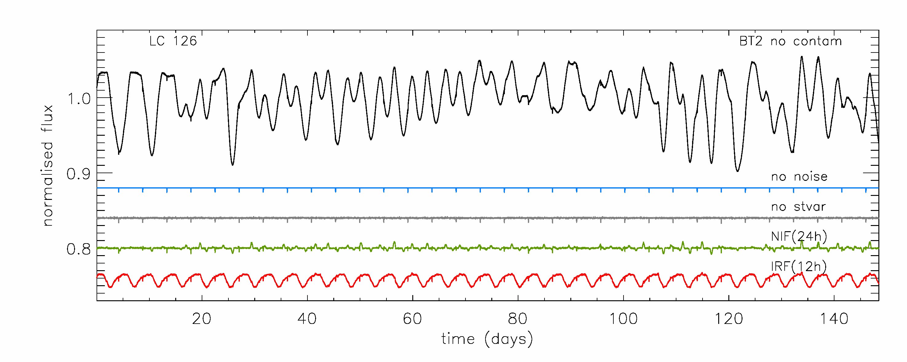
Figure 1: Example of a simulated CoRoT BT2 light curve, corrected from the contaminant flux (2%) coming from a background star (top curve, black line). This light curve contains the transit signal of a Saturn-like planet orbiting a particularly active Sun-like host star with an orbital period of 4.576 d. Below the BT2 light curve are shown, from top to bottom and with a vertical offset for clarity, the no-noise (transits only, blue), no stellar variability (transits plus instrumental noise only, grey) light curves, as well as the NIF-filtered (green) and IRF-filtered (red) versions of the same light curve (see text for details).

The starting dataset used in this study is a sample of 26 simulated CoRoT light curves with planetary transits taken from the second CoRoT blind test (hereafter BT2; Moutou et al. 2007), which was carried out to compare methods for discriminating between planetary transits and grazing or diluted stellar eclipses. The production of the light curves followed roughly the same steps as that for the first CoRoT blind test (BT1), described in detail in M05, incorporating transits simulated with the Universal Transit Modeler (UTM), instrumental noise simulated using the CoRoT instrument model (Auvergne et al., 2003), and stellar variability curve simulated using a combination of the methods of Lanza et al. (2004) and Aigrain et al. (2004).

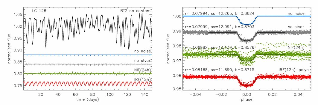
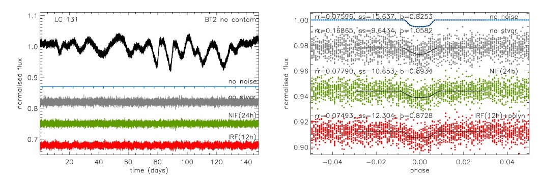
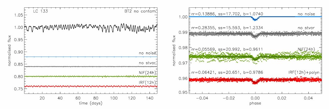
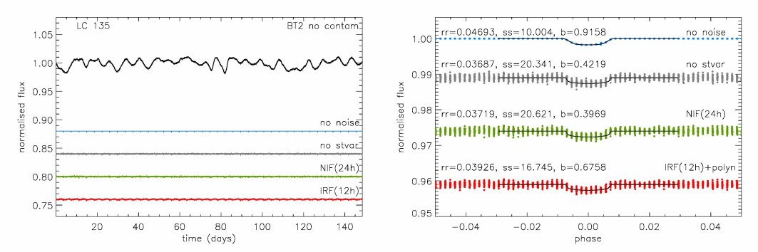
Figure 5: The 20 BT2 light curves in the comparison sample. The light curve number is shown on the plots in the left column (original BT2 numbering scheme) and the planet to star radius ratio (rr), system scale (ss), and impact parameter (b) in the right column.

An updated version of the CoRoT instrument model was used in the BT2, incorporating more realistic satellite jitter and enabling the production of 3-colour light curves, though the 3 bandpasses were summed in the present study to construct a ‘white’ light curve. The two approaches used in the BT1 to model stellar variability were merged in the BT2, using the scaled spot model of Lanza et al. (2004) to simulate rotational modulation of active regions and the stochastic model of Aigrain et al. (2004) to simulate granulation. The simulated transits correspond to planet radii ranging from 0.2 to $1.1\,R_{\rm Jup}$, orbital periods from 2.6 to 11.0 d, and impact parameters from 0.25 to 0.88. As in the BT1, the flux in each aperture was modelled as arising from two stars, only one of which contained a transit-like signal. This is to reflect the fact that there is almost always one or more backgrounds star in the CoRoT aperture. This has the effect of diluting the transit signal, and to account for it we subtracted from each BT2 light curve a constant corresponding to the fraction of the median flux contributed by the star which is not eclipsed (see Tab. 3 in Appendix for contaminant fluxes (percentages of total flux) corrected from in each BT2 light curve studied). An example of a light curve with transit from the BT2 is shown in Fig. 1, and a phase-folded version in Fig. 2. The full set of light curves is shown in Appendix A (Figs. 5 & 10)

2.2 The reference sets

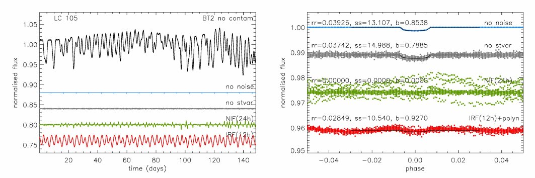
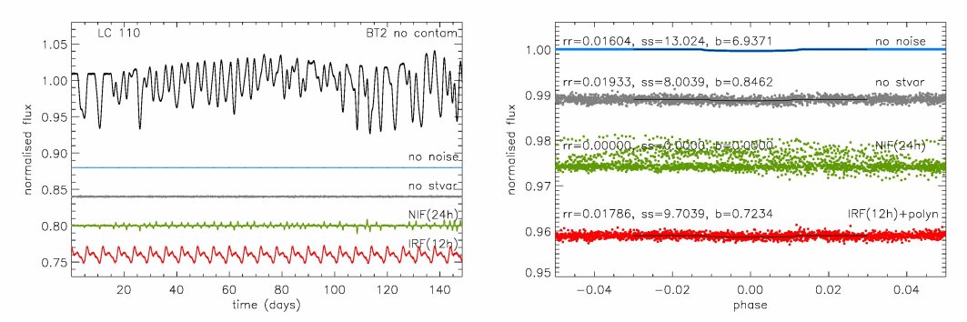
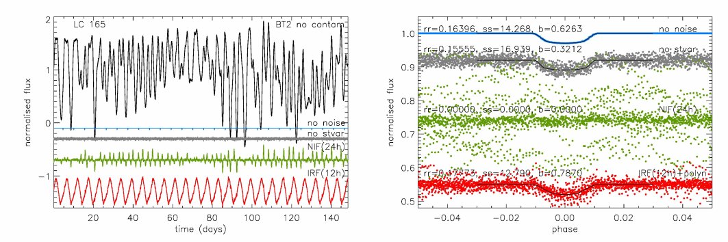
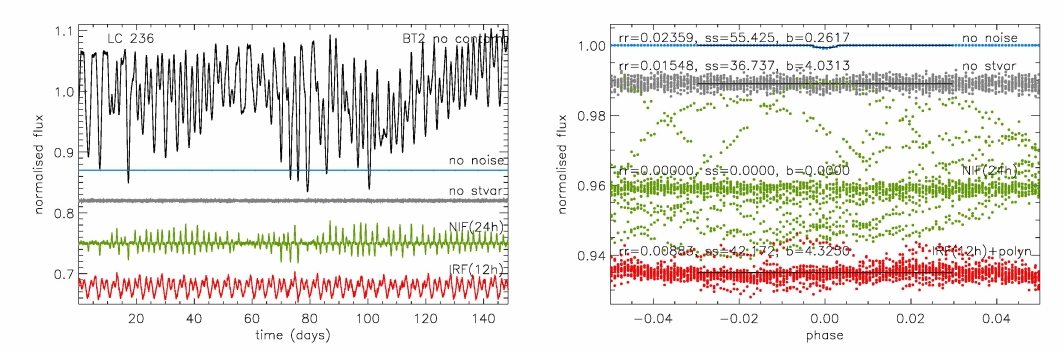
Figure 10: The 4 BT2 transit light curves where the transit was undetectable after applying the NIF and miningful fits to the resulting transits were not possible. Same legend as Fig. 5. These transits became boarder-line detectable in the IRF-filtered light curves.

As we are using simulated data, each component of the signal is known and can be studied individually. We have thus constructed two sets of reference light curves, using on one hand only the transit signal (no noise, no stellar variability) and on the other hand the transit signal and instrumental noise only (no variability). We use the first set to evaluate the reference values of the parameters derived from transit fits in Sects. 3 to 5. These could have simply been deduced from the input parameters given to the transit modelling software UTM when simulating the light curve. However, there can be differences between those and the parameters recovered from the transit fit due to the fitting process, rather than to the noise, and we wish to keep those effects, which are not specifically of interest here, separate from the effects of the stellar and instrumental noise. The second set was used to provide a benchmark for how well one can measure the parameters of interest in the presence of instrumental (white) noise, i.e. if the stellar variability was removed perfectly. These reference sets are shown in blue and grey respectively in Figs. 1, 2, 5 and 10.

After visual analysis of our two reference sets of light curves, we discarded two of the 26 light curves, where the transits were so small as to be undetectable even in the light curves with no stellar variability, as such cases would not realistically reach the post-detection stage.

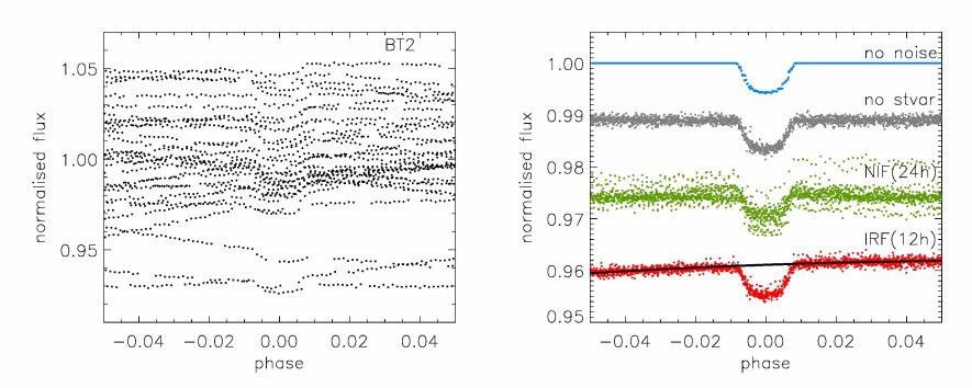
Figure 2: Phase-folded plots of the light curves shown in Fig. 1. Left: original BT2 light curve. Right: from top to bottom, no noise (blue), no variability (grey), NIF-filtered (green) and IRF-filtered (red). The black line overplotted on the IRF-filtered light curve is a $2^{nd}$ degree polynomial fit about the transit, by which the filtered light curve is divided before fitting the transit.

3 Effect of pre-detection filters

3.1 The benchmark pre-detection filter

Pre-detection filters aim to remove stellar variability in light curves to improve the detectability of transits, without any prior knowledge of the transit signal except for the fact that stellar variability typically occurs on longer time scales (hours to days) than the transit signal (minutes to hours). All of the techniques tested in the CoRoT BT1, which range from simple Fourier-domain low-pass filters to slightly more sophisticated implementations involving simultaneous fitting of hundreds of low-frequency sinusoids, or time-domain nonlinear iterative filtering (Aigrain & Irwin 2004, hereafter AI04), exploit this difference. These filters proved effective in removing stellar variability to facilitate the detection of transits but, as pointed out in M05 and BL08, they deform the shape of the transits. In this section, we quantify the impact of the deformation cause by the nonlinear iterative filter (NIF) of AI04 on the derived planet parameters. The NIF performance as a pre-detection filter was recently compared to a range of other published methods (BL08), and it emerged as the method of choice among those compared. The NIF is used by the new filter described in this paper, to estimate the light curve continuum. These two reasons make the NIF a suitable benchmark for the present work, providing us with a direct evaluation of improvement in filtering performance.

The NIF separates stellar variability from the transit signal in the time domain, using an iterative procedure with the following steps:

1. apply a short base-line (here we use 7 data-points, $\sim$1 hour) moving median filter to smooth out the white noise and reduce the sharpness of any high-frequency features in the data;

2. apply a longer base-line (here we use 24 hours) moving median filter to the output of the step (i), followed by a shorter base-line (here we use 2 data-points, $\sim$17 minutes) boxcar (moving average) filter;

3. subtract the output of step (ii) from that of step (i) and evaluate the scatter of the residuals as $\sigma=1.48\times{\rm MAD}$, where ${\rm MAD}$ is the median of the absolute values of the residuals;

4. flag all outliers differing by more than $n\sigma$ from the continuum;

5. return to step (ii) and repeat the process, interpolating over any flagged data points before estimating the continuum and excluding them when estimating the scatter of the residuals, until convergence is reached (typically less than 3 iterations);

6. subtract the final continuum from the original light curve.

As the procedure converges, more and more of the in-transit points become flagged at step (iv), so that the effect of the transits on the final continuum estimate is minimal. However, the choice of long base-line for the moving median filter in step (ii) and of $n$ in step $(iv)$ must reflect a trade-off between appropriately following the stellar variations and incorporating too much of the transit signal when evaluating the continuum. This trade-off results in some of the transit signal been unavoidably filtered along with the variability. For the value of $n$ in step $(iv)$, one would normally use $n=3$ to flag more in-transit points. In the case of the BT2, some light curves contain very strong and rapid variability. Thus, using a low $n$ would clip not only in-transit points but also out-of-transit points where the variability is too rapid to be well modelled by the continuum estimate (as in the example in Fig. 1). Hence, we used $n=150$ in this paper, which effectively means no points are clipped and convergence occurs at the first iteration.

3.2 Quantitative impact on transit parameters

We applied the NIF (Section 3.1) to our sample of 24 BT2 light curves. The post-NIF light curves are shown in green on Figs. 1, 2, 5 and 10. Clear variability residuals are visible in the unfolded post-NIF curves, corresponding to sections of the light curve where the variability is too rapid to be filtered adequately. The phase-folded light curves also show that the shape of the transits is affected by the filter. In practical terms, the transit appears both shorter and shallower than before filtering.

We then folded all light curves at the period of the injected transits and performed least-squares fits of trapezoidal models to the results to estimate the basic transit parameters: depth $\delta$, internal and external duration $d_{\rm i}$ and $d_{\rm e}$ (respectively excluding and including ingress and egress), and the phase $\phi$. The light curves were normalised such that the out-of-eclipse level is always 1. The same folding and trapeze fitting procedure was applied to the two reference sets described in Section 2.2.

In 4 of the BT2 light curves (Fig. 10), the stellar variability was so strong that, after applying the NIF, the phase-folded transits were barely detectable, and meaningful fits to these transits impossible. These 4 light curves were excluded from the comparison of the NIF filter with noise- and variability-free cases which is discussed below.

We list the measured values of the transit parameters ($\delta$, $d_{\rm i}$ and $d_{\rm e}$) of direct relevance to the determination of planet parameters for all 20 light curves in Appendix B (Table LABEL:tab:trpara). We also show, in Fig. 3, cumulative histograms of the relative error $\sigma(\theta)=|\theta-\theta_{0}|/\theta_{0}$, where $\theta$ is the parameter of interest and the subscript $0$ refers to the value measured from the reference light curve with transits only (no noise), contrasting the NIF case (green dashed line) to the case with no variability (black solid line). The median relative errors obtained with the NIF over our sample are $\sigma_{\rm NIF}(\delta)=12\%$, $\sigma_{\rm NIF}(d_{\rm e})=10\%$ and $\sigma_{\rm NIF}(d_{\rm i})=52\%$, indicating that the planet parameters would be seriously affected if derived from NIF-filtered light curves. We note that the internal duration $d_{\rm i}$ tends to be systematically underestimated even for the reference set of light curves with no stellar variability. For a discussion of the source of this well-known bias, see e.g. Pál (2008).

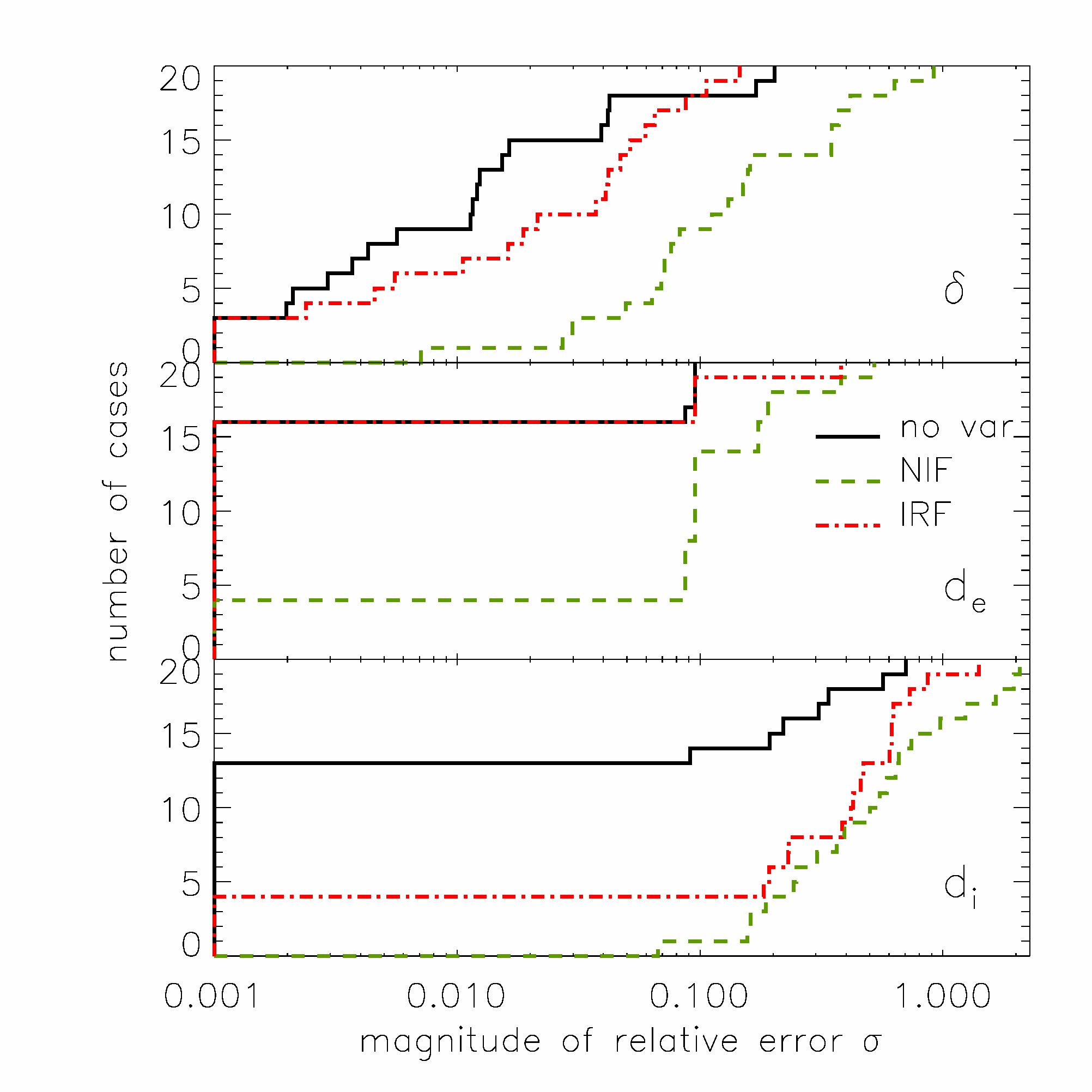
Figure 3: Cumulative histograms of the relative error $\sigma$ (see text for exact definition) on the transit parameters measured from trapezoidal fits to the light curves with no variability (black), NIF-filtered light curves (green) and IRF-filtered light curves (red). Upper panel: transit depth $\delta$; middle panel: external duration $d_{\rm e}$ (total transit duration); lower panel: internal duration $d_{\rm i}$ (duration in full-transit). $\sigma>1$ when a parameter is mis-estimated by more than its true value.

4 A post-detection reconstruction filter

4.1 Definition

In an attempt to avoid the undesirable effects of the NIF on the transit shape, we developed an iterative reconstruction filter (IRF) intended to remove stellar variability once the transits have been detected, whilst altering the transit signal as little as possible.

The IRF is an iterative approximation of the full signal at the period of the transit. It uses the NIF to simultaneously estimate the continuum variation (i.e., stellar variability).

Let $\{Y(i)\}$ (where $i=1$, …, $N$, $N$ being the number of data points in the light curve) represent the observed light curve (which is assumed to be normalised), $\{A(i)\}$ the detrended light curve and $\{F(i)\}$ the signal to be filtered out. We give the main steps of the IRF below:

1. Select an initial estimate for $\{F(i)\}$. We adopt $\{F(i)\}=1$ as our initial estimate.

2. Compute a corrected time-series $\hat{Y}(i)\equiv Y(i)/F(i)$.

3. Estimate $\{\hat{A}(i)\}$ by folding $\{\hat{Y}(i)\}$ at the transit period and boxcar averaging it in intervals of a fixed duration in phase units (binning is used to reduce high frequency noise). For the BT2 light curves, a duration of 0.09% of the phase was found to be suitable (this value was selected by trial and error, longer duration implying lower noise in the estimate of $\{\hat{A}(i)\}$ but more distortion of the transit signal).

4. Unfold $\{\hat{A}(i)\}$ to obtain $\{{A}(i)\}$. Compute a new estimate of $\{F(i)\}$ by applying the NIF to $\{Y(i)/A(i)\}$. The baseline for the median filter used in the NIF at this step can be chosen on a case-by-case basis, and can be significantly shorter than in the pre-detection case, because it is applied to a light curve from which most of the transit signal has been removed. In the present study, we adopt a baseline of 12 hours.

5. Return to step (ii) with the new estimate of $\{F(i)\}$, and iterate until the condition $|\mathcal{D}_{j-1}-\mathcal{D}_{j}|<10^{-4}$ is satisfied for two consecutive iterations, where $j$ is the iteration number (initialisation at $j=0$), and

   $$\mathcal{D}_{j}=\frac{\sum_{i=1}^{N}\left[Y(i)/A_{j}(i)-F_{j}(i)\right]^{2}}{N-1}.$$

   In the case of the BT2 light curves, the convergence was reach after 4 iterations (i.e ${D}_{j}$ was calculated up to $j=6$).

The final detrended light curve is given by $\{Y(i)/F(i)\}$, where $\{F(i)\}$ is the last (presumably best) estimate of the stellar variability.

This algorithm is in some ways analogous to the trend filtering algorithm (TFA) of Kovács et al. (2005) (hereafter KBN05) in post-detection mode. For clarity, we briefly list the main similarities and differences between the two algorithms. The TFA is designed to remove systematic trends common to large numbers of light curves in transit surveys, rather than stellar variability which is individual to each object, but both algorithms work by decomposing each light curve into three components: the signal of interest $\{A(i)\}$ (the transits), the signal to be filtered out $\{F(i)\}$ (the systematics in the case of the TFA and the stellar variability in the case of the IRF), and the residuals. In the TFA, the signal to filter out (systematics) is modeled as a linear combination of a number of template light curves selected from the survey sample. In the IRF, the signal to filter out (stellar variability) is taken as the continuum of the light curve estimated with the NIF (description in Section 3.1). In this analogy, the NIF would be equivalent to TFA in pre-transit-detection mode. When used in reconstruction mode (post-detection), both methods make use of the knowledge of the transit period to iteratively improve the evaluation of the transit signal and of the signal to be filtered out (which is assumed not to be periodic). Whereas $\{F(i)\}$ and $\{A(i)\}$ are treated additively in the TFA, they are treated multiplicatively here since the signal to be filtered out is intrinsic to the star, and the planet hides a certain fraction of the flux emitted by the star. This also results in a different convergence criterion. In KBN05, the first estimate of $\{F(i)\}$ is obtained from the pre-detection implementation of the TFA. In the IRF, it would be counter-productive to use the NIF-filtered light curve as the initial estimate of $\{F(i)\}$, since we have shown that the NIF affects the transit signal we are trying to reconstruct (see Section 3.2), so the inital estimate of $\{F(i)\}$ is taken to be constant at 1. Finally, the IRF treats high frequency effects by smoothing the phase-folded signal, while the TFA treats them by filtering out common outlier values.

4.2 Performance on simulated light curves

The red curves in Figs. 1, 2, 5 and 10, show the light curves in our sample after applying the IRF. Visually, one does not detect any sign of deformation of transit shape. On the other hand, a different feature, which can be seen as a limitation of this filter, is immediately apparent: the IRF preserves any signal at the period of the transit. This property has positive consequences: it implies that potentially interesting signals, such as secondary eclipses, reflected light variations, or thermal emission variations, are preserved. On the other hand, any power in the stellar variability signal at the frequency corresponding to the planet’s orbital period is also preserved. This could be reduced – but not entirely eliminated – by taking the initial estimate of $\{F(i)\}$ to be the continuum estimated with the NIF, but with a base-line long enough not to have a significant impact on the transit signal (though it would remove any slower phase variations associated with the planet). On the other hand, it is straightforward to remove the residual variability about the phase-folded transit, for instance by fitting a low-order polynomial to the data about the transit in the final phase-folded light curve. Dividing the final phase-folded light curve by this polynomial allows to extract a normalised phase-folded transit that can be used to derive the planet parameters. Such a technique is commonly applied to remove variability about each transit in unfiltered, unfolded light curves (see e.g. Alonso et al. 2008). Using it on the folded light curve after applying the IRF significantly reduces the number of free parameters, and thus should increase the reliability of the results. An example of such a fit is shown on Fig. 2.

The IRF was applied to our sample of 24 BT2 light curves, and the residual variability around the transit was removed by subtracting a $2^{nd}$ order polynomial fit of the continuum about the transit. This re-normalisation is important as the trapezoidal fit function used assumes a constant out-of-transit level. The transit parameters were then estimated from a trapezoidal fit to the resulting phase-folded transit in the same way as described in Section 3.2 for the NIF case. The results are listed in Table LABEL:tab:trpara and shown as the red dash-dot curves in Fig. 3. For the 20 BT2 transit light curves which were also used to evaluate the performance of the NIF, the IRF gives median relative errors of $\sigma_{\rm IRF}(\delta)=3\%$, $\sigma_{\rm IRF}(d_{\rm e})<10^{-4}\%$ and $\sigma_{\rm IRF}(d_{\rm i})=$ 42%, representing a significant improvement over the NIF case. Additionally, in the 4 cases where the transits were barely detectable after applying the NIF, which are not included in the comparison sample, the transits are clearly detectable and yield meaningful fits after applying the IRF.

Looking at Fig. 3 in more detail, we see that, where a relative error on the transit depth in excess of 10% (essentially precluding any meaningful constraints on the planet structure) occurs in 60% of the cases studied with the NIF, it occurs in only 5% of the cases with the IRF. Similarly, the NIF yielded $\sigma(\delta)<3\%$ (potentially allowing discrimination between different kinds of evolutionary models as well as a reliable basic structure determination) in only 15% of the cases, but the IRF did so in 50% of the cases.

It is also clear that the external transit duration is recovered near-optimally in the light curves treated with the IRF, with $\sigma(d_{\rm e})<0.1\%$ in 80% of the cases and $\sigma(d_{\rm e})<10\%$ in 95% of the cases, compared to a significantly decreased performance with the NIF. However, although the IRF also systematically improves the determination of the internal transit duration compared to the NIF, this improvement is much less significant, and the relative errors remain large (more than 10% for 80% of the cases studied). This implies that the IRF would probably not significantly increase the number of cases where both internal and external duration can be determined precisely enough to break the degeneracy between system scale and inclination, and thus to constrain the stellar density in a model-independent fashion.

5 Implications for star-planet parameters

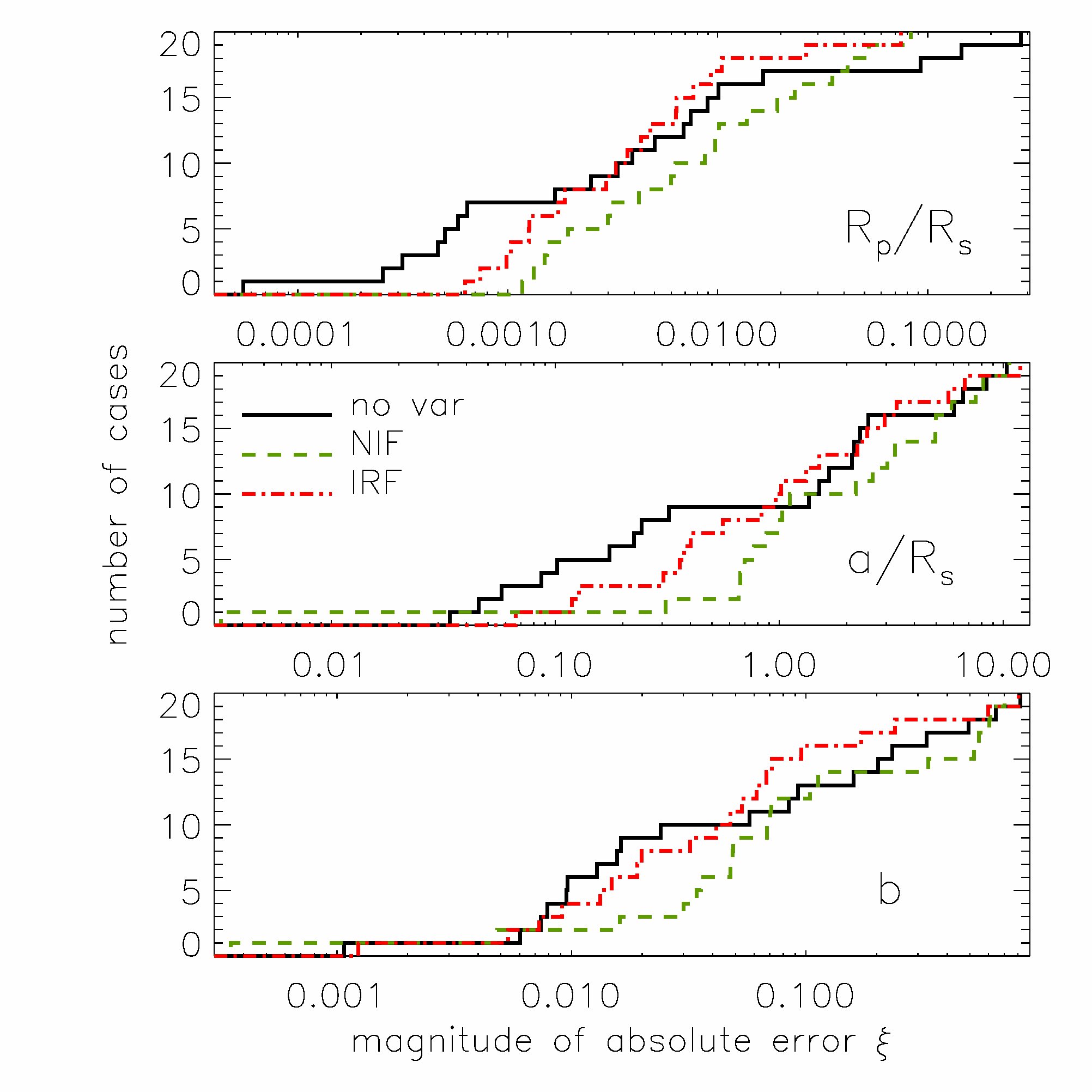
Figure 4: Cumulative histograms of the errors $\xi$ (see text for definition) for star-planet parameters measured from MA02 transit fits to the light curves with no variability (black), NIF-filtered light curves (green) and IRF-filtered light curves (red). Upper panel: radius ratio $R_{\rm p}/R_{\rm s}$; middle panel: system scale $a/R_{\rm s}$; lower panel: impact parameter $b$.

Although the basic trapezoidal fits performed in the previous two sections provide a quick estimate of the degree of deformation of the transit signal due to the variability filtering process, one would in practice perform a full transit fit based on a physical model of the star-planet system. Mandel & Agol (2002) (hereafter MA02) provided an analytical formulation which has become very widely used for such purposes, and was also used to generate the transits injected in the BT2 light curves.

By definition, the IRF preserves any signal at the period of the transit. If the stellar variability contains power at this period, it is preserved, inducing a flux gradient around the transit. This must be removed before fitting, since the MA02 formalism assumes that the out-of-transit level is 1. This was done by fitting a $2^{\rm nd}$ order polynomial fit – the lowest-order found to give satisfactory results – to the data about the transit in the phase-folded curve (based on two segments, each lasting 0.1 in phase, and offset by 0.15 in phase from the center of the transit on either side) before fitting the transits. Note that this is still a significant improvement over the common practice of performing a local polynomial fit to the vicinity of each transit, since the latter option has many more free parameters (one set of free polynomial parameters per transit, rather than one for the entire light curve).

We then used the quadratic limb darkening prescription of MA02 to fit transit models to the 20 BT2 transit light curves where the transits were clearly detectable with both filters. We performed these fits on both reference sets described in Section 2.2 (no noise and no variability), as well as on the BT2 light curves themselves after applying the NIF on the one hand, and the IRF followed by a polynomial fit to the region around the transit on the other hand. The fits were performed using an idl implementation of the Levenberg-Marquart algorithm. The parameters of the model used are the transit epoch $T_{0}$, the period $P$, the system scale $a/R_{\rm s}$ (where $a$ is the semi-major axis), the star-to-planet radius ratio $R_{\rm p}/R_{\rm s}$, the orbital inclination $i$ (or impact parameter $b\equiv a\cos i/R_{\rm s}$), and the quadratic limb-darkening coefficients $u_{a}$ and $u_{b}$. In this study, we fixed the period and limb-darkening coefficients at the values used to build the light curves. The initial epoch was taken directly from the trapezoidal fits. The initial value for $a/R_{\rm s}$ was derived from the period using Kepler’s $3^{\rm rd}$ law, assuming $R_{\rm s}=R_{\odot}$ and $M_{\rm s}=M_{\odot}$. In order to ensure convergence in both grazing and full transits we selected, after some trial and error, an initial inclination of 83.7^∘. We assumed zero eccentricity in all cases (all the transit light curves in our sample were simulated for circular orbits).

The results of the fits are listed in Table LABEL:tab:plpara, while the fits themselves are shown in Figs. 5 and 10. They are also compared in cumulative histogram form in Fig. 4 (with the same colour and line scheme as Fig. 3). Instead of the relative error $\sigma$, we show the absolute error $\xi=|\theta-\theta_{0}|\equiv\sigma\times\theta_{0}$ with respect to the no noise case (subscript 0), for $\theta$ the key planet parameters $R_{\rm p}/R_{\rm s}$, $a/R_{\rm s}$ and $b$.

The IRF provides an overall improvement over the NIF in all three parameters, reducing the median of $\xi(R_{\rm p}/R_{\rm s})$ from 0.007 to 0.003, $\xi(a/R_{\rm s})$ from 1.7 to 1.0, and $\xi(b)$ from 0.07 to 0.04 for $b$. For comparison, the corresponding median values for the the case with no variability are 0.003, 1.4 and 0.07 respectively. However, the situation is not as clear cut as when viewed in terms of transit parameters: there are a few cases where the NIF gives a better match with the parameters obtained from the noise-free light curves, and even cases where the largest error occurs in the light curves containing instrumental noise only.

In an attempt to understand the reason for this, we examined all the light curves one by one (see Figs. 5 and 10). The light curves separate fairly naturally into three broad classes:

1. cases where the IRF performed better than the NIF (transit shape and derived planet parameters closer to the shape and parameter obtained in the absence of stellar variability): light curves 126, 162, 169, 196, 200, and 223. These are cases where the original light curves contain large amplitude, short timescale stellar variability (active and rapidly rotating stars).

2. cases where the NIF performance was already satisfactory, and the IRF gives results similar to the NIF: light curves 145, 152, 186, 193, 208, 225, and 233.

3. cases where, while the transit reconstructed with the IRF appears closer to the original than the transit in the NIF-treated curve, the fitted parameters are not significantly improved or even worse: light curves 131, 133, 135, 154, 177, 192, 220. These are typically low signal-to-instrumental noise transits, where it becomes difficult to break the degeneracy between impact parameter and system scale. The radius ratio is typically less affected, except in the highest impact parameter cases (grazing transits).

Thus, we can see that where the limiting factor was stellar variability, the IRF is very successful in improving the errors on the planet parameters. As might be expected, the improvement is minor or non-existent where the limiting factor was the signal-to-white noise or the grazing nature of the transits.

6 Conclusions and future work

The transit and the stellar signal cannot be separated effectively if they overlap too much in the frequency domain. Because of this, commonly used pre-detections stellar variability filters, such as the NIF, alter the transit signal, causing systematic errors in the resulting star and planet parameters. We have quantified this effect using 20 CoRoT BT2 simulated light curves including transits, instrumental noise and stellar variability. We found that the effect on the transit signal can be very significant, leading to errors on the star-planet radius ratio up to 50%.

We thus developed the IRF to take advantage of the strictly periodic nature of planetary transits (in the absence of additional bodies in the system) to isolate the transit signal more effectively, following a method similar to the TFA algorithm previously developed for the reconstruction of transits in the presence of systematics. We evaluated the performance of the IRF relative to the NIF and the no variability light curves by comparing a) the transit parameters from trapezoidal fits, b) the star-planet parameters from analytic transit fits, and c) the light curves themselves by visual examination. The results can be summarised as follows: the transits reconstructed with the IRF are systematically closer to the no variability case than the NIF-processed transits, and the improvement in the transit depth and duration can be very significant particularly in cases with large amplitude, high frequency stellar variability. However, the full transit fits are affected by other factors including instrumental noise and the well known degeneracy between system scale and impact parameter, which dominate the final parameter estimates in approximately one third of the cases in our sample, or about half of the cases where the IRF provided a visual improvement over the NIF.

In the near future, we intend to test the IRF on the light curves of confirmed planets detected by the CoRoT mission, particularly those orbiting active stars, in an attempt to refine the planet parameters, but also to search for reflected light, primarily in the form of secondary eclipses. As for the primary transit, polynomial fits about the putative secondary eclipse location can be used to remove residual stellar variations at the period of the transit.

Another potential application of the IRF occurs at the detection stage. Among the 24 light curves of our sample, we already mentioned that there were 4 where the residual stellar variability after NIF filtering was too strong to perform any kind of meaningful fit. Naturally, these events were not detected during the original blind test for which the light curves were generated. There are two more cases which we did include in our 20-strong comparison sample, as their transits after NIF-filtering could still be fitted, but which transits were also not detected in the original exercise: light curves 192 and 200. After applying the IRF, two of these 6 cases became detectable (light curves 165 and 200), the other 4 cases stayed undetectable due to the level of instrumental noise. Using the IRF as part of the detection process might therefore enable the detection of transits which would otherwise be missed around particularly active stars. However, since the IRF would have to be run at each trial period, and is relatively computationally intensive, this would require a very large amount of CPU time unless the algorithm can be significantly optimised. As radial velocity measurements are also affected by stellar activity (which induces radial velocity jitter and line bisector variations at the rotation period of the star), it is not clear at this stage that the CPU investment needed would be justified.

Appendix A Full light curve sample

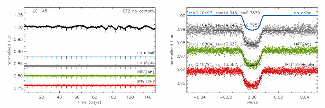
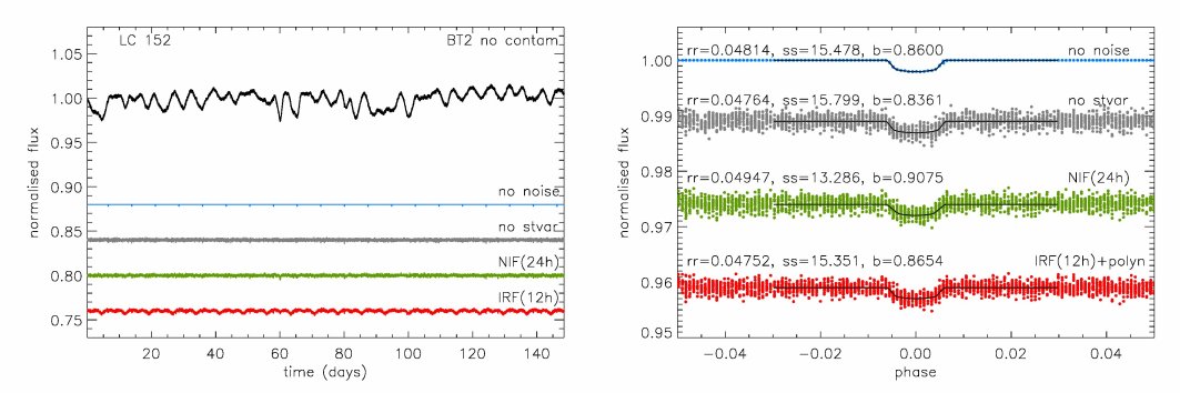
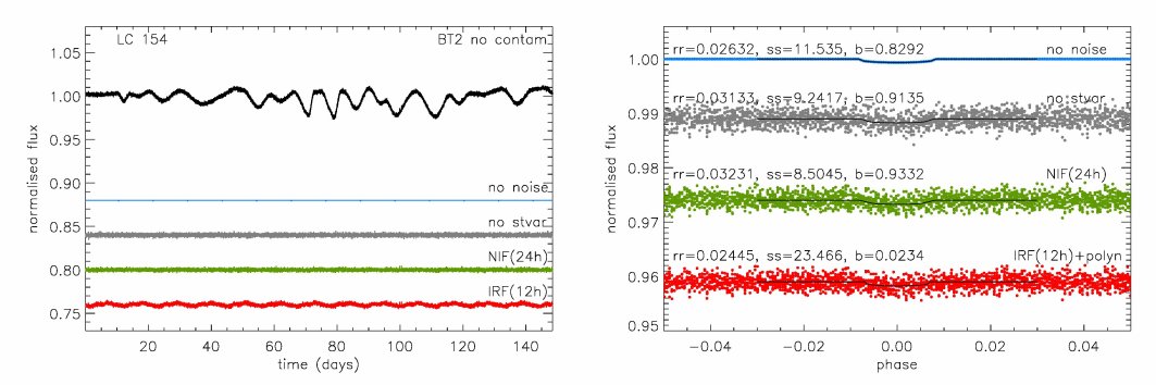
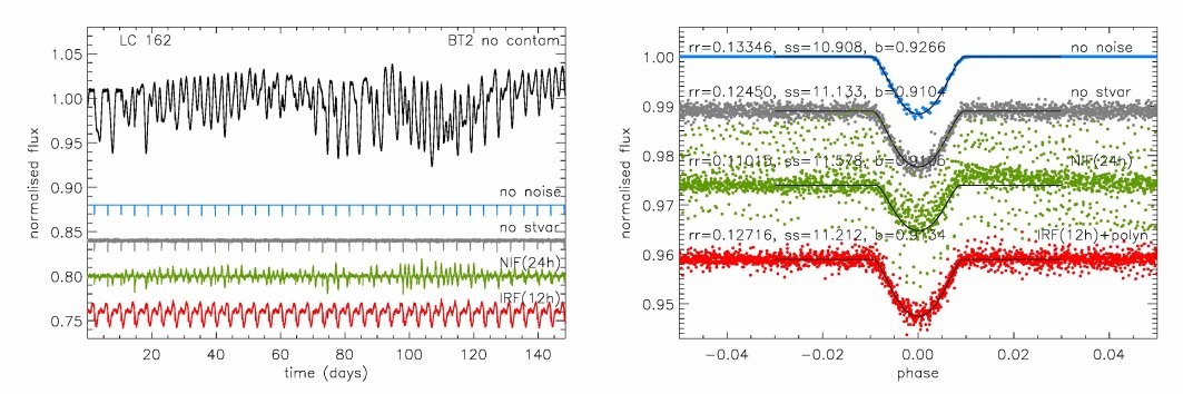
Figure 6: continued

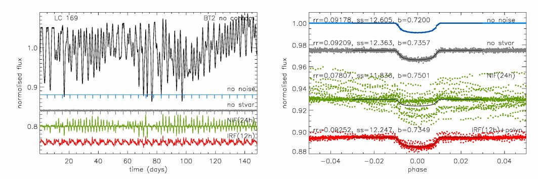
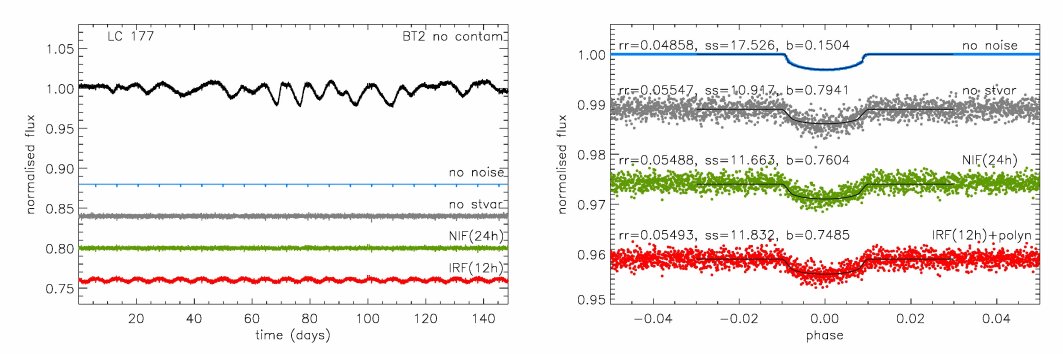
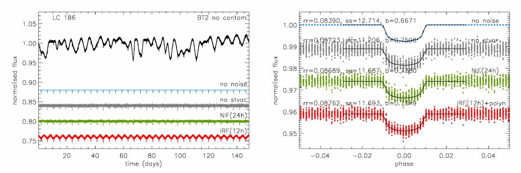
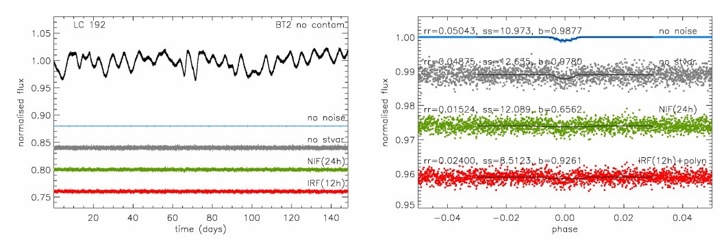
Figure 7: continued

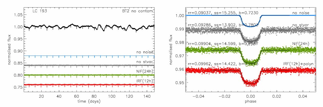
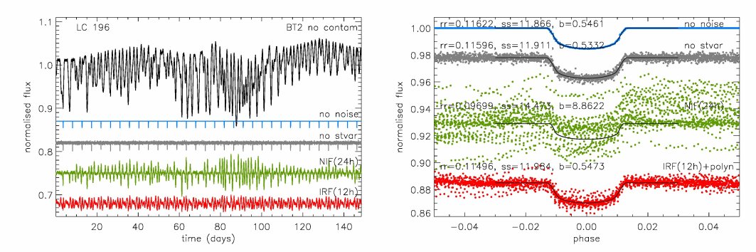
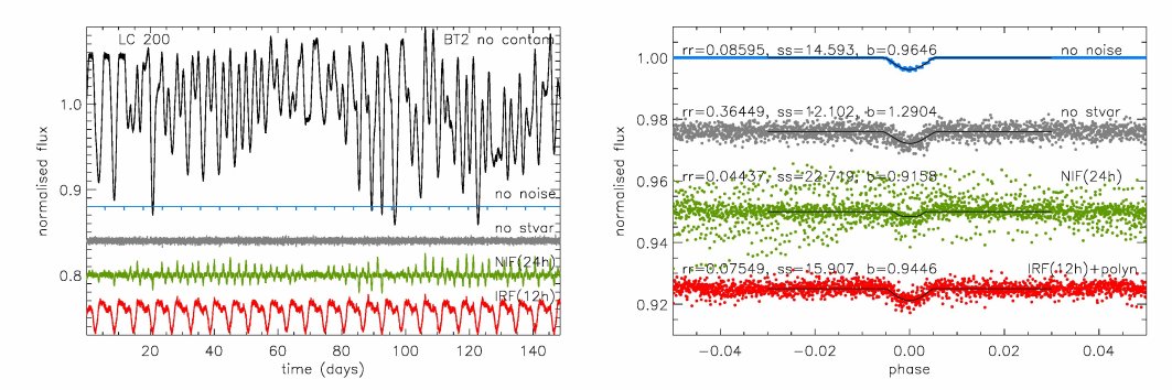
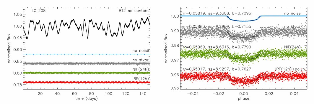
Figure 8: continued

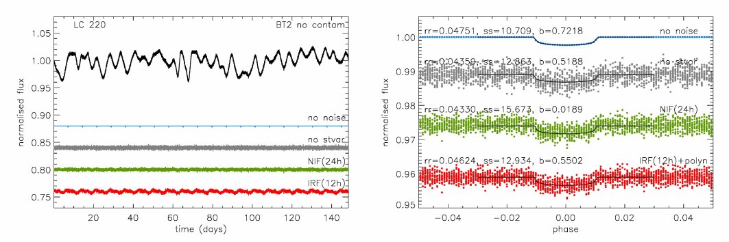
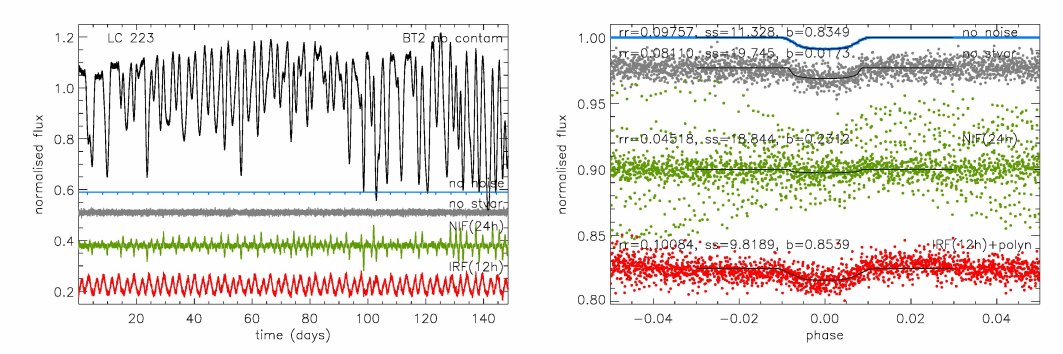
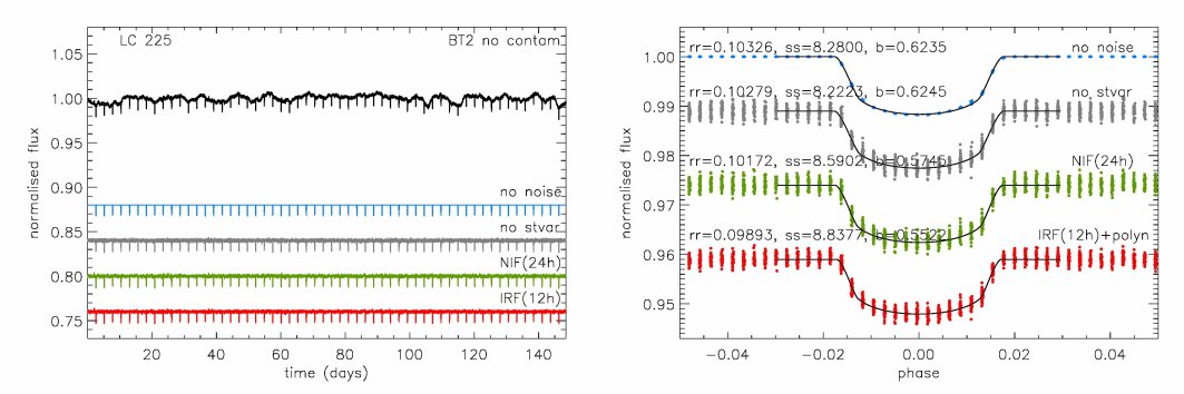
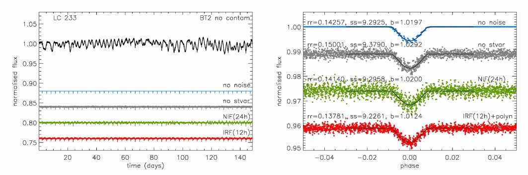
Figure 9: continued

Appendix B Best-fit parameters

Table 1: Transit parameters (transit depth $\delta$, total transit duration $d_{\rm e}$, and in-full transit duration $d_{\rm i}$) derived from trapezoidal fits to the light curves with transit signal only (‘no noise’), transit signal and instrumental noise only (‘no stvar’), the BT2 light curves filtered using the pre-detection nonlinear iterative filter (‘NIF’), and the same light curves filtered using post-detection iterative reconstruction filter (‘IRF’).

LC	period	$\delta$				$d_{\rm e}/P$				$d_{\rm i}$/P
	(days)	no noise	no stvar	NIF	IRF	no noise	no stvar	NIF	IRF	no noise	no stvar	NIF	IRF
126	4.576	0.00501	0.00495	0.00326	0.00504	0.0153	0.0153	0.0138	0.0153	0.0064	0.0064	0.0084	0.0079
131	6.880	0.00477	0.00469	0.00437	0.00448	0.0134	0.0121	0.0108	0.0121	0.0056	0.0017	0.0098	0.0098
133	8.128	0.00168	0.00161	0.00155	0.00160	0.0058	0.0058	0.0047	0.0057	0.0016	0.0010	0.0026	0.0015
135	3.733	0.00155	0.00148	0.00144	0.00152	0.0147	0.0147	0.0147	0.0147	0.0062	0.0062	0.0073	0.0090
145	5.557	0.00938	0.00949	0.00931	0.00923	0.0167	0.0153	0.0167	0.0167	0.0054	0.0064	0.0067	0.0086
152	7.360	0.00185	0.00185	0.00158	0.00176	0.0115	0.0125	0.0104	0.0115	0.0060	0.0065	0.0090	0.0071
154	10.987	0.00056	0.00065	0.00054	0.00061	0.0172	0.0172	0.0155	0.0237	0.0088	0.0038	0.0067	0.0051
162	4.171	0.00933	0.00922	0.00585	0.00894	0.0167	0.0167	0.0138	0.0167	0.0037	0.0037	0.0074	0.0070
169	5.195	0.00772	0.00770	0.00504	0.00769	0.0209	0.0209	0.0191	0.0209	0.0066	0.0066	0.0109	0.0107
177	7.339	0.00271	0.00267	0.00252	0.00260	0.0209	0.0209	0.0191	0.0209	0.0066	0.0046	0.0090	0.0107
186	4.373	0.00683	0.00679	0.00649	0.00690	0.0209	0.0209	0.0191	0.0209	0.0087	0.0087	0.0134	0.0127
192	3.915	0.00085	0.00102	0.00071	0.00076	0.0086	0.0094	0.0078	0.0078	0.0029	0.0023	0.0078	0.0070
193	6.763	0.00749	0.00747	0.00847	0.00858	0.0167	0.0167	0.0167	0.0167	0.0070	0.0070	0.0065	0.0086
196	4.608	0.01378	0.01384	0.00509	0.01288	0.0248	0.0248	0.0201	0.0248	0.0127	0.0127	0.0201	0.0175
200	5.995	0.00317	0.00313	0.00185	0.00311	0.0095	0.0095	0.0059	0.0086	0.0023	0.0023	0.0052	0.0038
208	4.064	0.00313	0.00301	0.00278	0.00302	0.0267	0.0267	0.0242	0.0267	0.0136	0.0136	0.0158	0.0162
220	7.253	0.00215	0.00212	0.00181	0.00216	0.0230	0.0250	0.0210	0.0230	0.0050	0.0030	0.0148	0.0140
223	5.237	0.00771	0.00736	0.00065	0.00761	0.0184	0.0184	0.0088	0.0200	0.0059	0.0059	0.0082	0.0102
225	2.613	0.01061	0.01053	0.01032	0.00998	0.0344	0.0344	0.0311	0.0344	0.0073	0.0073	0.0224	0.0174
233	3.083	0.00461	0.00460	0.00431	0.00459	0.0153	0.0153	0.0153	0.0153	0.0035	0.0035	0.0040	0.0049

Table 2: Star-planet parameters (planet to star radius ratio $R_{p}/R_{\star}$, system scale $a/R_{\star}$, and impact parameter $b$) derived from full transit fits. The columns corresponding to the 4 sets of light curves used in the fits are labelled as in Table LABEL:tab:trpara.

LC	period	$R_{p}/R_{\star}$				$a/R_{\star}$				$b$
	(days)	no noise	no stvar	NIF	IRF	no noise	no stvar	NIF	IRF	no noise	no stvar	NIF	IRF
126	4.576	0.0799	0.0800	0.0698	0.0817	12.27	12.09	13.14	11.89	0.862	0.870	0.858	0.872
131	6.880	0.0760	0.1687	0.0779	0.0749	15.64	9.64	10.65	12.30	0.825	1.058	0.893	0.873
133	8.128	0.1389	0.2836	0.0557	0.0642	17.70	15.59	20.99	20.65	1.074	1.233	0.961	0.979
135	3.733	0.0469	0.0369	0.0372	0.0393	10.00	20.34	20.62	16.75	0.916	0.422	0.397	0.676
145	5.557	0.1050	0.1044	0.1080	0.1079	14.35	14.24	13.34	13.38	0.788	0.795	0.822	0.820
152	7.360	0.0481	0.0476	0.0495	0.0475	15.48	15.80	13.29	15.35	0.860	0.836	0.908	0.865
154	10.987	0.0263	0.0313	0.0323	0.0245	11.54	9.24	8.50	23.47	0.829	0.914	0.933	0.023
162	4.171	0.1335	0.1245	0.1102	0.1272	10.91	11.13	11.58	11.21	0.927	0.910	0.911	0.913
169	5.195	0.0918	0.0921	0.0781	0.0925	12.61	12.36	11.84	12.25	0.720	0.736	0.750	0.735
177	7.339	0.0486	0.0555	0.0549	0.0549	17.53	10.92	11.66	11.83	0.150	0.794	0.760	0.749
186	4.373	0.0839	0.0872	0.0869	0.0876	12.71	11.21	11.69	11.69	0.667	0.760	0.738	0.735
192	3.915	0.0504	0.0488	0.0152	0.0240	10.97	12.64	12.09	8.51	0.988	0.978	0.656	0.926
193	6.763	0.0904	0.0929	0.0990	0.0996	15.26	13.90	14.60	14.42	0.723	0.780	0.759	0.764
196	4.608	0.1162	0.1160	0.0970	0.1150	11.87	11.91	14.47	11.98	0.546	0.533	0.000	0.547
200	5.995	0.0860	0.3645	0.0444	0.0755	14.59	12.10	22.72	15.91	0.965	1.290	0.916	0.945
208	4.064	0.0582	0.0588	0.0597	0.0592	9.33	9.30	8.63	8.93	0.710	0.716	0.780	0.763
220	7.253	0.0475	0.0436	0.0433	0.0462	10.71	12.86	15.67	12.93	0.722	0.519	0.019	0.550
223	5.237	0.0976	0.0811	0.0452	0.1008	11.33	19.75	18.84	9.82	0.835	0.017	0.231	0.854
225	2.613	0.1033	0.1028	0.1017	0.0989	8.28	8.22	8.59	8.84	0.624	0.625	0.575	0.552
233	3.083	0.1426	0.1500	0.1414	0.1378	9.29	9.38	9.30	9.23	1.020	1.029	1.020	1.012

Appendix C Contaminant flux

Table 3: Table of flux percentages coming from a contaminant star, for each of the BT2 light curve studied. Each light curves was corrected from the contaminant flux, before deriving transit and planet parameters. The fraction of flux coming from a contaminant star in each colour channel (CoRoT red, green and blue) was given in the parameter file used to build the BT2 light curves. For each light curve, the total contaminant flux was computed as the median of the sum of the contaminant fluxes in each colour channel, normalised by the median of the total flux.

LC	contaminant flux (%)	LC	contaminant flux (%)
105	0.2	177	0.6
110	0.1	186	0.3
126	2.2	192	0.8
131	90.6	193	13.1
133	0.2	196	0.9
135	0.1	200	3.3
145	2.3	208	1.8
152	0.3	220	1.9
154	1.9	223	77.4
162	0.1	225	0.6
165	91.1	233	0.6
169	0.5	236	1.4

References

- Adams et al. (2008) Adams E. R., Seager S., Elkins-Tanton L., 2008, ApJ, 673, 1160
- Aigrain et al. (2004) Aigrain S., Favata F., Gilmore G., 2004, A&A, 414, 1139
- Aigrain & Irwin (2004) Aigrain S., Irwin M., 2004, MNRAS, 350, 335
- Alonso et al. (2008) Alonso R., Aigrain S., Pont F., Mazeh T., the CoRoT Exoplanet Science Team 2008, ArXiv e-prints
- Alonso et al. (2008) Alonso R., Auvergne M., Baglin A., Ollivier M., Moutou C., Rouan D., Deeg H. J., Aigrain S., Almenara J. M., Barbieri M., Barge P., Benz W., et al 2008, A&A, 482, L21
- Auvergne et al. (2003) Auvergne M., Boisnard L., Buey J.-T. M., Epstein G., Hustaix H., Jouret M., Levacher P., Berrivin S., Baglin A., 2003, in Blades J. C., Siegmund O. H. W., eds, Future EUV/UV and Visible Space Astrophysics Missions and Instrumentation Vol. 4854 of Proc. SPIE, Corot-high-precision stellar photometry on a low earth orbit: solutions to minimize environmental perturbations. pp 170–180
- Bakos et al. (2007) Bakos G. Á., Noyes R. W., Kovács G., Latham D. W., Sasselov D. D., Torres G., Fischer D. A., Stefanik R. P., Sato B., Johnson J. A., Pál A., Marcy G. W., Butler R. P., Esquerdo G. A., Stanek K. Z., Lázár J., Papp I., et al 2007, ApJ, 656, 552
- Baraffe et al. (2008) Baraffe I., Chabrier G., Barman T., 2008, A&A, 482, 315
- Bonomo & Lanza (2008) Bonomo A. S., Lanza A. F., 2008, A&A, 482, 341
- Charbonneau et al. (2000) Charbonneau D., Brown T. M., Latham D. W., Mayor M., 2000, A&A, 529, L45
- Charbonneau et al. (2007) Charbonneau D., Winn J. N., Everett M. E., Latham D. W., Holman M. J., Esquerdo G. A., O’Donovan F. T., 2007, ApJ, 658, 1322
- Collier Cameron et al. (2007) Collier Cameron A., Wilson D. M., West R. G., Hebb L., Wang X.-B., Aigrain S., Bouchy F., Christian D. J., Clarkson W. I., Enoch B., Esposito M., Guenther E., Haswell C. A., Hébrard G. et a., 2007, MNRAS, 380, 1230
- Guillot (2005) Guillot T., 2005, Annual Review of Earth and Planetary Sciences, 33, 493
- Knutson et al. (2007) Knutson H. A., Charbonneau D., Noyes R. W., Brown T. M., Gilliland R. L., 2007, ApJ, 655, 564
- Kovács et al. (2005) Kovács G., Bakos G., Noyes R. W., 2005, MNRAS, 356, 557
- Lanza et al. (2004) Lanza A. F., Rodonò M., Pagano I., 2004, A&A, 425, 707
- Mandel & Agol (2002) Mandel K., Agol E., 2002, ApJL, 580, L171
- Mandushev et al. (2007) Mandushev G., O’Donovan F. T., Charbonneau D., Torres G., Latham D. W., Bakos G. Á., Dunham E. W., Sozzetti A., Fernández J. M., Esquerdo G. A., Everett M. E., Brown T. M., Rabus M., Belmonte J. A., Hillenbrand L. A., 2007, ApJL, 667, L195
- Moutou et al. (2007) Moutou C., Aigrain S., Almenara J., Alonso R., Auvergne M., Barge P., Blouin D., Borde P., Cabrera J., Carone L., Cautain R., Deeg H., Erikson A., Fressin F., Guis V., Leger A., et al 2007, in Afonso C., Weldrake D., Henning T., eds, Transiting Extrapolar Planets Workshop Vol. 366 of Astronomical Society of the Pacific Conference Series, Expected Performance of the CoRoT Planet Search from Light Curve Beauty Contests. pp 127–+
- Moutou et al. (2005) Moutou C., Pont F., Barge P., Aigrain S., Auvergne M., Blouin D., Cautain R., Erikson A. R., Guis V., Guterman P., Irwin M., Lanza A. F., Queloz D., Rauer H., Voss H., Zucker S., 2005, A&A, 437, 355
- Pál (2008) Pál A., 2008, MNRAS, 390, 281
- Seager et al. (2007) Seager S., Kuchner M., Hier-Majumder C. A., Militzer B., 2007, ApJ, 669, 1279
- Winn et al. (2007) Winn J. N., Holman M. J., Bakos G. Á., Pál A., Johnson J. A., Williams P. K. G., Shporer A., Mazeh T., Fernandez J., Latham D. W., Gillon M., 2007, AJ, 134, 1707
- Winn et al. (2008) Winn J. N., Holman M. J., Torres G., McCullough P., Johns-Krull C. M., Latham D. W., Shporer A., Mazeh T., Garcia-Melendo E., Foote C., Esquerdo G., Everett M., 2008, ApJ, submitted, arXiV:0804.4475