On mass hierarchies in orientifold vacua

Abstract:

We analyze the problem of the hierarchy of masses and mixings in orientifold realizations of the Standard Model. We find bottom-up brane configurations that can generate such hierarchies.

1 Introduction, motivation and scope

One of the biggest puzzles in the Standard Model (SM) is the origin and hierarchy of masses and mixings. When it comes to masses the scale of the problem is enormous: one needs to explain a range of masses that spans fifteen orders of magnitude between the mass of the lightest neutrino to the top. Moreover the patter of mixings is interesting. In the quark sector the first and second family mix strongly while all other mixings are small. In the lepton sector, all mixings measured so far are maximal. It seems to suggest that as we move up in mass mixings tend to become smaller.

There are several ideas on the origin of mass, the simplest being via a Higgs scalar that is responsible for electroweak symmetry breaking. This and related ideas are expected to be tested at LHC. There are fewer and definitely less successful ideas that are purported to explain the hierarchy of masses of the SM. They can be roughly lumped into four classes: radiative mechanisms, [1], texture zeros, [2, 3], family symmetries [4, 5, 6] and seesaw mechanisms, [7], although the classes are not completely disjoint. In particular texture zeros can be considered as a class of family symmetries as they are usually implemented via a discrete symmetry. Many of the ideas developed to deal with the mass hierarchy of th SM are reviewed in [8].

String theory has emerged as an arena for unifying interactions, in the last few decades. Finding the SM in a string theory vacuum has proved a difficult task especially when it comes to match to the SM pattern of masses. So far none of the early ideas on mass hierarchies has been successfully implemented in a string vacuum, although string inspired use of anomalous U(1)’s in that direction was advocated [9]. Recently, a simple implementation of the Froggatt-Nielsen idea was advocated in the context of F-theory, [10]. There have been however partial hierarchies in the SM spectrum that were successfully implemented like the top hierarchy and neutrino masses in the heterotic string using higher order couplings, [11, 12, 13, 14], or the third family and neutrino masses using large dimensions, [16].

Two perturbative landscapes of string theory vacua have monopolized attention in the past two decades. The first to be analyzed was the heterotic landscape deemed interesting because of its large and appealing gauge symmetry and the simplest structure of its perturbative expansion. Although a large set of vacua was found, some of them phenomenologically promising, several difficulties hampered the search for a SM-like vacuum, most of all the fact that the string theory input in vacuum construction (generalized geometry) is quite disjoint with the output (spectra, gauge groups, low energy interactions). At the same time, indications suggested that the heterotic string would need be in strong coupling in order for some effects to be compatible with data. At the same time, type-I theory emerged as a strong-coupling dual of the heterotic theory and SM-searches started to look in open string theory vacua.

Open string theory vacua, alias orientifolds, [17, 18, 19], provided a fresh new perspective in the search for the SM, [20]-[23]. They allowed a bottom-up approach, [24, 25] to building the SM, by utilizing the geometrized language offered by D-branes supporting the SM interactions and particles.

The algorithm can be described as follows. One first constructs a type II ground state, that involves a closed CFT describing the compactification. Then an appropriate orientifold projection is applied on the closed string sector. An open string sector is subsequently constructed by populating the allowed boundary states of the bulk CFT. This part of the algorithm should be thought of as inserting D-branes in the closed string vacuum in a way compatible with the 2d-dynamics. In particular the D-brane configuration is such that it guarantees local (as opposed to global) stability. At this stage one can engineer the gauge group and spectrum with rather milder constraints than those that are imposed at the end. Therefore a lot of the model building choices are decided early on. Moreover, in this context, one first constructs the SM family of branes, defined as the collection of boundary states that give rise to the chiral SM particles.

Finally, once the SM stack has been engineered to one’s satisfaction, the stringy, tadpole cancellation constraints are imposed. This can be done by adding in a modular fashion a “hidden sector”, ie. one or more brane stacks, that typically do not include light observable-hidden strings. The procedure stops when tadpoles are eventually canceled. This procedure has been algorithmized for a large set of RCFT building blocks, and used to provide large lists of SM-like orientifold vacua, [26, 27].

In [29] a class of orientifold vacua were studied, constructed from six copies of the second Gepner model (k=2). The original motivation was to study quasi-realistic vacua using CFT building blocks that are free CFTs. A very interesting feature of the vacua described in [29], was that the 3 SM families do not originate from the same D-branes. This has important consequences because of the generic presence of anomalous U(1) symmetries in orientifold vacua.

Anomalous U(1) symmetries are ubiquitous in orientifolds. It has been argued early on [24, 16], that any SM orientifold realization must have at least one and generically three anomalous U(1) symmetries, that make the most characteristic signature of orientifold vacua. Their phenomenological implications are diverse, [31]-[38].

Their most important property, that impacts importantly on the dynamics of the D-brane stack is that they provide numerous selection rules on the effective couplings. In particular, they may be responsible for the absence of the $\mu$-term, Yukawa couplings, baryon and lepton violating couplings etc. However, as anomalous U(1)’s are effectively broken as gauge symmetries, the selection rules they provide need qualification. As the breaking of the gauge symmetry happens via the mixing with RR forms, the global U(1) symmetry remains at this stage intact. There are two types of realizations of anomalous U(1) symmetries as global symmetries. If D-terms force charged fields to obtain vev’s then the global U(1) symmetry is broken. If on the other hand no vev’s are generated the anomalous U(1) global symmetry remain intact in perturbation theory.

However, the story must change beyond perturbation theory for two reasons. The first is that we do not expect exact (compact) global symmetries to survive in a gravitational theory. The second (in agreement with the first) is that there are always non-perturbative effects that violate the associated global symmetry. The argument is simple. A U(1) transformation involves a shift of RR field. The associated D-instanton effect which is charged under the same RR field (the Stuckelberg axion) will violate by definition the associated global U(1) symmetry. The effect is a D-instanton effect, whose field theory limit sometimes may admit a gauge instanton interpretation, [39]-[41]. Therefore, couplings a priori forbidden by anomalous U(1)’s can have three potential fates: (a) Be generated by a vev if the U(1)’ is broken by a charged scalar vev. (b) Be generated by an instanton effect, if there is an instanton with the requisite number of zero modes associated with a given coupling. (c) Remain zero as no vev or instanton can generate it.

In view of the discussion above we may appreciate why, segregating SM families on different D-branes may provide non-trivial selection rules of Yukawa couplings, generating eventually a hierarchy of masses. Indeed, in the vacuum studied in [29], for one of the quark family, no Yukawa couplings were allowed by the anomalous U(1) symmetries. Therefore, the Yukawa’s for this family, if generated at all, they must be generated by D-instantons and have therefore a natural exponential suppression with respect to the other two families.

A pertinent question at this stage is : are masses and mixings of the SM calculable in terms of a more fundamental theory (in the same sense that the energy spectrum of hydrogen is calculable) or are they “environmental parameters” that happen to have these values although there are other SM-like vacua where their values are different. Most physicists believe in the first possibility and it is fair to say that in the absence of convincing evidence for the second it is the most appealing one. However in the last few years there is evidence, in the context of string theory that many aspects of SM-like ground-states are not unique, but there is a large landscape of vacua with varying properties. We will not have anything to say on this issue that goes beyond our efforts in this paper. We do not pretend either to provide mechanisms that uniquely predict masses and mixings, but we explore how the associated hierarchies could be accommodated in orientifold vacua.

In this paper we will explore different effects that are prone to generate interesting hierarchies between fermion masses. Our scope is exploratory: there will be no concrete models of masses and mixings neither predictions/postdictions for experiment. The goal is to identify D-brane configurations that are promising when it comes to generating the fermion hierarchy. This is the problem we address in this paper. The next step will be to construct such interesting D-bane configurations.

There are several effects that can produce hierarchically different Yukawa-like couplings.

• Tree-level cubic Yukawa couplings. This is the generic case when such couplings are allowed. Their coefficient depends in general on several ingredients. It is always proportional to the ten-dimensional dilaton but also internal volumes, and other backgrounds fields (internal magnetic fields, fluxes) enter. They may be correlated with the associated gauge couplings if the fields participating come from overlapping D-branes. They may also be free of volumes if the branes intersect at points. Such variations are enough some times to explain the mass hierarchy inside a family. An example of this was presented in [16] in model B. There the tree-level Yukawa’s are such that once the top mass is fixed, the bottom and tau masses follow. It is important that such couplings are in the perturbative regime for the picture to be consistent. Another possibility that we study is that tree level couplings respect a discrete symmetry (that may be a local symmetry of the D-brane configuration). In such a case small variations of the closed string moduli may lead to an appropriate hierarchy of Yukawa couplings.

• Higher order couplings. These are couplings that appear beyond the cubic level. They necessarily involve more fields than the SM fields. These extra fields must obtain an expectation value in order for an effective Yukawa coupling to be generated. Then such couplings compared to the previous case carry an extra factor of $\left({\langle\phi\rangle\over M_{s}}\right)^{n}$ with $n$ a positive integer. Depending on the compactification the string scale may be replaced by a compactification scale. If $\langle\phi\rangle\ll M_{s}$ this generates a hierarchy in the associated Yukawa coupling. On the other hand the regime $\langle\phi\rangle\gg M_{s}$ is non-perturbative.

• D-Instanton-generated couplings. Such couplings violate the anomalous U(1) symmetries. They are suppressed by exponential instanton factors of the form $e^{-1/g}$ where $g$ is linearly related to the ten-dimensional coupling constant and depends also on the volume of the cycle the D-instanton is wrapped-on, as well as on other data (magnetic fields, fluxes etc). In the particular case of gauge instantons $g$ is the square of the associated gauge coupling. In the well-controlled regime, $g\ll 1$ and multi-instantons are suppressed. beyond the instanton-action factor, instanton-generated couplings carry a characteristic scale. This is determined by the string scale, or other volume factors affecting the world-volume factor of the D-instanton. Finally there is a one-loop determinant that is generically of order ${\cal O}$(1).

In this paper we will explore structures that allow exploiting a combination of the couplings above to generate mass and mixing hierarchies. One strategy will be the following:

1. We start from a D-brane configuration in the simplest bottom-up context, as first described in [24] and generally defined in [27]. It is described by a set of SM and (anomalous) U(1) charges for the SM particles, following the rules of D-brane engineering. In particular, generalized anomaly cancellation is imposed. All cubic Yukawa couplings allowed by the gauge symmetries are considered non-zero. We search and consider only bottom-up configurations that allow only one non-zero Yukawa coupling in each of the Up and Down quark $3\times 3$ mass matrices. The overall scale of masses is set by the vev’s of the two electroweak Higgses $H_{u}$ and $H_{d}$.

2. Apart from the SM particles and Higgses, one more scalar $\Phi$ will be advocated to help with the generation of higher order Yukawa couplings. Its vev will be selected to fit appropriate masses.

3. If a given Yukawa coupling is still zero, then a instanton contribution is advocated. Different Yukawa couplings generated by the same instanton (same violation of U(1) charges) will be considered to have the same exponential factor. This is stricter that what could really happen, as the same instanton can wrap two different cycles with very different volumes and can thus generate very different exponential factors. We will not use however this option in this paper. We will choose the exponential factors at will to reproduce the masses.

4. The rest of the coefficients in the mass matrices are dimensionless couplings that we will assume to be of the same order of magnitude and we will take them ad-hoc to vary in the interval [0.1,0.5]. A configuration will be deemed promising if it can reproduce the masses and mixings of the SM with dimensionless couplings in that range.

Such a strategy rests on a set of choices that could be otherwise. For example sometimes couplings can be much smaller than the range we choose. We do not pretend that our choices are universal. They provide however a general first assessment of D-brane vacua as to their ability to generate multiple scales for masses and mixings.

It should be noted that the previous context for generating the mass hierarchies of the SM, does not rest on family symmetries. As was first analyzed in [27], potential continuous family symmetries in the context of orientifold vacua are very different from those that have been explored in the QFT literature. The reason is simple: the doublet-triplet of quarks is constrained to have its two end-points on the SU(3) and SU(2) stacks of branes. Therefore the only extra charges it can carry are the $U(1)_{3}$ of the SU(3) charge (it is always present and it baryon number) and potentially the $U(1)_{2}$ of the SU(2) in the case of a complex weak stack (this U(1) is not present if the group is Sp(2)).

In the latter case of real weak stack, there is absolutely no difference between the three doublet-triplets, and they can carry no extra charges. In the first case of a complex weak stack, the doublet-triplets can be distinguished by the $U(1)_{2}$ charge that can take two possible values, $\pm 1$. Again at most one doublet-triplet can be different from the other two. No non-abelian charges are allowed in either case.

Even for discrete family symmetries the situation is different. In previous implementations such discrete symmetries come in two copies acting on the whole family on the left and on the right (see for example [4]). Here they typically come in one copy. A representative example are the discrete symmetries that appear when branes are stuck at orbifold singularities [25]. We will explore the impact of such symmetries on the mass spectrum later on in this paper.

Our results are as follows: in section 3.1 we found all possible textures of the mass matrices for the quarks and leptons for brane configurations with three, four and five stacks of branes. As stated above we aim to find among the possible orientifold vacua all models which give mass matrices with all the three scales. We found no such solutions in the case of three brane stacks.

For four brane stacks we found (in section 4) a vacuum in which the highest mass scale is related to Yukawa terms, the intermediate mass scale to instantons while the lowest scale to higher order terms. The CKM matrix computed for this model agrees with the experimental result. We also found a vacuum which satisfies the CKM constraint but only with Yukawas and higher order terms in the lepton mass matrices. In this model, there is no 1-1 correspondence between the fermion masses in each family and the Yukawa, higher order and instantonic terms. In the particular case of the KST model [29] we found a vacuum with only Yukawas and instantons which does not satisfy the CKM constraint.

Finally in the five stacks case we found a vacuum with three mass scales both in the quark and lepton sector which satisfies the CKM constraint.

The plan of our paper is as follows: In section 2 we give the description of D-brane configurations that successfully realize the SM spectrum. In section 3 we study the general form of the mass matrices for the quarks and leptons that is allowed in various configurations with three, four and five stacks of branes. In section 4 we concentrate on vacua with four and five branes with mass matrices with all the three scales. In section 5 we concentrate on an orientifold vacuum with a $Z_{3}$ discrete symmetry and we analyze the mass generation mechanism. In section 6 we present our conclusions.

In the appendix we provide more details about the three, four, and five brane stack vacua. We also provide the mass matrices for the quark, leptons and neutrinos of several bottom-up configurations.

2 Bottom-up description of D-brane configurations

A D-brane realization of the SM requires several stacks of branes. The minimum number of stacks is three [24] and all three-stack realizations were classified in [15]. Most common realizations utilize four stacks. There are also realizations with a higher number of stacks (an example is given in [28]).

All such configurations have in common a unitary stack of three branes (the “color” or A stack), a stack of two branes (the “weak” or B stack) and then various numbers of extra branes. In the simplest case they can be taken as single branes, but non-abelian stacks are also possible provided the associated gauge symmetry is eventually broken. Although this was explored in [27] we will not entertain this possibility here. We will only consider two extra stacks, C and D each made up of a single (complex) brane.

Gauge fields are described by open strings with both endpoints on the same stack and, generically, they give rise to Unitary, USp and SO groups. In particular the weak stack may have a U(2) or Sp(2) group. We will assume a U(2) group, and we will mention at the end differences in the Sp(2) case.

The rest of the SM particles are open strings attached on different (or the same) stack providing bi-fundamental (as well as symmetric or antisymmetric) representations. The hypercharge is a linear combination of the abelian factors of each stack. Typically the other linear combinations of the abelian factors are anomalous. These anomalies are canceled by the Green-Schwarz mechanism and by generalized Chern-Simons terms[30]. The anomalous U(1) gauge bosons are massive and their masses can vary between the string scale or much lower depending on appropriate volume factors [43].

The quark doublets $Q$ are described by strings with one end on the ‘A-stack and the other on the B-stack of branes. The quark singlets $U^{c},D^{c}$ are described either by strings which are stretched between stack A and the two extra U(1) C and D stacks. It is also possible to be generated by strings with both ends on the “color”-brane. In this case they transform in the antisymmetric representations of $SU(3)$ which is equivalent to the anti-fundamental. The lepton doublets $L$ are described by strings which are stretched between the B stack and the C,D stacks while the lepton singlets $E^{c}$ are described either by strings that are stretched between stacks C,D or by strings with both ends on the same single brane (B,C,D). In this case they transform in a symmetric representation of the corresponding abelian factor. The right-handed neutrinos $N^{c}$ being SM singlets are either described by strings attached on the SM-branes or they may come from the hidden sector of the model. In the first case they can be either stretched between the C,D stacks or they might have both ends on the B brane. In such a case they transform under the antisymmetric representation of the $SU(2)$ which is equivalent to the singlet.

3 Mass Matrices of the SM stack

Our main interest is to study the mass generation mechanism in orientifolds. As we mentioned above the SM particles are described by open strings whose ends are attached on various stacks of branes. In this case many Yukawa terms are forbidden due to the fact that they are not gauge invariant under the appropriate U(1) symmetries.

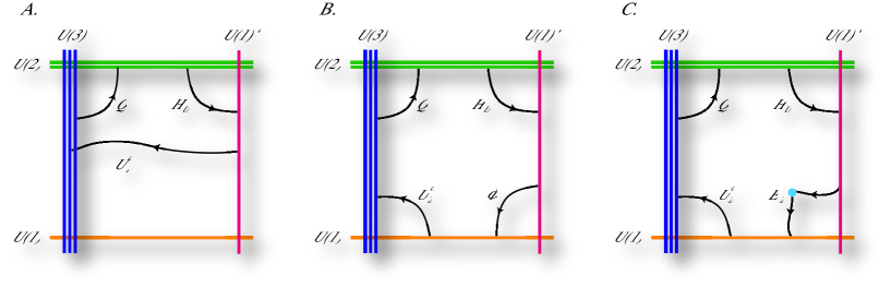
Figure 1: The three types of mass generating terms: The configuration A allows for a Yukawa term. However, in the B and C cases no Yukawa terms can be generated. In the B case there is a higher order term due to the presence of a field $\Phi$, while in the C case there is a contribution from an instanton term $E_{2}$.

An example of the four stacks’ case is sketched in figure 1, where $Q\sim(1,-1,0,0)$, $U^{c}_{1}\sim(-1,0,0,1)$, $U^{c}_{2}\sim(-1,0,1,0)$ and $H_{u}\sim(0,1,0,-1)$. The Yukawa term $QU^{c}_{1}H_{u}$ is uncharged under the four abelian factors and therefore is allowed while the term $QU^{c}_{2}H_{u}$ has charge $(0,0,1,-1)$ and thus forbidden. Such term could not contribute to the quark mass matrix. Here we will entertain the possibility that there are non-zero contributions for these mass matrix entries from higher-order terms and non-perturbative contributions.

Higher order terms must contain fields which are not present in the SM spectrum (with the exception of the neutrino mass terms). It is a generic feature of stringy spectra D-brane that additional non-chiral fields are present. In orientifolds some of them are important for generalized anomaly and tadpole cancellation. These fields can provide higher-order terms in the mass matrices. For example, we consider one of these additional field $\phi_{1}$ with charges $(0,0,-1,1)$, a SM singlet, originating from the non-chiral part of the spectrum. We also assume that $\phi_{1}$ acquires a non-zero vev $V_{\phi_{1}}$. In this case, the effective action contains a higher-order term of the form $QU^{c}_{2}H_{u}\phi_{1}$ that provides a quark mass term proportional to $V_{u}V_{\phi_{1}}/M_{s}$ where $V_{u}$ is the vev of $H_{u}$ and $M_{s}$ is the string scale. Since $V_{\phi_{1}}/M_{s}\lesssim 1$ in the perturbative regime, such a contribution is smaller than the leading Yukawa term. For the same reason, higher-order terms that are in principle allowed are suppressed by higher powers of $M_{s}$. Such scale differences in the mass matrices could be used to explain the hierarchy between the fermion masses.

When neither Yukawa nor higher order terms are allowed, we may consider non-perturbative contributions. D-instanton contributions give Yukawa couplings of the form $QU^{c}_{2}H_{u}~{}e^{-S_{I}}$ where $I$ denotes the type of instanton and the action, the coefficient $e^{-S_{I}}$ indicates the instanton action, $S_{I}$ is proportional to the internal volume the instanton brane wraps and it may also depend on other closed string moduli, [39, 40, 41]. For internal volumes a few times the string scale such contributions are exponentially suppressed. Summarizing, the following Yukawa-like terms can contribute to the mass matrix:

• Yukawa terms of the form $g_{i}QuH_{u}$

• Higher order terms of the form $g_{i}QuH_{u}\phi/M_{s}$ where $\phi$ a scalar field with zero hypercharge. Such terms are suppressed by the string scale $M_{s}$.

• Instanton terms of the form $g_{i}~{}QuH_{u}\times e^{-S_{I}}$. We will assume that $e^{-S_{I}}\lesssim 1$ so that we can neglect multi-instanton terms.

In all the previous terms the $g_{i}$’s are dimensionless coupling constants, which we assume to be of the same order ${\cal O}(1)$ and in the perturbative regime.

3.1 Mass Matrix Forms

In this section we study the general form of the mass matrices for the quarks and leptons that is allowed in various configurations with three, four and five stacks of branes.

We consider only vacua with two Higgs doublets $H_{u},~{}H_{d}$ which in particular could also accommodate the MSSM.

As mentioned in the introduction, in all orientifold vacua either all quark doublets are described by the same type of charges ($Q_{1}=Q_{2}=Q_{3}$) or one quark doublet is different from the other two $Q_{1}\neq Q_{2}=Q_{3}$. Therefore, as far as U(1) selection rules are concerned either all rows in the mass matrix will have the same type or one will be different from the other two.

After studying all possible bottom-up brane configurations we find that the resulting quark mass matrices are of the following form:

$$M_{Form-1} = ~{}\left(\begin{array}[]{lll}\cal X{}&\cal X{}&\cal X\\ \cal X{}&\cal X{}&\cal X\\ \cal X{}&\cal X{}&\cal X\\ \end{array}\right)$$ (4)

$$M_{Form-2} = ~{}\left(\begin{array}[]{l | ll}\cal X{}&\cal Y{}&\cal Y\\ \cal X{}&\cal Y{}&\cal Y\\ \cal X{}&\cal Y{}&\cal Y\\ \end{array}\right)~{}\sim~{}\left(\begin{array}[]{lll}\cal X{}&\cal X{}&\cal X\\ \hline\cr\cal Y{}&\cal Y{}&\cal Y\\ \cal Y{}&\cal Y{}&\cal Y\\ \end{array}\right)$$ (11)

$$M_{Form-3} = ~{}\left(\begin{array}[]{l | ll}\cal X{}&\cal Y{}&\cal Y\\ \hline\cr\cal Z{}&\cal U{}&\cal U\\ \cal Z{}&\cal U{}&\cal U\\ \end{array}\right)$$ (15)

$$M_{Form-4} = ~{}\left(\begin{array}[]{l | l | l}\cal X{}&\cal Y{}&\cal Z\\ \cal X{}&\cal Y{}&\cal Z\\ \cal X{}&\cal Y{}&\cal Z\\ \end{array}\right)$$ (19)

$$M_{Form-5} = ~{}\left(\begin{array}[]{l | l | l}\cal X{}&\cal Y{}&\cal Z\\ \hline\cr\cal U{}&\cal V{}&\cal W\\ \cal U{}&\cal V{}&\cal W\\ \end{array}\right)$$ (23)

where $\cal X,\cal Y,\cal Z,\cal U,\cal V,\cal W$ denotes terms of the same type, either Yukawa, higher-dimension or instantonic terms. While there can be only one kind of Yukawa and higher-dimension terms, in general there can be several different instantonic terms. For example there are vacua in which the $\cal Z$’s and the $\cal U$’s in (15) are all instantons but they are different from each other. Specific examples will be given in the following sections. Note that we consider as equivalent the two matrices (11) since they have the same hierarchy in their eigenvalues.

In the lepton sector, in addition to (4-23) we can also have vacua where all the entries in the mass matrix are different:

$$M_{Form-6} = ~{}\left(\begin{array}[]{l | l | l}\cal X{}&\cal Y{}&\cal Z\\ \hline\cr\cal U{}&\cal V{}&\cal W\\ \hline\cr\cal R{}&\cal S{}&\cal T\\ \end{array}\right)$$ (27)

Note that there are vacua in which the “weak” stack provides an $Sp(2)$ instead of $U(2)$. Since $Sp(2)$ is isomorphic to $SU(2)$ we do not have in this case the $U(1)$ factor associated to this stack of branes. Therefore, the quark doublets which are stretched between the A and the B branes have the same charges (+1,0,0) under the $U(1)_{A}\times U(1)_{C}\times U(1)_{D}$ and therefore the three doublets have all the same U(1) charges. In this case, the quark mass matrices can only have one of the forms: (4, 11, 19).

Below we give a classification of the D-brane realizations of the SM considering the possible form of the quark mass matrices. We restrict this analysis to the quark sector since in the lepton sector all mass matrix forms (4-27) are allowed in each realization.

Three Stacks: the $U(3)\times U(2)\times U(1)$ realizations

This setup has been first considered in detail in [15]. In this case there are two classes of vacua characterized by two different hypercharge embedding: $Y=-{1\over 3}Q_{\bf a}-{1\over 2}Q_{\bf b}$ and $Y={1\over 6}Q_{\bf a}+{1\over 2}Q_{\bf c}$ (the charge assignments for all the SM fields is given in appendix B.1).

• For $Y=-{1\over 3}Q_{\bf a}-{1\over 2}Q_{\bf b}$, the only possible form for both quark mass matrices $M_{U}$ and $M_{D}$ is (4).

• For $Y={1\over 6}Q_{\bf a}+{1\over 2}Q_{\bf c}$, there are two different possible charge assignments for the $d$-quarks allowing the corresponding mass matrix to be of the form either (4) or (11).

Four Stacks: the $U(3)_{A}\times U(2)_{B}\times U(1)_{C}\times U(1)_{D}$ realizations

In this case, there are seven different hypercharge embeddings (see appendix B.2).

• For $Y=-{1\over 3}Q_{\bf a}-{1\over 2}Q_{\bf b}+Q_{\bf d}$, both $M_{U},~{}M_{D}$ can be of the form (4, 11). This hypercharge embedding was identified as model A in [16].

• For $Y={2\over 3}Q_{\bf a}+{1\over 2}Q_{\bf b}+Q_{\bf c}$, $M_{U}$ can be of the form (4, 11) while $M_{D}$ can only be of the form (4). This hypercharge embedding was identified as model B in [16].

• For $Y={1\over 6}Q_{\bf a}+{1\over 2}Q_{\bf c}-{1\over 2}Q_{\bf d}$ (also known as the Madrid embedding, [45]), $M_{U}$ can be of the form (4-15) while $M_{D}$ can be of the form (4-23).

• For $Y={1\over 6}Q_{\bf a}+{1\over 2}Q_{\bf c}-{3\over 2}Q_{\bf d}$, $M_{U}$ can be of the form (4, 11) while $M_{D}$ can be of the form (4-15).

• For $Y=-{1\over 3}Q_{\bf a}-{1\over 2}Q_{\bf b}$, $M_{U}$ can only be of the form (4) while $M_{D}$ can be of the form (4, 11, 19).

• For the last two embeddings $Y=-{5\over 6}Q_{\bf a}-{Q_{\bf b}}-{1\over 2}Q_{\bf c}+{3\over 2}Q_{\bf d}$ and $Y={7\over 6}Q_{\bf a}+{Q_{\bf b}}+{3\over 2}Q_{\bf c}+{1\over 2}Q_{\bf d}$ both $M_{U},~{}M_{D}$ are of the form (4).

It is worth noting that in the Madrid embedding we get the highest number of different types of mass matrices. This is due to the fact that the C and D stacks contribute equally to the hypercharge allowing many alternative configurations. In the Madrid class of vacua it is possible to have charge assignments such that for the quarks, $Q_{1}\neq Q_{2}=Q_{3}$, $U_{1}\neq U_{2}=U_{3}$ and $D_{1}\neq D_{2}\neq D_{3}$. This in turn implies that both $M_{U}$ and $M_{D}$ can have three different kind of entries. In all the other vacua we considered, at least one of the following charge assignment, either $Q_{1}=Q_{2}=Q_{3}$ or $U_{1}=U_{2}=U_{3}$ or $D_{1}=D_{2}=D_{3}$, is realized.

Five Stacks: the $U(3)_{A}\times U(2)_{B}\times U(1)_{C}\times U(1)_{D}\times U(1)_{E}$ realizations

In this framework, we found 23 possible hypercharge embeddings. Among these embeddings, 12 of them have either $M_{U}$ or $M_{D}$ or both on them of the form (4). 8 of them have either $M_{U}$ or $M_{D}$ or both on them of the form (4) or (11). The remaining three are the most interesting ones where the mass matrices $M_{U}$ and $M_{D}$ can have at least three scales:

• For $Y={1\over 6}Q_{\bf a}+{1\over 2}Q_{\bf c}-{1\over 2}Q_{\bf d}-{3\over 2}Q_{\bf e}$ and $Y={1\over 6}Q_{\bf a}+{1\over 2}Q_{\bf c}-{1\over 2}Q_{\bf d}$, $M_{U}$ can be of the form (4-15) while $M_{D}$ can be of the form (4-23).

• For the “Madrid-like” 5 stacks extension: $Y={1\over 6}Q_{\bf a}+{1\over 2}Q_{\bf c}+{1\over 2}Q_{\bf d}+{1\over 2}Q_{\bf e}$ where all single branes democratically contribute with a factor 1/2 to the hypercharge, both $M_{U}$ and $M_{D}$ can be of the form (4-23).

Note that as in the four-stacks’ case, the Madrid-like embedding gives the highest number of different mass matrices. In addition, only in this context we can have both $M_{U},~{}M_{D}$ of the form (23).

4 Vacua with 3-scales in all fermion mass matrices

In each of the SM mass matrices for the quarks and leptons there is a large hierarchy. In this work, we want to explore the possibility that the different scales are related to the three different types of possible Yukawa-like terms. Therefore, we consider vacua where the quark and lepton mass matrices have the forms (15-27). This excludes all three stack constructions (B.1) as well as all four stack constructions (B.2) apart from a subclass of the “Madrid” vacua (B.2).

In order to satisfy the above requirements, the vacuum should contain one quark doublet different from the other two (say $Q_{1}\neq Q_{2}=Q_{3}$) as well as a different right-handed $U^{c}$ and $D^{c}$ from the other two (say $U^{c}_{1}\neq U^{c}_{2}=U^{c}_{3}$ and $D^{c}_{1}\neq D^{c}_{2}=D^{c}_{3}$). This choice ensures the “3-scales” in the quark mass matrices and fixes all the quarks since each of them has only two possible descriptions. For the choice of leptons we have some more freedom since each lepton doublet and singlet can get several different charge assignments (as can be seen in (B.2)). A subclass of the Madrid vacua that satisfy our requirements is:

$$Q_{1}~{}~{}~{}~{}:~{}(~{}~{}1,+1,~{}~{}0,~{}~{}0)~{}~{}~{},~{}~{}Q_{2},Q_{3}~{}:~{}(~{}~{}1,-1,~{}~{}0,~{}~{}0)$$

$$U^{c}_{1}~{}~{}~{}~{}:~{}(-1,~{}~{}0,-1,~{}~{}0)~{}~{}~{},~{}~{}U^{c}_{2}~{}U^{c}_{3}~{}:~{}(-1,~{}~{}0,~{}~{}0,-1)$$

$$D^{c}_{1}~{}~{}~{}~{}:~{}(-1,~{}~{}0,+1,~{}~{}0)~{}~{}~{},~{}~{}D^{c}_{2}~{}D^{c}_{3}:~{}(-1,~{}~{}0,~{}~{}0,+1)$$

$$L^{c}_{1}~{}~{}~{}~{}:~{}(~{}~{}0,~{}~{}1,-a,a-1)~{},~{}L^{c}_{2}~{}L^{c}_{3}~{}:~{}(~{}~{}0,~{}~{}1,-b,b-1)$$

$$E^{c}_{1}~{}~{}~{}~{}:~{}(~{}~{}0,~{}~{}0,~{}~{}c,~{}~{}d)~{}~{}~{},~{}~{}E^{c}_{2}~{}~{}~{}~{}~{}:~{}(~{}~{}0,~{}~{}0,~{}~{}e,~{}~{}f)~{}~{},~{}~{}E^{c}_{2}~{}:~{}(~{}~{}0,~{}~{}0,~{}~{}g,~{}~{}h)$$

$$N^{c}_{1,2,3}:~{}(~{}~{}0,\pm 2,~{}~{}0,~{}~{}0)$$ (28)

where $a,b=(0,1)$ and $c,d,e,f,g,h=(0,1,2)$ with the constraint $|c+d|=|e+f|=|g+h|=2$. Notice that the lepton doublets can all have different charge assignments in a single vacuum. The two MSSM Higgses are described by

$$H_{u}~{} : ~{}(0,-1,+1,0)$$

$$H_{d}~{} : ~{}(0,-1,-1,0)$$ (29)

and we consider two additional scalars with zero hypercharge $\phi_{1}$ and $\phi_{2}$, coming from the non chiral part of the spectrum:

$$\phi_{1}~{} : ~{}(0,0,-1,+1)$$

$$\phi_{2}~{} : ~{}(0,0,+1,-1)~{}.$$ (30)

The brane configurations that we consider here are subject to two constraints: the spectrum must match that of the MSSM in the chiral sense, with chirality defined with respect to $SU(3)\times SU(2)\times U(1)$. Furthermore all cubic anomalies in each factor of the full Chan-Paton group must cancel. This must be true because we want to be able to cancel tadpoles, and tadpole cancelation imposes cubic anomaly cancelation (mixed anomalies are canceled by the generalized Green-Schwarz mechanism). The tadpoles are usually canceled by adding hidden sectors, which adds new massless states to the spectrum. These are non-chiral and thus they do not alter the anomaly cancelation mechanism in the MSSM sector. As described in [27] the cubic anomaly cancelation conditions that are derived from tadpole cancelation are the usual ones for the non-abelian subgroups of $U(N)$, $N>2$. Vectors contribute 1, symmetric tensors $N+4$ and anti-symmetric tensors $N-4$, and conjugates contribute with opposite signs. But the same condition emerges even if $N=1$ and $N=2$. This means that for example a combination of three vectors and an anti-symmetric tensor is allowed in a $U(1)$ factor. This is counter-intuitive, because the anti-symmetric tensor does not even contribute massless states, so that one is left with just three chiral massless particles, all with charge 1. The origin of the paradox is that it is incorrect to call this condition “anomaly cancelation” if $N=1$ and $N=2$ and if chiral tensors are present. It is simply a consequence of tadpole cancelation; the anomaly introduced by the three charge 1 particles is factorizable, and canceled by the Green-Schwarz mechanism.

Using the above constraints we finally get eight vacua which are anomaly free and with 3 different kind of terms in the quark and lepton mass matrices. Inserting the values of table 1 in (28) we get the different charge assignments for each vacuum.

In the appendix F we provide a complete description of the mass matrices.

vacuum	$~{}~{}a~{}~{}$	$~{}~{}b~{}~{}$	$~{}~{}c~{}~{}$	$~{}~{}d~{}~{}$	$~{}~{}e~{}~{}$	$~{}~{}f~{}~{}$	$~{}~{}g~{}~{}$	$~{}~{}h~{}~{}$
1:	1	1	0	2	1	1	2	0
2:	0	1	0	2	2	0	2	0
3:	1	0	0	2	1	1	1	1
4:	1	0	1	1	2	0	2	0
5:	0	1	0	2	0	2	1	1
6:	0	1	1	1	1	1	2	0
7:	1	0	0	2	0	2	2	0
8:	0	0	0	2	1	1	2	0

Table 1: The eight consistent vacua with 3-scales in each of the mass matrices of the quarks and leptons.

4.1 Vacuum 1: $a=1,~{}b=c=e=h=0,~{}d=f=g=2$.

As an example, we choose the first vacuum in table 1. The corresponding mass matrices for the quarks have the form:

$$M_{U} = V_{u}~{}\left(\begin{array}[]{lll}g_{1}{}&g_{2}v_{\phi_{1}}&g_{3}v_{\phi_{1}}\\ g_{4}E_{1}&g_{5}E_{2}&g_{6}E_{2}\\ g_{7}E_{1}&g_{8}E_{2}&g_{9}E_{2}\\ \end{array}\right)$$ (34)

$$M_{D} = V_{d}~{}\left(\begin{array}[]{lll}q_{1}{}&q_{2}v_{\phi_{2}}&q_{3}v_{\phi_{2}}\\ q_{4}E_{1}&q_{5}E_{3}&q_{6}E_{3}\\ q_{7}E_{1}&q_{8}E_{3}&q_{9}E_{3}\\ \end{array}\right)$$ (38)

where $v_{\phi_{1}}=V_{\phi_{1}}/M_{s}$, ${v_{\phi}}_{2}=V_{\phi_{2}}/M_{s}$ and $E_{i}=e^{-Vol_{I_{i}}I_{i}}$ are the dimensionless instantons. These two matrices have the form (15) where $\cal X$ is a Yukawa term, $\cal Y$’s are higher terms and the $\cal Z$’s and the $\cal U$’s are instantons $E_{1}$ and $E_{2}$ respectively. The above matrices are the same for all the eight vacua in (28). The mass matrices for the leptons and neutrinos change form and in this specific vacuum we have:

$$M_{L} = V_{d}~{}\left(\begin{array}[]{lll}l_{1}E_{4}&l_{2}v_{\phi_{1}}&l_{3}{}\\ l_{4}E_{4}&l_{5}v_{\phi_{1}}&l_{6}{}\\ l_{7}E_{4}&l_{8}v_{\phi_{1}}&l_{9}{}\\ \end{array}\right)$$ (42)

$$M_{N} = \left(\begin{array}[]{llllll}0&0&0&g_{11}V_{u}E_{1}&g_{12}V_{u}E_{1}&g_{13}V_{u}E_{1}\\ 0&0&0&g_{21}V_{u}E_{1}&g_{22}V_{u}E_{1}&g_{23}V_{u}E_{1}\\ 0&0&0&g_{31}V_{u}E_{1}&g_{32}V_{u}E_{1}&g_{33}V_{u}E_{1}\\ g_{11}V_{u}E_{1}&g_{21}V_{u}E_{1}&g_{31}V_{u}E_{1}&q_{11}M_{s}E_{5}&q_{12}M_{s}E_{5}&q_{13}M_{s}E_{5}\\ g_{12}V_{u}E_{1}&g_{22}V_{u}E_{1}&g_{32}V_{u}E_{1}&q_{21}M_{s}E_{5}&q_{22}M_{s}E_{5}&q_{23}M_{s}E_{5}\\ g_{13}V_{u}E_{1}&g_{23}V_{u}E_{1}&g_{33}V_{u}E_{1}&q_{31}M_{s}E_{5}&q_{32}M_{s}E_{5}&q_{33}M_{s}E_{5}\end{array}\right)$$ (49)

where $g_{i},~{}q_{i},~{}l_{i}$ and $g_{ij},~{}q_{ij}$ are dimensionless couplings assumed to be of the same order. It is easy to check that neither Yukawa nor Majorana terms are present in the neutrino mass matrix for the vacua of table 1. The only way to get such terms is by instantonic contributions $E_{1}$ and $E_{5}$. The $E_{1}$ are the same dimensionless instantonic contribution that also appear in the $U$-quark mass matrix (34).

The parameters of our vacuum are evaluated by equating the eigenvalues of all the mass matrices to the running values of the quark, lepton and neutrino masses at various scales. If the vacuum is supersymmetric, the low-energy effective action has softly broken Susy and therefore all couplings run logarithmically. In the non-supersymmetric case, some other solution to the hierarchy problem must be invoked so that couplings run logarithmically.

The values of the quarks, leptons and neutrino masses at various scales have been computed in the MSSM framework [48]. Since there are several unknown parameters in each mass matrix, we fix some of them and we solve the system for the remaining ones. We perform this task by requiring that all the dimensionless couplings must be of the same order.

For example, in the $M_{U}$ matrix, all entries in the $2\times 2$ matrix:

$$\left(\begin{array}[]{ll}g_{5}~{}E_{2}&g_{6}~{}E_{2}\\ g_{8}~{}E_{2}&g_{9}~{}E_{2}\\ \end{array}\right)$$ (53)

should be of the same order due to our constraint. This requirement is not in general satisfied in the MSSM. In our analysis we explore three possibilities for the value of the string scale: $M_{s}=1$ TeV, $M_{s}=10^{12}$ GeV and at $M_{s}=\Lambda_{GUT}=2\times 10^{16}$ GeV scale.

Here we give a brief description of the strategy we followed in order to determine the values of the vev’s and instantons. Each mass matrix entry is parametrized as a product of a coupling $g_{i}$ with one of the relevant parameter, namely a plain Yukawa term, a vev or an instanton. We fix some of these parameters to reproduce for example the masses of the heaviest quarks. The remaining parameters are fixed by imposing the equality of the mass matrices eigenvalues with the experimental values. The couplings $g_{i}$ are used as fine tuning parameters varying their values at random in a small interval $[0.1,0.6]$.

For the present vacuum (as well as for the second and third in table 1) we were able to find solutions where

$$V_{u}\sim m_{t},~{}V_{d}\sim m_{b}$$

$$E_{1}\sim E_{2}\sim m_{c}/m_{t}$$

$$E_{3}\sim E_{4}\sim m_{s}/m_{b}$$

$$v_{\phi_{1}}\sim m_{u}/m_{t}$$

$$v_{\phi_{2}}\sim m_{d}/m_{b}$$ (54)

where $m_{i}$ are the masses of the corresponding quarks, and all couplings $|g_{i}|$, $|q_{i}|$, $|l_{i}|$, $|g_{ij}|$, $|q_{ij}|$ are within the range $[0.1,0.6]$.

As we mentioned before, in order to get the tiny neutrino masses we have to implement the seesaw mechanism. The main idea of this mechanism can be sketched in a simple case of a $2\times 2$ matrix:

$$M_{N} \sim \left(\begin{array}[]{ll}0&m\\ m&M\end{array}\right)$$ (57)

where $M\gg m$. This matrix has one eigenvalue which is proportional to $M$ while the other one is proportional to $m^{2}/M$. The previous result can be easily extended in our case of the $6\times 6$ neutrino mass matrix (49). In this matrix, all the entries of the off diagonal $3\times 3$ submatrices, module the couplings $g_{ij}$, are fixed by the previous requirements (54) giving mass scales that range from $10^{-1}-10^{3}$ MeV. Therefore, to obtain the tiny neutrino mass the scale of the lower block diagonal $3\times 3$ submatrix must be of order of the highest scale of the theory, i.e. $M_{s}$. Indeed, following the same procedure we used in the quark and lepton sector, we find at different scales:

$${\rm 1~{}TeV~{}scale}~{}~{} : ~{}~{}~{}~{}E_{5}\sim 0.654$$

$${\rm 10^{12}~{}GeV~{}scale}~{}~{} : ~{}~{}~{}~{}E_{5}\sim 0.754$$

$${\rm\Lambda_{GUT}~{}scale}~{}~{} : ~{}~{}~{}~{}E_{5}\sim 2.5\times 10^{-7}$$ (58)

which are in the expected range.

Mixing Matrices

Using the above values for the couplings and vev’s, we can proceed and evaluate the Cabbibo - Kobayashi - Maskawa Matrix (CKM). For the above vacuum, the matrix is:

$${\rm CKM(1TeV)} = \left(\begin{array}[]{lll}0.970&0.240&0.007\\ 0.240&0.970&0.013\\ 0.010&0.011&0.999\end{array}\right)$$ (62)

that has to be compared with the experimental data [53]:

$${\rm CKM(Data)} = \left(\begin{array}[]{rrr}0.97419\pm 0.00022&0.2257\pm 0.0010&~{}~{}~{}~{}~{}0.00359\pm 0.00016\\ 0.2256\pm 0.0010&~{}~{}~{}~{}~{}0.97334\pm 0.00023&0.0415\pm 0.001\\ 0.00874^{+0.00026}_{-0.00037}&0.0407\pm 0.0010&0.999133^{+0.000044}_{-0.000043}\end{array}\right)$$ (66)

Similarly, we evaluate the neutrino mixing matrix:

$${\rm U_{Neutrino~{}Mixing}} = \left(\begin{array}[]{rrr}-0.42-0.23i&-0.53+0.38i&-0.19-0.54i\\ 0.69-0.21i&-0.34+0.10i&-0.55+0.17i\\ 0.20-0.44i&0.65&-0.16-0.55i\end{array}\right)$$ (71)

The mixing matrices at $10^{12}{\rm GeV}$ and $\Lambda_{GUT}$ are:

$${\rm CKM}(10^{12}{\rm GeV})=\left(\begin{array}[]{rrr}0.974&0.221&0.020\\ 0.221&0.975&0.003\\ 0.019&0.007&0.999\end{array}\right)$$ (75)

$${\rm U_{Neutrino~{}Mixing}}(10^{12}{\rm GeV})=\left(\begin{array}[]{rrr}0.56-0.47i&0.05-0.01i&0.66+0.06i\\ -0.47+0.36i&0.42-0.25i&0.61+0.09i\\ 0.29-0.01i&0.86&-0.31-0.24i\end{array}\right)~{}~{}~{}~{}~{}$$ (79)

at $M_{s}=10^{12}$ GeV, and

$${\rm CKM}(\Lambda_{GUT})=\left(\begin{array}[]{rrr}0.971&0.235&0.017\\ 0.235&0.971&0.002\\ 0.017&0.001&0.999\end{array}\right)$$ (83)

$${\rm U_{Neutrino~{}Mixing}}(\Lambda_{GUT})=\left(\begin{array}[]{rrr}0.82&0.11-0.44i&0.20+0.24i\\ -0.38-0.32i&0.56-0.12i&0.33+0.54i\\ 0.19+0.14i&-0.05+0.67i&0.69\end{array}\right)~{}~{}~{}~{}~{}$$ (87)

at $M_{s}=\Lambda_{GUT}$.

4.2 Vacuum 4: $a=c=d=1,~{}b=f=h=0,~{}e=g=2$.

As we mentioned before, among the eight possible vacua in table 1 we were able to find solutions of the form (54) only for the first three models. Here we concentrate on the fourth model in table 1, i.e. $a=c=d=1,~{}b=f=h=0,~{}e=g=2$.

In this case the corresponding quark mass matrices $M_{U},~{}M_{D}$ have the form given in (34), while the mass matrices for the leptons and neutrinos have a different form:

$$M_{L} = V_{d}~{}\left(\begin{array}[]{lll}l_{1}v_{\phi_{2}}&l_{2}{}&l_{3}{}\\ l_{4}{}&l_{5}v_{\phi_{1}}&l_{6}v_{\phi_{1}}\\ l_{7}{}&l_{8}v_{\phi_{1}}&l_{9}v_{\phi_{1}}\\ \end{array}\right)$$ (91)

where $l_{i}$ are dimensionless couplings assumed to be of the same order and:

$$M_{N} \sim \left(\begin{array}[]{llllll}0&0&0&g_{11}V_{u}E_{1}&g_{12}V_{u}E_{1}&g_{13}V_{u}E_{1}\\ 0&0&0&g_{21}V_{u}E_{2}&g_{22}V_{u}E_{2}&g_{23}V_{u}E_{2}\\ 0&0&0&g_{31}V_{u}E_{2}&g_{32}V_{u}E_{2}&g_{33}V_{u}E_{2}\\ g_{11}V_{u}E_{1}&g_{21}V_{u}E_{2}&g_{31}V_{u}E_{2}&q_{11}M_{s}E_{4}&q_{12}M_{s}E_{4}&q_{13}M_{s}E_{4}\\ g_{12}V_{u}E_{1}&g_{22}V_{u}E_{2}&g_{32}V_{u}E_{2}&q_{21}M_{s}E_{4}&q_{22}M_{s}E_{4}&q_{23}M_{s}E_{4}\\ g_{13}V_{u}E_{1}&g_{23}V_{u}E_{2}&g_{33}V_{u}E_{2}&q_{31}M_{s}E_{4}&q_{32}M_{s}E_{4}&q_{33}M_{s}E_{4}\end{array}\right)$$ (98)

where $E_{1},~{}E_{2}$ are the same dimensionless instantonic contributions that also appear in the $U$-quark mass matrix (34).

We can repeat the same procedure and evaluate the values of the vev’s and instantons at various scales. In details we fix the vev’s of the two Higges $V_{u},~{}V_{d}$ to the values of the masses of the heaviest quarks $m_{\tau},m_{b}$ at this scale. This choice implies that the higher mass scale comes from the Yukawa terms. In order to evaluate the values for the rest of the unknown parameters, we choose at random the norm of the couplings $|g_{i}|,~{}|q_{i}|,~{}|l_{i}|,~{}|g_{ij}|,~{}|q_{ij}|$ in a small interval of $[0.1,0.6]$ and we solve the systems equating the three eigenvalues of each matrix with the masses of the relevant particles.

To summarize we have computed these values at the scales of 1 TeV, $10^{12}$ GeV and at GUT scale. The results are given in the following table:

(103)

Notice that we have three scales: one related to the Yukawa terms $V_{u},~{}V_{d}$, one related to the higher order terms $v_{\phi_{1}},~{}v_{\phi_{2}}$ and one related to the instanton terms $E_{1},~{}E_{2},~{}E_{3}$.

The $E_{4}$ instanton is much higher than the other instanton contributions because it appears in the Majorana part (lower right $3\times 3$ submatrix) of the seesaw neutrino mass matrix (98).

Mixing Matrices

Using the above values for the couplings and vev’s, we can proceed and evaluate the Cabbibo - Kobayashi - Maskawa Matrix (CKM). For the above vacuum, the matrix is:

$${\rm CKM(1TeV)} = \left(\begin{array}[]{lll}0.97323&0.22979&0.00300\\ 0.22971&0.97235&0.04200\\ 0.00673&0.04157&0.99911\end{array}\right)$$ (107)

that is in agreement with data (LABEL:CKMdata). Similarly, we evaluate the neutrino mixing matrix:

$${\rm U_{Neutrino~{}Mixing}} = \left(\begin{array}[]{rrr}0.484+0.118i&0.166-0.687i&-0.486-0.117i\\ 0.294+0.643i&0.001&0.295+0.642i\\ -0.5i&0.707&0.5i\end{array}\right)$$ (111)

For the rest of the scales, the mixing matrices are:

$${\rm CKM}(10^{12}{\rm GeV})=\left(\begin{array}[]{rrr}0.992&0.111&0.038\\ 0.114&0.835&0.538\\ 0.028&0.538&0.842\end{array}\right)$$ (115)

$${\rm U_{Neutrino~{}Mixing}}(10^{12}{\rm GeV})=\left(\begin{array}[]{rrr}0.995{}&0.04-0.04i&0.05+0.05i\\ -0.076i{}&0.74+0.24i&-0.61+0.06i\\ -0.054{}&0.56+0.25i&0.78\end{array}\right)~{}~{}~{}~{}~{}$$ (119)

at $M_{s}=10^{12}$ GeV, and

$${\rm CKM}(\Lambda_{GUT})=\left(\begin{array}[]{rrr}0.973&0.228&0.003\\ 0.228&0.972&0.042\\ 0.006&0.041&0.999\end{array}\right)$$ (123)

$${\rm U_{Neutrino~{}Mixing}}(\Lambda_{GUT})=\left(\begin{array}[]{rrr}-0.43-0.11i{}&0.76-0.06i{}&0.05-0.46i\\ -0.07-0.34i{}&-0.18-0.59i{}&0.70\\ 0.82{}&0.13-0.11i{}&0.02-0.54i\end{array}\right)~{}~{}~{}~{}~{}$$ (127)

at $M_{s}=\Lambda_{GUT}$.

4.3 The KST vacua

In this section we consider a different vacuum which was studied in [29]. This is a (almost) free-field vacuum with tadpole cancellation. The gauge group is $U(3)\times Sp(2)\times U(1)\times U(1)^{\prime}$ times an additional $SU(2)$ coming from the hidden sector of the vacuum. The massless spectrum contains:

(134)

Notice that the two right-handed neutrinos $N^{c}_{2},~{}N^{c}_{3}$ come from the hidden sector and in particular, they are described by an antisymmetric and it’s conjugate representation of the hidden $SU(2)$ sector. The two MSSM Higgses are described by

$$H_{u}~{} : ~{}(0,-1,+1,0)$$

$$H_{d}~{} : ~{}(0,+1,-1,0)~{}.$$ (135)

In this vacuum, an instanton $E_{1}$ and its conjugate $E_{1}^{*}$ are needed in order to generate the relevant mass terms for the fermions. The form of this instantons are:

$$E_{1}~{} : ~{}(0,0,-1,+1)$$

$$E_{1}^{*}~{} : ~{}(0,0,+1,-1)$$ (136)

The quark mass matrices for this vacuum are given by:

$$M_{U} = V_{u}~{}\left(\begin{array}[]{lll}g_{1}{}&g_{2}{}&g_{3}E_{1}^{*}\\ g_{4}{}&g_{5}{}&g_{6}E_{1}^{*}\\ g_{7}{}&g_{8}{}&g_{9}E_{1}^{*}\\ \end{array}\right)$$ (140)

$$M_{D} = V_{d}~{}\left(\begin{array}[]{lll}q_{1}{}&q_{2}{}&q_{3}E_{1}\\ q_{4}{}&q_{5}{}&q_{6}E_{1}\\ q_{7}{}&q_{8}{}&q_{9}E_{1}\\ \end{array}\right)$$ (144)

while the lepton and neutrino mass matrices are given by:

$$M_{L}=V_{d}~{}\left(\begin{array}[]{lll}l_{1}{}&l_{2}{}&l_{3}\\ l_{4}{}&l_{5}{}&l_{6}\\ l_{7}E_{1}&l_{8}E_{1}&l_{9}E_{1}\\ \end{array}\right)$$ (148)

$$M_{N}=\left(\begin{array}[]{llllll}0&0&0&g_{11}V_{u}{}&g_{12}V_{u}E_{1}^{*}&g_{13}V_{u}E_{1}^{*}\\ 0&0&0&g_{21}V_{u}{}&g_{22}V_{u}E_{1}^{*}&g_{23}V_{u}E_{1}^{*}\\ 0&0&V_{u}^{2}/{M_{s}}&g_{31}V_{u}E_{1}&g_{32}V_{u}&g_{33}V_{u}\\ g_{11}V_{u}&g_{21}V_{u}&g_{31}V_{u}E_{1}&q_{11}M_{s}E_{1}^{2}&q_{12}M_{s}E_{1}&q_{13}M_{s}E_{1}\\ g_{12}V_{u}E_{1}^{*}&g_{22}V_{u}E_{1}^{*}&g_{32}V_{u}&q_{21}M_{s}E_{1}&q_{22}M_{s}&q_{23}M_{s}\\ g_{13}V_{u}E_{1}^{*}&g_{23}V_{u}E_{1}^{*}&g_{33}V_{u}&q_{31}M_{s}E_{1}&q_{32}M_{s}&q_{33}M_{s}\end{array}\right)$$ (155)

Notice that in this scenario we have only Yukawas and one instanton term that contribute to the mass matrices.

In order to evaluate the instanton, we fix at random the norm of the couplings $|g_{i}|$, $|q_{i}|$, $|l_{i}|$, $|g_{ij}|$, $|q_{ij}|$ to be of the same order and we solve the systems equating the three eigenvalues of each matrix with the masses of the relevant particles. It is worth noting that we are able to reproduce all the fermion masses for a single value of the instanton $E_{1}$ except for the neutrino masses. The results are given in the table:

(160)

The corresponding CKM matrices:

$${\rm CKM(1TeV)} = \left(\begin{array}[]{lll}0.727&0.444&0.522\\ 0.554&0.755&0.350\\ 0.403&0.481&0.777\end{array}\right)$$ (164)

$${\rm CKM}(10^{12}{\rm GeV}) = \left(\begin{array}[]{lll}0.825&0.533&0.184\\ 0.496&0.841&0.214\\ 0.269&0.085&0.959\end{array}\right)$$ (168)

$${\rm CKM}(\Lambda_{GUT}) = \left(\begin{array}[]{lll}0.662&0.543&0.515\\ 0.554&0.675&0.486\\ 0.503&0.498&0.705\end{array}\right)$$ (172)

Due to the small number of parameters (two vev’s and only one instanton) we did not succeed in satisfying the CKM constraints with couplings in the range 0.1-0.6. In this case, we didn’t include the neutrino mixing matrices since we have not found any solution that gives approximately correct values for their masses.

4.4 A vacuum with five stacks

In vacua with five stacks of branes we have more possible charge assignments for each MSSM particle. In particular, it is possible to find configurations in which all quark singlets are different.

This possibility allows for vacua where $M_{U},~{}M_{D}$ and $M_{L}$ are of the form (23).

As an example, we consider a vacuum that could be considered as a 5-stack extension of the original Madrid vacuum with hypercharge $Y={1\over 6}Q_{\bf a}+{1\over 2}Q_{\bf c}+{1\over 2}Q_{\bf d}+{1\over 2}Q_{\bf e}$. Our main interest is to focus in a case where are quark and lepton singlets are different. A vacuum that is free of anomalies and satisfies our requirements is:

$$\begin{array}[]{lll}Q_{1}~{}:~{}(~{}~{}1,+1,~{}~{}0,~{}~{}0,~{}~{}0),&~{}~{}Q_{2}~{}:~{}(~{}~{}1,-1,~{}~{}0,~{}~{}0,~{}~{}0),&~{}~{}Q_{3}~{}:~{}(~{}~{}1,-1,~{}~{}0,~{}~{}0,~{}~{}0)\\ U^{c}_{1}~{}:~{}(-1,~{}~{}0,-1,~{}~{}0,~{}~{}0),&~{}~{}U^{c}_{2}~{}:~{}(-1,~{}~{}0,~{}~{}0,-1,~{}~{}0),&~{}~{}U^{c}_{3}~{}:~{}(-1,~{}~{}0,~{}~{}0,~{}~{}0,-1)\\ D^{c}_{1}~{}:~{}(-1,~{}~{}0,+1,~{}~{}0,~{}~{}0),&~{}~{}D^{c}_{2}~{}:~{}(-1,~{}~{}0,~{}~{}0,+1,~{}~{}0),&~{}~{}D^{c}_{3}~{}:~{}(-1,~{}~{}0,~{}~{}0,~{}~{}0,+1)\\ L^{c}_{1}~{}:~{}(~{}~{}0,-1,-1,~{}~{}0,~{}~{}0),&~{}~{}L^{c}_{2}~{}:~{}(~{}~{}0,-1,~{}~{}0,-1,~{}~{}0),&~{}~{}L^{c}_{3}~{}:~{}(~{}~{}0,-1,~{}~{}0,~{}~{}0,-1)\\ E^{c}_{1}~{}:~{}(~{}~{}0,~{}~{}0,~{}~{}0,~{}~{}1,~{}~{}1),&~{}~{}E^{c}_{2}~{}:~{}(~{}~{}0,~{}~{}0,~{}~{}0,~{}~{}1,~{}~{}1),&~{}~{}E^{c}_{3}~{}:~{}(~{}~{}0,~{}~{}0,~{}~{}2,~{}~{}0,~{}~{}0)\\ N^{c}_{1}~{}:~{}(~{}~{}0,~{}~{}2,~{}~{}0,~{}~{}0,~{}~{}0),&~{}~{}N^{c}_{2}~{}:~{}(~{}~{}0,~{}~{}2,~{}~{}0,~{}~{}0,~{}~{}0),&~{}~{}N^{c}_{3}~{}:~{}(~{}~{}0,~{}~{}2,~{}~{}0,~{}~{}0,~{}~{}0)\\ \end{array}$$ (179)

(180)

The two MSSM Higgses are described by

$$H_{u}~{} : ~{}(~{}~{}0,-1,+1,~{}~{}0,~{}~{}0)$$

$$H_{d}~{} : ~{}(~{}~{}0,-1,-1,~{}~{}0,~{}~{}0)$$ (181)

and we consider two additional scalars with zero hypercharge $\phi_{1},\phi_{2}$, coming from the non chiral part of the spectrum:

$$\phi_{1}~{} : ~{}(~{}~{}0,~{}~{}0,-1,+1,~{}~{}0)$$

$$\phi_{2}~{} : ~{}(~{}~{}0,~{}~{}0,+1,-1,~{}~{}0)~{}.$$ (182)

The corresponding mass matrices for the quarks and leptons have the form:

$$M_{U} = V_{u}~{}\left(\begin{array}[]{lll}g_{1}{}&g_{2}v_{\phi_{1}}&g_{3}E_{1}\\ g_{4}E_{2}&g_{5}E_{3}&g_{6}E_{4}\\ g_{7}E_{2}&g_{8}E_{3}&g_{9}E_{4}\\ \end{array}\right)$$ (186)

$$M_{D} = V_{d}~{}\left(\begin{array}[]{lll}q_{1}{}&q_{2}v_{\phi_{2}}&q_{3}E_{5}\\ q_{4}E_{2}&q_{5}E_{6}&q_{6}E_{7}\\ q_{7}E_{2}&q_{8}E_{6}&q_{9}E_{7}\\ \end{array}\right)$$ (190)

$$M_{L} = V_{d}~{}\left(\begin{array}[]{lll}l_{1}{}&l_{2}v_{\phi_{2}}&l_{3}E_{8}\\ l_{4}E_{5}&l_{5}E_{9}&l_{6}E_{10}\\ l_{7}E_{5}&l_{8}E_{9}&l_{9}E_{10}\\ \end{array}\right)$$ (194)

and the neutrino mass matrix have the form:

$$M_{N} = \left(\begin{array}[]{llllll}0&0&0&g_{11}V_{u}E_{2}&g_{12}V_{u}E_{2}&g_{13}V_{u}E_{2}\\ 0&0&0&g_{21}V_{u}E_{2}&g_{22}V_{u}E_{2}&g_{23}V_{u}E_{2}\\ 0&0&0&g_{31}V_{u}E_{3}&g_{32}V_{u}E_{3}&g_{33}V_{u}E_{3}\\ g_{11}V_{u}E_{2}&g_{21}V_{u}E_{2}&g_{31}V_{u}E_{3}&q_{11}M_{s}E_{11}&q_{12}M_{s}E_{11}&q_{13}M_{s}E_{11}\\ g_{12}V_{u}E_{2}&g_{22}V_{u}E_{2}&g_{32}V_{u}E_{3}&q_{21}M_{s}E_{11}&q_{22}M_{s}E_{11}&q_{23}M_{s}E_{11}\\ g_{13}V_{u}E_{2}&g_{23}V_{u}E_{2}&g_{33}V_{u}E_{3}&q_{31}M_{s}E_{11}&q_{32}M_{s}E_{11}&q_{33}M_{s}E_{11}\end{array}\right)$$ (201)

where again $g_{i},~{}q_{i}$ and $l_{i}$ are dimensionless couplings assumed to be of the same order.

Following the same procedure that was described above we evaluate the higher order and instanton terms at different scales by equating the eigenvalues of the mass matrices to the values of the running masses computed at that scale. Finally, we find solutions where the heavy quark masses are coming from the Yukawa terms, the middle quark masses are coming from the instantonic terms and the light quark masses are given by higher order terms:

$$E_{1}\sim E_{2}\sim E_{3}\sim E_{4}\sim m_{c}/V_{u}$$

$$E_{5}\sim E_{6}\sim E_{7}\sim E_{8}\sim E_{9}\sim E_{10}\sim m_{s}/V_{b}$$

$$v_{\phi_{1}}\sim m_{u}/V_{u}$$

$$v_{\phi_{2}}\sim m_{d}/V_{b}$$ (202)

where $m_{u},~{}m_{d},~{}m_{c},~{}m_{s},~{}m_{t},~{}m_{b}$ the masses of the corresponding quarks. Notice that these solutions are valid at all scales.

On the other hand, the remaining instanton $E_{11}$ that appear in the neutrino mass matrix is fixed to:

$${\rm 1~{}TeV~{}scale}~{}~{} : ~{}~{}~{}~{}E_{11}\sim 0.654$$

$${\rm 10^{12}~{}GeV~{}scale}~{}~{} : ~{}~{}~{}~{}E_{11}\sim 0.754$$

$${\rm\Lambda_{GUT}~{}scale}~{}~{} : ~{}~{}~{}~{}E_{11}\sim 2.5\times 10^{-7}$$ (203)

The corresponding mixing matrices are:

$${\rm CKM(1TeV)}=\left(\begin{array}[]{lll}0.972&0.241&0.007\\ 0.241&0.975&0.014\\ 0.013&0.011&0.999\end{array}\right)$$ (207)

$${\rm U_{Neutrino~{}Mixing}(1TeV)}=\left(\begin{array}[]{rrr}-0.44-0.23i&-0.54+0.37i&-0.20-0.52i\\ 0.69-0.19i&-0.32+0.11i&-0.54+0.17i\\ 0.20-0.45i&0.66&-0.16-0.56i\end{array}\right)~{}~{}~{}~{}$$ (211)

at 1TeV,

$${\rm CKM(10^{12}GeV)}=\left(\begin{array}[]{lll}0.975&0.219&0.021\\ 0.221&0.975&0.003\\ 0.018&0.007&0.999\end{array}\right)$$ (215)

$${\rm U_{Neutrino~{}Mixing}(10^{12}GeV)}=\left(\begin{array}[]{rrr}0.56-0.46i&0.05-0.02i&0.67+0.06i\\ -0.48+0.36i&0.43-0.25i&0.62+0.09i\\ 0.29-0.02i&0.85&-0.32-0.25i\end{array}\right)~{}~{}~{}~{}$$ (219)

at $10^{12}$ GeV and

$${\rm CKM(\Lambda_{GUT})}=\left(\begin{array}[]{lll}0.973&0.234&0.015\\ 0.236&0.971&0.003\\ 0.017&0.001&0.999\end{array}\right)$$ (223)

$${\rm U_{Neutrino~{}Mixing}}(\Lambda_{GUT})=\left(\begin{array}[]{rrr}0.81&0.12-0.44i&0.21+0.25i\\ -0.35-0.32i&0.56-0.12i&0.32+0.55i\\ 0.17+0.13i&-0.06+0.66i&0.69\end{array}\right)~{}~{}~{}~{}$$ (227)

at $\Lambda_{GUT}$. Notice that in this cases, the CKM matrices are very close to the data.

5 Branes at singularities and $Z_{3}$ symmetry

Singularities of compactification manifolds may carry discrete symmetries that can be considered are gauged. The reason is that such symmetries are remnants of gauge symmetry broken by gauge fluxes trapped in the collapsing cycles. Such symmetries have important consequences for Yukawa couplings.

We will indicate this in a $Z_{3}$ example where the $Z_{3}$ symmetry acts on the doublet-triplets but not on the antiquarks that correspond to strings ending on other branes.

In the presence of a $Z_{3}$, symmetry that mass matrix of Up and Down quarks is of the form (19). Such a mass matrix has two zero eigenvalues. To give masses to the massless quarks the $Z_{3}$ must be broken. This can happen by moving slightly the moduli that control the collapsed cycle. In the case of the standard $Z_{3}$ orbifold singularity, these are the 27 twisted moduli. To classify deformations away from $Z_{3}$ invariance we introduce the generating $Z_{3}$ transformation $g$, with $g^{3}=1$ as an action on three objects

$$g\left(\begin{array}[]{rrr}C_{1}\\ C_{2}\\ C_{3}\end{array}\right)=\left(\begin{array}[]{rrr}0&1&0\\ 0&0&1\\ 1&0&0\end{array}\right)\left(\begin{array}[]{rrr}C_{1}\\ C_{2}\\ C_{3}\end{array}\right)=\left(\begin{array}[]{rrr}C_{2}\\ C_{3}\\ C_{1}\end{array}\right)$$ (228)

The (unormalized) eigenvectors of this action are

$$\left(\begin{array}[]{rrr}1\\ 1\\ 1\end{array}\right)_{\lambda=1}\;\;,\;\;\left(\begin{array}[]{rrr}1\\ \rho\\ \rho^{2}\end{array}\right)_{\lambda=\rho}\;\;,\;\;\left(\begin{array}[]{rrr}1\\ \rho^{2}\\ \rho\end{array}\right)_{\lambda=\rho^{2}}$$ (229)

where $\rho=e^{2\pi i\over 3}$ and the subscripts indicate the eigenvalues. Out of the two non-invariant eigenvectors we can build a vector that is complex conjugation invariant, in the sense that it is invariant under the transformation generated by

$$e=\left(\begin{array}[]{rrr}1&0&0\\ 0&0&1\\ 0&1&0\end{array}\right)$$

We therefore choose a new orthonormal basis for the two $Z_{3}$ breaking eigenvectors in terms of

$$v_{0}={1\over\sqrt{3}}\left(\begin{array}[]{rrr}1\\ 1\\ 1\end{array}\right)\;\;,\;\;v_{+}={1\over\sqrt{6}}\left(\begin{array}[]{rrr}2\\ -1\\ -1\end{array}\right)\;\;,\;\;v_{-}={1\over\sqrt{2}}\left(\begin{array}[]{rrr}0\\ 1\\ -1\end{array}\right)$$ (230)

$v_{+}$ has eigenvalue $+1$ under the action of $e$ while $v_{-}$ has eigenvalue $-1$. We may now parameterize a general mass matrix as

$$\sum_{ij}~{}A_{ij}~{}v_{i}\otimes v_{j}\;\;,\;\;i,j=0,\pm$$ (231)

From now-on we will assume that the mass matrices are written in the $Z_{3}$ basis introduced above.

A mass matrix invariant under the $Z_{3}$ symmetry acting on the doublet-triplets has $A_{+i}=A_{-i}=0$.

This mass matrix is of type (19) and has two zero mass eigenvalues. A matrix that breaks the $Z_{3}$ symmetry but is invariant under $e$ is given by non zero $A_{+i}$ matrix elements. Finally the matrix breaking $Z_{3}$ and $e$ has non-zero $A_{-i}$ matrix elements. By tuning moduli appropriately we can arrange the mass matrix to have a hierarchical breaking of the $Z_{3}$ and $e$ symmetries

$$M_{ij}=\epsilon^{i-1}A_{ij}$$ (232)

where $\epsilon\ll 1$ and all $A_{ij}\sim{\cal O}(1)$. The small parameter $\epsilon$ controls the breaking of the $Z_{3}$ and $e$ symmetries. In the sequel we take the parameters $A_{ij}$ to be real for simplicity. Therefore we will give up on explaining the size of the the CP violation parameters of the SM. It was claimed recently that under a natural measure in the space of KM matrices the SM CP violation is generic, [50]. If this is correct, then obtaining the CP violation of the SM does not need any further fine-tuning.

Setting $B_{ij}=(AA^{T})_{ij}=B_{ji}$ then

$$MM^{\dagger}=B_{ij}~{}\epsilon^{(i+j-2)}$$ (233)

The eigenvalues for $\epsilon\ll 1$ are

$$m_{0}^{2}=B_{00}+{\cal O}(\epsilon^{2})\;\;,\;\;m_{1}^{2}={(B_{00}B_{++}-B_{0+}^{2})^{2}\over B_{00}}\epsilon^{2}+{\cal O}(\epsilon^{4})$$ (234)

$$m_{2}^{2}={(det~{}B)\over(B_{00}B_{++}-B_{0+}^{2})^{2}}\epsilon^{4}+{\cal O}(\epsilon^{6})$$ (235)

We therefore generate a natural hierarchy of the masses, $\epsilon_{u}\sim\lambda^{4}$, $\epsilon_{d}\sim\lambda^{2}$, with $\lambda\sim 0.8$.

In particular to generate the proper hierarchy of masses for the up-type quarks $\epsilon_{u}=\lambda^{4}$ while for the down-type quarks $\epsilon_{d}=\lambda^{2}$ with $\lambda\simeq 0.22$, [8].

5.1 The CKM mixing matrix

To calculate the mixing matrix we need not only the eigenvalues but also the eigenvectors we present them below First, the eigenvalues are

$$m_{0}^{2}=B_{00}+\epsilon^{2}{B_{0+}^{2}\over B_{00}}+\epsilon^{4}{B_{0+}^{2}(B_{00}B_{++}-B_{0+}^{2})+B_{00}^{2}B_{0-}^{2}\over B_{00}^{3}}+{\cal O}(\epsilon^{6})$$ (236)

$$m_{1}^{2}={(B_{00}B_{++}-B_{0+}^{2})\over B_{00}}\epsilon^{2}+{B_{0+}^{2}(B_{00}B_{++}-B_{0+}^{2})^{2}-B_{00}^{2}(B_{00}B_{+-}-B_{0+}B_{0-})^{2}\over B_{00}^{3}(B_{00}B_{++}-B_{0+}^{2})}\epsilon^{4}+{\cal O}(\epsilon^{6})$$ (237)

$${m_{2}^{2}\over det(B)}={\epsilon^{4}\over(B_{00}B_{++}-B_{0+}^{2})}+{(B_{0+}B_{0-}-B_{00}B_{+-})^{2}\over(B_{00}B_{++}-B_{0+}^{2})^{3}}\epsilon^{6}+{\cal O}(\epsilon^{8})$$ (238)

The normalized eigenvector $\xi^{0}$ for the $m_{0}$ eigenvalue is

$$\xi^{0}=\left(1-{\epsilon^{2}\over 2}{B_{0+}^{2}\over B_{00}^{2}},~{}\epsilon{B_{0+}\over B_{00}},~{}\epsilon^{2}{B_{0-}\over B_{00}}\right)+\cdots$$ (239)

while for the $m_{1}$ eigenvalue it is

$$\xi^{1}=\left(-\epsilon{B_{0+}\over B_{00}},1-{\epsilon^{2}\over 2}{B_{0+}^{2}(B_{00}B_{++}-B_{0+}^{2})^{2}+B_{00}^{2}(B_{00}B_{+-}-B_{0+}B_{0-})^{2}\over B_{00}^{2}(B_{00}B_{++}-B_{0+}^{2})^{2}},\right.$$ (240)

$$\left.\epsilon{B_{00}B_{+-}-B_{0+}B_{0-}\over B_{00}B_{++}-B_{0+}^{2}}\right)+\cdots$$

Finally for the $m_{2}$ eigenvalue we obtain

$$\xi^{2}=\left(-\epsilon^{2}{B_{0-}B_{++}-B_{0+}B_{+-}\over B_{00}B_{++}-B_{0+}^{2}},-\epsilon{B_{00}B_{+-}-B_{0+}B_{0-}\over B_{00}B_{++}-B_{0+}^{2}},1-{\epsilon^{2}\over 2}{(B_{00}B_{+-}-B_{0+}B_{0-})^{2}\over(B_{00}B_{++}-B_{0+}^{2})^{2}}\right)+\cdots$$ (241)

These eigenvectors are orthonormal to order $O(\epsilon^{2})$.

The associated unitary matrix that diagonalizes the mass matrix can be parameterized in terms of three parameters ($a,b,c$) and $\epsilon$ to order $O(\epsilon^{2})$

$$U=\left(\matrix{1-{a^{2}\over 2}\epsilon^{2}&a\epsilon&b\epsilon^{2}\cr-a\epsilon&1-{a^{2}+c^{2}\over 2}\epsilon^{2}&c\epsilon\cr(ac-b)\epsilon^{2}&-c\epsilon&1-{c^{2}\over 2}\epsilon^{2}}\right)$$ (242)

both for the Up and the Down quarks.

We may now evaluate the CKM matrix to be:

$$V_{CKM}=U^{\dagger}_{U}U_{D} = \left(\begin{array}[]{ccc}1+a_{d}a_{u}\epsilon_{d}\epsilon_{u}&a_{d}\epsilon_{d}-a_{u}\epsilon_{u}&-a_{u}c_{d}\epsilon_{d}\epsilon_{u}\\ a_{u}\epsilon_{u}-a_{d}\epsilon_{d}&1+\left(a_{d}a_{u}+c_{d}c_{u}\right)\epsilon_{d}\epsilon_{u}&c_{d}\epsilon_{d}-c_{u}\epsilon_{u}\\ -a_{d}c_{u}\epsilon_{d}\epsilon_{u}&c_{u}\epsilon_{u}-c_{d}\epsilon_{d}&1+c_{d}c_{u}\epsilon_{d}\epsilon_{u}\end{array}\right)$$ (246)

$$= \left(\begin{array}[]{ccc}1-\frac{1}{2}\lambda^{4}a_{d}^{2}&\lambda^{2}a_{d}-\lambda^{4}a_{u}&\lambda^{4}b_{d}\\ \lambda^{4}a_{u}-\lambda^{2}a_{d}&1-\frac{1}{2}\lambda^{4}\left(a_{d}^{2}+c_{d}^{2}\right)&\lambda^{2}c_{d}-\lambda^{4}c_{u}\\ \lambda^{4}\left(a_{d}c_{d}-b_{d}\right)&\lambda^{4}c_{u}-\lambda^{2}c_{d}&1-\frac{1}{2}\lambda^{4}c_{d}^{2}\end{array}\right)$$ (250)

where $\epsilon_{u}=\lambda^{4},~{}\epsilon_{d}=\lambda^{2},~{}\lambda\sim 0.22$. If now we assume $a_{u}<<1$, $c_{d}<<1$ and in addition: $a_{d}\sim 5,~{}b_{d}\sim 1,~{}c_{u}\sim 10$, the CKM becomes:

$$V_{CKM} = \left(\begin{array}[]{ccc}1-\frac{1}{2}\lambda^{4}a_{d}^{2}&\lambda^{2}a_{d}&\lambda^{4}b_{d}\\ -\lambda^{2}a_{d}&1-\frac{1}{2}\lambda^{4}a_{d}^{2}&-\lambda^{4}c_{u}\\ \lambda^{4}\left(a_{d}c_{d}-b_{d}\right)&\lambda^{4}c_{u}&1\end{array}\right)=\left(\begin{array}[]{ccc}0.970&0.242&0.0023\\ -0.242&0.970&-0.023\\ -0.0023&0.023&1\end{array}\right)~{}~{}~{}~{}~{}~{}$$ (257)

This is in absolute value close to what is measured in experiments.

6 Correlations with experimentally unfavorable couplings.

There are several renormalizable superpotential couplings that are allowed by the MSSM gauge symmetries but which are severely constrained by data. They include couplings that violate lepton and baryon number as well as couplings that are otherwise acceptable but may create problems with the hierarchy of masses like the $\mu$-term. Such couplings are listed below

$$\nu^{c}~{},~{}~{}H_{u}H_{d}~{},~{}~{}\nu^{c}\nu^{c}\nu^{c}~{},~{}~{}H_{d}H_{u}\nu^{c}~{},~{}~{}$$ (258)

$$d^{c}d^{c}u^{c}~{},~{}~{}Qu^{c}L~{},~{}~{}Qd^{c}L~{},~{}~{}LLl^{c}~{},~{}~{}H_{d}H_{d}l^{c}$$ (259)

where we have omitted indexes related to the different families.

The first term in (258) generates a tadpole for the $\nu^{c}$ indicating that the right-handed sneutrino is non-trivial in the vacuum. This is not necessary problematic, although it does lead to a reanalysis of the higgs potential and the allowed minima (see for example [29]).

The second term is the well-known $\mu$-term. Its only problem is that for models with a large characteristic scale, its natural size is the same scale and therefore the EW Higgs doublets are heavy, unless the theory is fine-tuned. Its unconstrained presence is a problem only for vacua with a string scale of the order of the GUT scale or an intermediate scale.

The third term in (258) is not necessarily problematic, but in the case where the right-handed sneutrino has a vev it affects the Higgs potential minimization and needs to be taken into account. The fourth term vanishes identically if we have only a pair of Higgs doublets. The reason is the antisymmetry of the relevant SU(2) invariants and the symmetry of the superpotential couplings: $\epsilon_{ab}H_{d}^{a}H_{d}^{b}l^{c}$.

In (259) all terms are potentially highly problematic. The first term violates baryon number, the next two violate both baryon and lepton number while the last two violate lepton number. In the presence of a single $H_{d}$, the last term vanishes by antisymmetry. Typically, in phenomenological models a discrete R symmetry is invoked to exclude them from the superpotential.

In many orientifold constructions, such terms are excluded due to one or more of the several U(1) (typically anomalous) gauge symmetries present. There are two possibilities in this direction

(a) The symmetry that forbids them is “non-anomalous”. This means that the associated gauge boson does not mix with string theory axions. This condition is more general than the vanishing of four-dimensional mixed gauge anomalies, [43, 44]. Sometimes this is the case with the gauge B-L symmetry. In such cases this symmetry must be broken spontaneously by the Higgs effect for the model to not be in gross contradiction with data. Such a symmetry breaking may generate the unwanted terms in (258,259) and may render the vacuum experimentally untenable.

(b) The symmetry that forbids them is “anomalous”. This means that the associated gauge boson mixes with string theory axions. This guarantees that the associated global symmetry, typically unbroken in perturbation theory is violated by instanton effects. These may be due to standard gauge theory instantons or stringy instantons. Instanton effects may leave a discrete part of the symmetry unbroken, and this will may play the role of the R-symmetry.

We have nothing more to say about the case (a), but we do for case (b). The reason is that we have assumed already in the models we analyze, that some instanton effects do appear in order to provide contributions to specific Yukawa couplings. If an unwanted coupling in the superpotential has the same violation of U(1) charges as a term that has a non-zero instanton contribution, then there is a non-trivial instanton contribution for this term. Moreover the strengths of such contributions are related as both contributions differ only from the disc correlator that contributes (see [51]).

Therefore if one of the terms in (258,259) has the same charge violation as some Yukawa coupling, then this term is generated with a similar strength. If it does not, then we cannot say for sure if it is generated. It may or it may not, and this can be ascertained if we know the global structure of the vacuum.

We have analyzed the charge structure of the terms in (258,259) in the eight models in table 1. We have found that of all the terms in (258,259), only the $\mu$-term shares the same charge structure as specific Yukawa couplings, and this is true for all all 8 models. The relevant Yukawa couplings are $Q_{2,3}u^{c}_{1}H_{u}$ and $Q_{2,3}d^{c}_{1}H_{d}$ and they share the same instanton $E_{1}$ with the $\mu$ term.

As we have found in the hierarchical solutions (54, 202), that

$$E_{1}\sim m_{c}/m_{t}$$ (260)

we conclude that in such vacua the $\mu$ term is present but its size is suppressed by two or three order of magnitudes compared to the characteristic scale of the vacuum. Therefore for vacua with a string scale $M_{s}\sim 1-100$ TeV the $\mu$ term can have a natural size. For a higher string scale an independent symmetry is needed in order to suppress the size of the $\mu$ term.

On the other hand, none of the bad terms in (259) is necessarily generated.

7 Conclusions

In this work we have investigated the possibility of generating the hierarchy of the SM Masses using several characteristics features on orientifold vacua. In such vacua many of the techniques and ideas used so far in SM building are not always applicable. This is due to the fact that the charges carried by the SM fields are constrained to satisfy the standard criteria of opens strings. For example, the doublet triplets are not allowed to carry other gauge charges. The features we use to generate the mass hierarchies include

• The existence of several (anomalous) U(1) symmetries well beyond those present in the SM. Such symmetries are generically present, and in general provide serious constraints on low-energy couplings

• The existence of scalars beyond those of the SM that can generate higher-dimension operators that upon symmetry breaking generate masses suppressed by the string scale.

• The existence of instanton effects well beyond standard gauge instantons, that can provide small values to couplings otherwise forbidden by anomalous U(1)s.

• The possibility to use discrete symmetries that exist at special points in moduli space and which can be broken infinitesimally.

With a view of the possibilities we have analyzed bottom-up SM brane configurations with charges that allow the implementation of such mechanisms.

We have classified such configurations and analyzed the promising ones. Our analysis was exploratory and did not analyze concrete orientifold vacua. We have however shown constructively that the SM mass matrices and mixings, can be accommodated in several configurations with couplings of O(1). The outcome of this exercise is a list of brane configurations that seem promising for generating the SM mass hierarchy.

A direct next step is to search for such configurations in the master list of top-down models produced in [27]. This is under way.

Acknowledgements

We are grateful to F. Fucito, G. Leontaris, S. Raby, B. Schellekens and N. Vlachos for valuable discussions.

This work was partially supported by a European Union grant FP7-REGPOT-2008-1-CreteHEPCosmo-228644, an ANR grant NT05-1-41861 and a CNRS PICS grant # 4172.

Elias Kiritsis is on leave of absence from APC, Université Paris 7, (UMR du CNRS 7164).

Note Added

During the completion of this work we became aware of reference [49] where a similar idea was pursued in a somewhat more restricted context. After the completion of this work, reference [52] appeared where similar ideas were explored. It partly overlaps with the present work.

APPENDIX

Appendix A Masses at various scales

In this section, we provide the masses of the SM particles in a supersymmetric framework, for various scales and for $\tan\beta\sim 50$ [48].

$particles$		$~{}~{}~{}~{}~{}~{}\mu=m_{Z}$	$~{}~{}~{}~{}~{}~{}\mu=1$ TeV	$~{}~{}~{}~{}~{}~{}\mu=10^{12}$ GeV	$~{}~{}~{}~{}~{}~{}\mu=2\times 10^{16}$ GeV
u		$1.27\pm 0.42$	$1.15\pm 0.38$	$0.62\pm 0.22$	$0.48\pm 0.17$
d		$2.90\pm 1.19$	$2.20\pm 0.90$	$0.69\pm 0.17$	$0.51\pm 0.22$
c		$619\pm 84$	$557\pm 77$	$304\pm 45$	$237\pm 37$
s		$55\pm 15$	$42\pm 12$	$13\pm 4$	$10\pm 3$
t		$171700\pm 13000$	$161000\pm 3700$	$113200\pm 77000$	$94700\pm 80000$
b		$2890\pm 110$	$2230\pm 80$	$790\pm 50$	$610\pm 40$
e		$0.486$	$0.418$	$0.235$	$0.206$
$\mu$		$102.751$	$88.331$	$49.75$	$43.50$
$\tau$		$1746.24$	$1502.25$	$875.31$	$773.44$
$\nu_{e}$		$10^{-9}$	$10^{-9}$	$10^{-9}$	$10^{-9}$
$\nu_{\mu}$		$9\times 10^{-9}$	$9.38\times 10^{-9}$	$1.0\times 10^{-8}$	$1.0\times 10^{-8}$
$\nu_{\tau}$		$5.08\times 10^{-8}$	$5.28\times 10^{-8}$	$5.74\times 10^{-8}$	$5.74\times 10^{-8}$

Appendix B D-brane embeddings

B.1 Three stacks: the $U(3)\times U(2)\times U(1)$ vacua

There are two possible ways to embed the SM in this D-brane system of three stacks, [15]:

$$\begin{array}[]{lll}\begin{array}[]{lll}&Y=&-{1\over 3}Q_{\bf a}-{1\over 2}Q_{\bf b}\\ \\ &Q:&~{}~{}~{}(~{}~{}1,~{}~{}1,~{}~{}0)\\ &u^{c}:&~{}~{}~{}(~{}~{}2,~{}~{}0,~{}~{}0)\\ &d^{c}:&~{}~{}~{}(-1,~{}~{}0,\pm 1)\\ &L:&~{}~{}~{}(~{}~{}0,-1,\pm 1)\\ &l^{c}:&~{}~{}~{}(~{}~{}0,~{}~{}2,~{}~{}0)\\ &H:&~{}~{}~{}(~{}~{}0,~{}~{}1,\pm 1)\\ &H^{\prime}:&~{}~{}~{}(~{}~{}0,-1,\pm 1)\end{array}&{}{}{}{}{}{}{}{}{}{}{}{}&\begin{array}[]{lll}&Y=&~{}~{}~{}{1\over 6}Q_{\bf a}+{1\over 2}Q_{\bf c}\\ \\ &Q:&~{}~{}~{}(~{}~{}1,\pm 1,~{}~{}0)\\ &u^{c}:&~{}~{}~{}(-1,~{}~{}0,-1)\\ &d^{c}:&~{}~{}~{}(~{}~{}2,~{}~{}0,~{}~{}0)~{}~{}~{}{\rm or}~{}~{}~{}(-1,~{}~{}0,~{}~{}1)\\ &L:&~{}~{}~{}(~{}~{}0,\pm 1,-1)\\ &l^{c}:&~{}~{}~{}(~{}~{}0,~{}~{}0,~{}~{}2)\\ &H:&~{}~{}~{}(~{}~{}0,\pm 1,~{}~{}1)\\ &H^{\prime}:&~{}~{}~{}(~{}~{}0,\pm 1,-1)\end{array}\end{array}$$

The three numbers in each parenthesis $(q_{3},q_{2},q_{1})$ denote the corresponding $U(1)$ charges of each particle. The $\pm$ sign is related to the freedom to choose the charge under the $U(1)_{2}$ since the corresponding gauge boson does not contribute to the hypercharge. The $2$ denotes antisymmetric/ symmetric representations for the non-abelian/abelian factors respectively.

B.2 Four stacks: $U(3)\times U(2)\times U(1)\times U(1)^{\prime}$ vacua

In this section, we study four-stack realizations of the SM. We continue with the statistics of fours-stack vacua [27].

Hypercharge $Y=-{1\over 3}Q_{\bf a}-{1\over 2}Q_{\bf b}+Q_{\bf d}$

The corresponding charge assignments are:

$$Q: ~{}~{}~{}(~{}~{}1,-1,~{}~{}0,~{}~{}0)$$

$$U^{c}: ~{}~{}~{}(~{}~{}2,~{}~{}0,~{}~{}0,~{}~{}0)~{}~{}~{}{\rm or}~{}~{}~{}(-1,~{}~{}0,~{}~{}0,~{}~{}1)$$

$$D^{c}: ~{}~{}~{}(-1,~{}~{}0,\pm 1,~{}~{}0)$$

$$L: ~{}~{}~{}(~{}~{}0,~{}~{}1,\pm 1,~{}~{}0)~{}~{}~{}{\rm or}~{}~{}~{}(~{}~{}0,-1,~{}~{}0,-1)$$

$$E^{c}: ~{}~{}~{}(~{}~{}0,-2,~{}~{}0,~{}~{}0)~{}~{}~{}{\rm or}~{}~{}~{}(~{}~{}0,~{}~{}0,\pm 1,-1)$$

$$N^{c}: ~{}~{}~{}(~{}~{}0,~{}~{}0,\pm 2,~{}~{}0)$$

$$H_{u}: ~{}~{}~{}(~{}~{}0,-1,\pm 1,~{}~{}0)~{}~{}~{}{\rm or}~{}~{}~{}(~{}~{}0,~{}~{}1,~{}~{}0,-1)$$

$$H_{d}: ~{}~{}~{}(~{}~{}0,-1,~{}~{}0,~{}~{}1)~{}~{}~{}{\rm or}~{}~{}~{}(~{}~{}0,~{}~{}1,\pm 1,~{}~{}0)$$

Hypercharge $Y={2\over 3}Q_{\bf a}+{1\over 2}Q_{\bf b}+Q_{\bf c}$

The corresponding charge assignments are:

$$Q: ~{}~{}~{}(~{}~{}1,-1,~{}~{}0,~{}~{}0)$$

$$U^{c}: ~{}~{}~{}(-1,~{}~{}0,~{}~{}0,\pm 1)$$

$$D^{c}: ~{}~{}~{}(-1,~{}~{}0,~{}~{}1,~{}~{}0)$$

$$L: ~{}~{}~{}(~{}~{}0,-1,~{}~{}0,\pm 1)~{}~{}~{}{\rm or}~{}~{}~{}(~{}~{}0,~{}~{}1,-1,~{}~{}0)$$

$$E^{c}: ~{}~{}~{}(~{}~{}0,~{}~{}2,~{}~{}0,~{}~{}0)~{}~{}~{}{\rm or}~{}~{}~{}(~{}~{}0,~{}~{}0,~{}~{}1,\pm 1)$$

$$N^{c}: ~{}~{}~{}(~{}~{}0,~{}~{}0,\pm 2,~{}~{}0)$$

$$H_{u}: ~{}~{}~{}(~{}~{}0,-1,~{}~{}1,~{}~{}0)~{}~{}~{}{\rm or}~{}~{}~{}(~{}~{}0,~{}~{}1,~{}~{}0,\pm 1)$$

$$H_{d}: ~{}~{}~{}(~{}~{}0,-1,~{}~{}0,\pm 1)~{}~{}~{}{\rm or}~{}~{}~{}(~{}~{}0,~{}~{}1,-1,~{}~{}0)$$

Hypercharge $Y={1\over 6}Q_{\bf a}+{1\over 2}Q_{\bf c}-{1\over 2}Q_{\bf d}$

The corresponding charge assignments are:

$$Q: ~{}~{}~{}(~{}~{}1,\pm 1,~{}~{}0,~{}~{}0)$$

$$U^{c}: ~{}~{}~{}(-1,~{}~{}0,-1,~{}~{}0)~{}~{}~{}{\rm or}~{}~{}~{}(-1,~{}~{}0,~{}~{}0,~{}~{}1)$$

$$D^{c}: ~{}~{}~{}(~{}~{}2,~{}~{}0,~{}~{}0,~{}~{}0)~{}~{}~{}{\rm or}~{}~{}~{}(-1,~{}~{}0,~{}~{}1,~{}~{}0)~{}~{}~{}{\rm or}~{}~{}~{}(-1,~{}~{}0,~{}~{}0,-1)$$

$$L: ~{}~{}~{}(~{}~{}0,\pm 1,-1,~{}~{}0)~{}~{}~{}{\rm or}~{}~{}~{}(~{}~{}0,\pm 1,~{}~{}0,~{}~{}1)$$

$$E^{c}: ~{}~{}~{}(~{}~{}0,~{}~{}0,~{}~{}2,~{}~{}0)~{}~{}~{}{\rm or}~{}~{}~{}(~{}~{}0,~{}~{}0,~{}~{}1,-1)~{}~{}~{}{\rm or}~{}~{}~{}(~{}~{}0,~{}~{}0,~{}~{}0,-2)$$

$$N^{c}: ~{}~{}~{}(~{}~{}0,\pm 2,~{}~{}0,~{}~{}0)~{}~{}~{}{\rm or}~{}~{}~{}(~{}~{}0,~{}~{}0,~{}~{}1,~{}~{}1)~{}~{}~{}{\rm or}~{}~{}~{}(~{}~{}0,~{}~{}0,-1,-1)$$

$$H_{u}: ~{}~{}~{}(~{}~{}0,\pm 1,~{}~{}0,-1)~{}~{}~{}{\rm or}~{}~{}~{}(~{}~{}0,\pm 1,~{}~{}1,~{}~{}0)$$

$$H_{d}: ~{}~{}~{}(~{}~{}0,\pm 1,~{}~{}0,~{}~{}1)~{}~{}~{}{\rm or}~{}~{}~{}(~{}~{}0,\pm 1,-1,~{}~{}0)$$

Hypercharge $Y={1\over 6}Q_{\bf a}+{1\over 2}Q_{\bf c}-{3\over 2}Q_{\bf d}$

The corresponding charge assignments are:

$$Q: ~{}~{}~{}(~{}~{}1,\pm 1,~{}~{}0,~{}~{}0)$$

$$U^{c}: ~{}~{}~{}(-1,~{}~{}0,-1,~{}~{}0)$$

$$D^{c}: ~{}~{}~{}(-1,~{}~{}0,~{}~{}1,~{}~{}0)~{}~{}~{}{\rm or}~{}~{}~{}(~{}~{}2,~{}~{}0,~{}~{}0,~{}~{}0)$$

$$L: ~{}~{}~{}(~{}~{}0,\pm 1,~{}~{}1,~{}~{}0)$$

$$E^{c}: ~{}~{}~{}(~{}~{}0,~{}~{}0,-1,~{}~{}1)~{}~{}~{}{\rm or}~{}~{}~{}(~{}~{}0,~{}~{}0,~{}~{}2,~{}~{}0)$$

$$N^{c}: ~{}~{}~{}(~{}~{}0,\pm 2,~{}~{}0,~{}~{}0)$$

$$H_{u}: ~{}~{}~{}(~{}~{}0,\pm 1,~{}~{}1,~{}~{}0)$$

$$H_{d}: ~{}~{}~{}(~{}~{}0,\pm 1,-1,~{}~{}0)$$

Hypercharge $Y=-{1\over 3}Q_{\bf a}-{1\over 2}Q_{\bf b}$

The corresponding charge assignments are:

$$Q: ~{}~{}~{}(~{}~{}1,-1,~{}~{}0,~{}~{}0)$$

$$U^{c}: ~{}~{}~{}(~{}~{}2,~{}~{}0,~{}~{}0,~{}~{}0)$$

$$D^{c}: ~{}~{}~{}(-1,~{}~{}0,\pm 1,~{}~{}0)~{}~{}~{}{\rm or}~{}~{}~{}(-1,~{}~{}0,~{}~{}0,\pm 1)$$

$$L: ~{}~{}~{}(~{}~{}0,-1,\pm 1,~{}~{}0)~{}~{}~{}{\rm or}~{}~{}~{}(~{}~{}0,-1,~{}~{}0,\pm 1)$$

$$E^{c}: ~{}~{}~{}(~{}~{}0,-2,~{}~{}0,~{}~{}0)$$

$$N^{c}: ~{}~{}~{}(~{}~{}0,~{}~{}0,~{}~{}0,\pm 2)~{}~{}~{}(~{}~{}0,~{}~{}0,\pm 2,~{}~{}0)~{}~{}~{}~{}(~{}~{}0,~{}~{}0,\pm 1,\pm 1)$$

$$H_{u}: ~{}~{}~{}(~{}~{}0,~{}~{}1,\pm 1,~{}~{}0)$$

$$H_{d}: ~{}~{}~{}(~{}~{}0,-1,\pm 1,~{}~{}0)$$

Hypercharge $Y=-{5\over 6}Q_{\bf a}-{Q_{\bf b}}-{1\over 2}Q_{\bf c}+{3\over 2}Q_{\bf d}$

The above hypercharge embedding is allowed only in cases where the right-handed neutrino is coming from the hidden sector. The corresponding charge assignments are:

$$Q: ~{}~{}~{}(~{}~{}1,-1,~{}~{}0,~{}~{}0)$$

$$U^{c}: ~{}~{}~{}(-1,~{}~{}0,~{}~{}0,~{}~{}1)$$

$$D^{c}: ~{}~{}~{}(-1,~{}~{}0,~{}~{}1,~{}~{}0)$$

$$L: ~{}~{}~{}(~{}~{}0,-1,~{}~{}0,~{}~{}1)~{}~{}~{}{\rm or}~{}~{}~{}(~{}~{}0,~{}~{}1,-1,~{}~{}0)$$

$$E^{c}: ~{}~{}~{}(~{}~{}0,~{}~{}0,-2,~{}~{}0)~{}~{}~{}{\rm or}~{}~{}~{}(~{}~{}0,~{}~{}0,~{}~{}1,-1)$$

$$H_{u}: ~{}~{}~{}(~{}~{}0,-1,~{}~{}1,~{}~{}0)~{}~{}~{}{\rm or}~{}~{}~{}(~{}~{}0,~{}~{}1,~{}~{}0,-1)$$

$$H_{d}: ~{}~{}~{}(~{}~{}0,-1,~{}~{}0,~{}~{}1)~{}~{}~{}{\rm or}~{}~{}~{}(~{}~{}0,~{}~{}1,-1,~{}~{}0)$$

Hypercharge $Y={7\over 6}Q_{\bf a}+{Q_{\bf b}}+{3\over 2}Q_{\bf c}+{1\over 2}Q_{\bf d}$

The above hypercharge embedding is allowed only in cases where the right-handed neutrino is coming from the hidden sector. The corresponding charge assignments are:

$$Q: ~{}~{}~{}(~{}~{}1,-1,~{}~{}0,~{}~{}0)$$

$$U^{c}: ~{}~{}~{}(-1,~{}~{}0,~{}~{}0,~{}~{}1)$$

$$D^{c}: ~{}~{}~{}(-1,~{}~{}0,~{}~{}1,~{}~{}0)$$

$$L: ~{}~{}~{}(~{}~{}0,~{}~{}1,-1,~{}~{}0)~{}~{}~{}{\rm or}~{}~{}~{}(~{}~{}0,-1,~{}~{}0,~{}~{}1)$$

$$E^{c}: ~{}~{}~{}(~{}~{}0,~{}~{}0,~{}~{}0,~{}~{}2)~{}~{}~{}{\rm or}~{}~{}~{}(~{}~{}0,~{}~{}0,~{}~{}1,-1)$$

$$H_{u}: ~{}~{}~{}(~{}~{}0,-1,~{}~{}1,~{}~{}0)~{}~{}~{}{\rm or}~{}~{}~{}(~{}~{}0,~{}~{}1,~{}~{}0,-1)$$

$$H_{d}: ~{}~{}~{}(~{}~{}0,~{}~{}1,-1,~{}~{}0)~{}~{}~{}{\rm or}~{}~{}~{}(~{}~{}0,-1,~{}~{}0,~{}~{}1)$$

Appendix C Summary of Solutions

In this section, we present the values of the couplings for two indicative vacua: One with four and one with five stacks of branes:

Four stack vacuum 1: $a=c=d=1,~{}b=f=h=0,~{}e=g=2$.

As it was presented in the main text, the values of the Yukawa, higher and instantonic terms for scale $\Lambda=1TeV$ are:

$$v_{\phi_{1}}=0.62$$

$$v_{\phi_{2}}=0.34$$

$$E_{1}=1.66\times 10^{-6}$$

$$E_{2}=0.0008$$

$$E_{3}=0.0038$$

$$E_{4}=0.357$$ (C.267)

The values of the corresponding couplings are:

$$\left(\begin{array}[]{lll}g_{1}&g_{2}&g_{3}\\ g_{4}&g_{5}&g_{6}\\ g_{7}&g_{8}&g_{9}\end{array}\right)=\left(\begin{array}[]{rrr}0.25&0.25&-0.25\\ 0.25&0.25&0.247\\ 0.25&0.25&0.25\end{array}\right)$$ (C.274)

$$\left(\begin{array}[]{lll}q_{1}&q_{2}&q_{3}\\ q_{4}&q_{5}&q_{6}\\ q_{7}&q_{8}&q_{9}\end{array}\right)=\left(\begin{array}[]{rrr}0.25&0.25&-0.25\\ 0.41&-0.43-0.03i&-0.09+0.49i\\ 0.41&-0.39-0.02i&0.03+0.44i\end{array}\right)$$ (C.281)

$$\left(\begin{array}[]{lll}l_{1}&~{}l_{2}&~{}l_{3}\\ l_{4}&~{}l_{5}&~{}l_{6}\\ l_{7}&~{}l_{8}&~{}l_{9}\end{array}\right)=\left(\begin{array}[]{rrr}0.25&0.25&-0.25\\ -0.25&0.25&0.25\\ 0.25&0.25&-0.275\end{array}\right)$$ (C.288)

Similar values for the couplings have been found at higher scales.

Five stack branes

The values for the Yukawa, higher and instantonic terms for all scales are:

$$V_{u}=4m_{t}~{},~{}~{}~{}~{}~{}~{}~{}~{}V_{d}=4m_{b}~{},$$

$$E_{1}=E_{2}=E_{3}/2=E_{4}=m_{c}/V_{u}$$

$$v_{\phi_{1}}=2m_{u}/V_{u}$$

$$E_{5}/2=E_{6}/4=E_{7}/2=E_{8}/2=E_{9}=E_{10}=m_{s}/V_{b}$$

$$v_{\phi_{2}}=m_{d}/V_{b}$$ (C.289)

and the corresponding couplings:

$$\left(\begin{array}[]{lll}g_{1}&g_{2}&g_{3}\\ g_{4}&g_{5}&g_{6}\\ g_{7}&g_{8}&g_{9}\end{array}\right)=\left(\begin{array}[]{rrr}0.249&0.115&-0.280\\ -0.116&-0.228&-0.259\\ -0.141&-0.119&-0.135\end{array}\right)$$ (C.296)

$$\left(\begin{array}[]{lll}q_{1}&q_{2}&q_{3}\\ q_{4}&q_{5}&q_{6}\\ q_{7}&q_{8}&q_{9}\end{array}\right)=\left(\begin{array}[]{rrr}-0.249&-0.146&0.241\\ 0.154&0.588&0.482\\ 0.675&0.114&0.128\end{array}\right)$$ (C.303)

$$\left(\begin{array}[]{lll}l_{1}&~{}l_{2}&~{}l_{3}\\ l_{4}&~{}l_{5}&~{}l_{6}\\ l_{7}&~{}l_{8}&~{}l_{9}\end{array}\right)=\left(\begin{array}[]{rrr}-0.07+0.33i&0.23-0.39i&0.32+0.05i\\ 0.22+0.02i&-0.49-0.33i&0.50\\ -0.26+0.05i&-0.39-0.26i&0.16\end{array}\right)$$ (C.310)

Notice that these values of the couplings give the correct masses at all scales.

Appendix D Diagonalizing mass matrixes and the Cabbibo - Kobayashi - Maskawa Matrix

We denote the mass matrices for the quarks as $M_{U}$ and $M_{D}$. These are $3\times 3$ matrices in the flavor space and in general they are not hermitian. We can construct a related hermitian matrix

$$M_{U}M_{U}^{\dagger}$$ (D.311)

Being hermitian this matrix is diagonalizable with real eigenvalues and thus it can be decomposed in the form

$$M_{U}M_{U}^{\dagger}=U_{U}D_{U}^{2}U_{U}^{\dagger}$$ (D.312)

where $D^{2}_{U}$ is a diagonal matrix with positive eigenvalues and $U_{U}$ is a unitary matrix composed of the eigenvectors of $M_{U}M_{U}^{\dagger}$ . We can follow the same procedure for the down-type Yukawa matrix

$$M_{D}M_{D}^{\dagger}=U_{D}D_{D}^{2}U_{D}^{\dagger}$$ (D.313)

where $U_{D}$ is composed of the eigenvectors of $M_{D}M_{D}^{\dagger}$. The Cabibbo-Kobayashi-Maskawa (CKM) mixing matrix is

$$V_{CKM}=U_{U}^{\dagger}U_{D}$$ (D.314)

The matrix $V_{CKM}$ can have complex elements, but it is possible to remove phases from $V_{CKM}$ by performing phase rotations of the various quark fields.

D.1 RGE for the CKM matrix

The running CKM matrix elements are obtained by solving the related RGE. The result in the MSSM framework has been computed in [46]:

$$\left|V_{\alpha\beta}(\mu)\right|=\left\{\begin{array}[]{ll}\left|V_{\alpha\beta}(m_{t})\right|\,exp\left[\frac{3}{2}\left(I_{t}(M_{S})+I_{b}(M_{S})\right)-\left(\tilde{I}_{t}(M_{S})+\tilde{I}_{b}(M_{S})\right)\right]&\alpha\beta=ub,cb,tb,ts\\ &\\ \left|V_{\alpha\beta}(m_{t})\right|&\textrm{otherwise}\end{array}\right.$$ (D.315)

where, for each quark $f$, the functions $I_{f}(M_{S})$ is defined as

$$I_{f}(\mu)=\frac{1}{16\pi^{2}}\int_{\ln(m_{t})}^{\ln(\mu)}y_{f}^{2}(t^{\prime})dt^{\prime}$$ (D.316)

computed for $\mu=M_{S}$, where $M_{S}$ is the supersymmetry breaking scale. $y_{f}$ is the corresponding Yukawa coupling. The function $\tilde{I}_{f}(M_{S})$ is defined as

$$\tilde{I}_{f}(\mu)=\frac{1}{16\pi^{2}}\int_{\ln(m_{S})}^{\ln(\mu)}y_{f}^{2}(t^{\prime})dt^{\prime}$$ (D.317)

The one loop equations for the two vev’s $v_{u}$ and $v_{d}$ and for $\tan(\beta)$ get also modified. Anyway from now on we will assume that these quantities are constant functions of the renormalization scale $\mu$. Under this hypothesis one can estimate the numerical value of the CKM matrix at the unification scale $\mu=M_{GUT}\simeq 10^{16}$ GeV [47]:

$$V_{CKM}(M_{GUT})=\left(\begin{array}[]{ccc}0.9754&0.2206&-0.0035i\\ -0.2203i&0.9745&0.0433\\ -0.0032i&-0.0005i&0.9995\end{array}\right)$$ (D.318)

Appendix E Seesaw Comments

The seesaw mechanism cannot solve the problem in low string scale vacua with $M_{s}\sim TeV$. In this case, the mass-matrix will look like (to be seen as a $6\times 6$ matrix):

$$M_{N} \sim \left(\begin{array}[]{ll}0&V_{u}\\ V_{u}&E_{4}\end{array}\right)$$ (E.321)

with three eigenvalues $\sim E_{4}$ and three $\sim V_{u}^{2}/E_{4}$. Notice that here, the instantons are giving the Majorana mass $E_{4}\nu_{R}\nu_{R}$ and there is no need of Higgs as in all the other cases.

Appendix F Mass Matrixes of all eight models of Table 1.

In this section, we present the mass matrices of the all eight bottom-up models of table 1. In all these models the $M_{U},~{}M_{D}$ mass matrices have the same form:

$$M_{U}\sim{V_{u}}\left(\begin{array}[]{ccc}{1}&v_{\phi_{2}}&v_{\phi_{2}}\\ E_{{u1}}&E_{2}&E_{2}\\ E_{{u1}}&E_{2}&E_{2}\end{array}\right) ~{},~{}~{}~{}~{}~{}~{}~{}~{}M_{D}\sim{V_{d}}\left(\begin{array}[]{ccc}{1}&v_{\phi_{1}}&v_{\phi_{1}}\\ E_{{d1}}&E_{3}&E_{3}\\ E_{{d1}}&E_{3}&E_{3}\end{array}\right)$$ (F.328)

They differ only in the leptonic sector and the related matrices are given bellow:

$$\begin{array}[]{ll}1:~{}~{}~{}~{}~{}~{}M_{L}\sim{V_{d}}\left(\begin{array}[]{ccc}E_{4}&v_{\phi_{1}}&{1}\\ E_{4}&v_{\phi_{1}}&{1}\\ E_{4}&v_{\phi_{1}}&{1}\end{array}\right)&~{},~{}~{}~{}~{}~{}~{}~{}~{}M^{N}_{12}\sim{V_{u}}\left(\begin{array}[]{ccc}E_{1}&E_{1}&E_{1}\\ E_{1}&E_{1}&E_{1}\\ E_{1}&E_{1}&E_{1}\end{array}\right)\\ 2:~{}~{}~{}~{}~{}~{}M_{L}\sim{V_{d}}\left(\begin{array}[]{ccc}E_{4}&{1}&{1}\\ E_{4}&{1}&{1}\\ v_{\phi_{1}}&v_{\phi_{2}}&{1}v_{\phi_{2}}\end{array}\right)&~{},~{}~{}~{}~{}~{}~{}~{}~{}M^{N}_{12}\sim{V_{u}}\left(\begin{array}[]{ccc}E_{1}&E_{1}&E_{1}\\ E_{1}&E_{1}&E_{1}\\ E_{2}&E_{2}&E_{2}\end{array}\right)\\ 3:~{}~{}~{}~{}~{}~{}M_{L}\sim{V_{d}}\left(\begin{array}[]{ccc}E_{4}&v_{\phi_{1}}&v_{\phi_{1}}\\ v_{\phi_{1}}&{1}&{1}\\ v_{\phi_{1}}&{1}&{1}\end{array}\right)&~{},~{}~{}~{}~{}~{}~{}~{}~{}M^{N}_{12}\sim{V_{u}}\left(\begin{array}[]{ccc}E_{1}&E_{1}&E_{1}\\ E_{2}&E_{2}&E_{2}\\ E_{2}&E_{2}&E_{2}\end{array}\right)\\ 4:~{}~{}~{}~{}~{}~{}M_{L}\sim{V_{d}}\left(\begin{array}[]{ccc}v_{\phi_{1}}&{1}&{1}\\ {1}&v_{\phi_{2}}&v_{\phi_{2}}\\ {1}&v_{\phi_{2}}&v_{\phi_{2}}\end{array}\right)&~{},~{}~{}~{}~{}~{}~{}~{}~{}M^{N}_{12}\sim{V_{u}}\left(\begin{array}[]{ccc}E_{1}&E_{1}&E_{1}\\ E_{2}&E_{2}&E_{2}\\ E_{2}&E_{2}&E_{2}\end{array}\right)\\ 5:~{}~{}~{}~{}~{}~{}M_{L}\sim{V_{d}}\left(\begin{array}[]{ccc}E_{4}&E_{4}&v_{\phi_{1}}\\ E_{4}&E_{4}&v_{\phi_{1}}\\ v_{\phi_{1}}&v_{\phi_{1}}&{1}\end{array}\right)&~{},~{}~{}~{}~{}~{}~{}~{}~{}M^{N}_{12}\sim{V_{u}}\left(\begin{array}[]{ccc}E_{1}&E_{1}&E_{1}\\ E_{1}&E_{1}&E_{1}\\ E_{2}&E_{2}&E_{2}\end{array}\right)\\ 6:~{}~{}~{}~{}~{}~{}M_{L}\sim{V_{d}}\left(\begin{array}[]{ccc}v_{\phi_{1}}&v_{\phi_{1}}&{1}\\ v_{\phi_{1}}&v_{\phi_{1}}&{1}\\ {1}&{1}&v_{\phi_{2}}\end{array}\right)&~{},~{}~{}~{}~{}~{}~{}~{}~{}M^{N}_{12}\sim{V_{u}}\left(\begin{array}[]{ccc}E_{1}&E_{1}&E_{1}\\ E_{1}&E_{1}&E_{1}\\ E_{2}&E_{2}&E_{2}\end{array}\right)\\ 7:~{}~{}~{}~{}~{}~{}M_{L}\sim{V_{d}}\left(\begin{array}[]{ccc}E_{4}&E_{4}&{1}\\ v_{\phi_{1}}&v_{\phi_{1}}&{1}v_{\phi_{2}}\\ v_{\phi_{1}}&v_{\phi_{1}}&{1}v_{\phi_{2}}\end{array}\right)&~{},~{}~{}~{}~{}~{}~{}~{}~{}M^{N}_{12}\sim{V_{u}}\left(\begin{array}[]{ccc}E_{1}&E_{1}&E_{1}\\ E_{2}&E_{2}&E_{2}\\ E_{2}&E_{2}&E_{2}\end{array}\right)\\ 8:~{}~{}~{}~{}~{}~{}M_{L}\sim{V_{d}}\left(\begin{array}[]{ccc}v_{\phi_{1}}&{1}&v_{\phi_{2}}\\ v_{\phi_{1}}&{1}&v_{\phi_{2}}\\ v_{\phi_{1}}&{1}&v_{\phi_{2}}\end{array}\right)&~{},~{}~{}~{}~{}~{}~{}~{}~{}M^{N}_{12}\sim{V_{u}}\left(\begin{array}[]{ccc}E_{2}&E_{2}&E_{2}\\ E_{2}&E_{2}&E_{2}\\ E_{2}&E_{2}&E_{2}\end{array}\right)\end{array}$$ (F.385)

where with $M^{N}_{12}$ we denote only the upper off-diagonal part of the neutrino mass matrix since the general form can be written as:

$$\left(\begin{array}[]{lll}0&M^{N}_{12}\\ (M^{N}_{12})^{T}&M_{s}E_{5}~{}I_{3\times 3}\end{array}\right)$$ (F.388)

which is the standard form in seesaw mechanism.

References

• [1] S. Weinberg, “Mixing Angle In Renormalizable Theories Of Weak And Electromagnetic Interactions,” Phys. Rev.  D 5 (1972) 1962;
A. Zee, “A Theory Of Lepton Number Violation, Neutrino Majorana Mass, And Oscillation,” Phys. Lett.  B 93, 389 (1980) [Erratum-ibid.  B 95, 461 (1980)].
• [2] H. Fritzsch, “Calculating The Cabibbo Angle,” Phys. Lett.  B 70 (1977) 436;
S. Weinberg in the Trascactions of the New York Academy of Sciences, 38 (1977) 185.
F. Wilczek and A. Zee, “Discrete Flavor Symmetries And A Formula For The Cabibbo Angle,” Phys. Lett.  B 70 (1977) 418 [Erratum-ibid.  72B (1978) 504];
H. Fritzsch, “Weak Interaction Mixing In The Six - Quark Theory,” Phys. Lett.  B 73 (1978) 317.
• [3] P. Ramond, R. G. Roberts and G. G. Ross, “Stitching the Yukawa quilt,” Nucl. Phys.  B 406 (1993) 19 [ArXiv:hep-ph/9303320].
• [4] H. Harari, H. Haut and J. Weyers, “Quark Masses And Cabibbo Angles,” Phys. Lett.  B 78 (1978) 459.
• [5] C. D. Froggatt and H. B. Nielsen, “Hierarchy Of Quark Masses, Cabibbo Angles And CP Violation,” Nucl. Phys.  B 147 (1979) 277.
• [6] L. E. Ibanez and G. G. Ross, “Fermion masses and mixing angles from gauge symmetries,” Phys. Lett.  B 332 (1994) 100 [ArXiv:hep-ph/9403338].
• [7] M. Gell-Mann, P. Ramond, and S. Slansky, in Supergravity, Edited by F. van Nieuwenhuizen and D. Freedman (North Holland, Amsterdam 1979), p. 315.
T. Yanagida, “Horizontal gauge symmetry and masses of neutrinos,” in Proceedings of the workshop on Unified theory and the baryon number of the universe, KEK, Japan, 1979.
• [8] H. Fritzsch and Z. z. Xing, “Mass and flavor mixing schemes of quarks and leptons,” Prog. Part. Nucl. Phys.  45 (2000) 1 [ArXiv:hep-ph/9912358].
• [9] N. Irges, S. Lavignac and P. Ramond, “Predictions from an anomalous U(1) model of Yukawa hierarchies,” Phys. Rev.  D 58 (1998) 035003 [ArXiv:hep-ph/9802334].
• [10] J. J. Heckman and C. Vafa, “Flavor Hierarchy From F-theory,” [ArXiv:0811.2417][hep-th].
• [11] I. Antoniadis, G. K. Leontaris and J. Rizos, “A Three generation $SU(4)\times O(4)$ string model,” Phys. Lett.  B 245 (1990) 161.
• [12] A. E. Faraggi, “A New standard - like model in the four-dimensional free fermionic string formulation,” Phys. Lett.  B 278 (1992) 131.
• [13] I. Antoniadis, J. Rizos and K. Tamvakis, “Gauge Symmetry Breaking In The Hidden Sector Of The Flipped $SU(5)\times U(1)$ Superstring Model,” Phys. Lett.  B 278 (1992) 257.
• [14] J. Giedt, G. L. Kane, P. Langacker and B. D. Nelson, “Massive neutrinos and (heterotic) string theory,” Phys. Rev.  D 71 (2005) 115013 [ArXiv:hep-th/0502032].
• [15] I. Antoniadis and S. Dimopoulos, “Splitting supersymmetry in string theory,” Nucl. Phys.  B 715 (2005) 120 [ArXiv:hep-th/0411032].
• [16] I. Antoniadis, E. Kiritsis, J. Rizos and T. N. Tomaras, “D-branes and the standard model,” Nucl. Phys.  B 660 (2003) 81 [ArXiv:hep-th/0210263].
• [17] M. Bianchi and A. Sagnotti, “Open Strings and the Relative Modular Group” Phys. Lett.  B 231 (1989) 389; “On the systematics of open string theories”, Phys. Lett.  B 247 (1990) 517; “Twist symmetry and open string Wilson lines”, Nucl. Phys.  B 361 (1991) 519.
• [18] P. Horava, “Strings on World Sheet Orbifolds,” Nucl. Phys.  B 327 (1989) 461; “Background Duality of Open String Models,” Phys. Lett.  B 231 (1989) 251.
• [19] A. Sagnotti, “Open strings and their symmetry groups,” [ArXiv:hep-th/0208020].
G. Pradisi, A. Sagnotti, “Open String Orbifolds,” Phys. Lett.  B 216 (1989) 59.
M. Bianchi, G. Pradisi and A. Sagnotti, “Toroidal compactification and symmetry breaking in open string theories,” Nucl. Phys.  B 376 (1992) 365.
C. Angelantonj and A. Sagnotti, “Open strings,” Phys. Rept.  371 (2002) 1 [Erratum-ibid.  376 (2003) 339] [ArXiv:hep-th/0204089].
• [20] A. M. Uranga, “Chiral four-dimensional string compactifications with intersecting D-branes,” Class. Quant. Grav.  20 (2003) S373 [ArXiv:hep-th/030103].
• [21] E. Kiritsis, “D-branes in standard model building, gravity and cosmology,” Fortsch. Phys.  52 (2004) 200 [Phys. Rept.  421 (2005) 105] [ArXiv:hep-th/0310001].
• [22] R. Blumenhagen, M. Cvetic, P. Langacker and G. Shiu, “Toward realistic intersecting D-brane models,” Ann. Rev. Nucl. Part. Sci.  55 (2005) 71 [ArXiv:hep-th/0502005].
• [23] R. Blumenhagen, B. Kors, D. Lust and S. Stieberger, “Four-dimensional String Compactifications with D-Branes, Orientifolds and Fluxes,” Phys. Rept.  445 (2007) 1 [ArXiv:hep-th/0610327].
• [24] I. Antoniadis, E. Kiritsis and T. N. Tomaras, “A D-brane alternative to unification,” Phys. Lett.  B 486 (2000) 186 [ArXiv:hep-ph/0004214];
“D-brane Standard Model,” Fortsch. Phys.  49 (2001) 573 [ArXiv:hep-th/0111269].
• [25] G. Aldazabal, L. E. Ibanez, F. Quevedo and A. M. Uranga, “D-branes at singularities: A bottom-up approach to the string embedding of the standard model,” JHEP 0008 (2000) 002 [ArXiv:hep-th/0005067].
• [26] T. P. T. Dijkstra, L. R. Huiszoon and A. N. Schellekens, “Supersymmetric Standard Model Spectra from RCFT orientifolds,” Nucl. Phys.  B 710 (2005) 3 [ArXiv:hep-th/0411129].
• [27] P. Anastasopoulos, T. P. T. Dijkstra, E. Kiritsis and A. N. Schellekens, “Orientifolds, hypercharge embeddings and the standard model,” Nucl. Phys.  B 759 (2006) 83 [ArXiv:hep-th/0605226].
• [28] G. Honecker and T. Ott, “Getting just the supersymmetric standard model at intersecting branes on the Z(6)-orientifold,” Phys. Rev.  D 70 (2004) 126010 [Erratum-ibid.  D 71 (2005) 069902] [ArXiv:hep-th/0404055].
• [29] E. Kiritsis, B. Schellekens and M. Tsulaia, “Discriminating MSSM families in (free-field) Gepner Orientifolds”, [ArXiv:hep-th/0809.0083]; JHEP (to appear).
• [30] P. Anastasopoulos, M. Bianchi, E. Dudas and E. Kiritsis, “Anomalies, anomalous U(1)’s and generalized Chern-Simons terms,” JHEP 0611 (2006) 057 [ArXiv:hep-th/0605225];
P. Anastasopoulos, “Phenomenological properties of unoriented D-brane models,” Int. J. Mod. Phys.  A 22 (2008) 5808; “Anomalies, Chern-Simons terms and the standard model,” J. Phys. Conf. Ser.  53 (2006) 731; “Anomalous U(1)’s, Chern-Simons couplings and the standard model,” Fortsch. Phys.  55 (2007) 633 [ArXiv:hep-th/0701114].
• [31] E. Kiritsis and P. Anastasopoulos, “The anomalous magnetic moment of the muon in the D-brane realization of the standard model,” JHEP 0205 (2002) 054 [ArXiv:hep-ph/0201295].
• [32] D. M. Ghilencea, L. E. Ibanez, N. Irges and F. Quevedo, “TeV-Scale Z’ Bosons from D-branes,” JHEP 0208 (2002) 016 [ArXiv:hep-ph/0205083].
• [33] B. Kors and P. Nath, “A Stueckelberg extension of the standard model,” Phys. Lett.  B 586 (2004) 366 [ArXiv:hep-ph/0402047].
• [34] C. Coriano’, N. Irges and E. Kiritsis, “On the effective theory of low scale orientifold string vacua,” Nucl. Phys.  B 746 (2006) 77 [ArXiv:hep-ph/0510332].
• [35] D. Berenstein and S. Pinansky, “The Minimal Quiver Standard Model,” Phys. Rev.  D 75 (2007) 095009 [ArXiv:hep-th/0610104];
D. Berenstein, R. Martinez, F. Ochoa and S. Pinansky, “Z’ boson detection in the Minimal Quiver Standard Model,” [ArXiv:0807.1126][hep-ph].
• [36] P. Anastasopoulos, F. Fucito, A. Lionetto, G. Pradisi, A. Racioppi and Y. S. Stanev, “Minimal Anomalous U(1)’ Extension of the MSSM,” Phys. Rev.  D 78 (2008) 085014 [ArXiv:0804.1156][hep-th].
• [37] E. Dudas, Y. Mambrini, S. Pokorski, A. Romagnoni, “(In)visible Z’ and dark matter”, [ArXiv:0904.1745][hep-ph].
• [38] I. Antoniadis, A. Boyarsky, S. Espahbodi, O. Ruchayskiy and J. D. Wells, “Anomaly driven signatures of new invisible physics at the Large Hadron Collider,” [ArXiv:0901.0639][hep-ph].
• [39] C. Bachas, C. Fabre, E. Kiritsis, N. A. Obers and P. Vanhove, “Heterotic/type-I duality and D-brane instantons,” Nucl. Phys.  B 509 (1998) 33 [ArXiv:hep-th/9707126];
E. Kiritsis and N. A. Obers, “Heterotic/type-I duality in D $<$ 10 dimensions, threshold corrections and D-instantons,” JHEP 9710 (1997) 004 [ArXiv:hep-th/9709058];
C. Bachas, “Heterotic versus type I,” Nucl. Phys. Proc. Suppl.  68 (1998) 348 [ArXiv:hep-th/9710102].
• [40] E. Kiritsis, “Duality and instantons in string theory,” Lectures given at ICTP Trieste Spring Workshop on Superstrings and Related Matters, Trieste, Italy, 22-30 Mar 1999. [ArXiv:hep-th/9906018].
• [41] M. Billo, M. Frau, I. Pesando, F. Fucito, A. Lerda and A. Liccardo, “Classical gauge instantons from open strings,” JHEP 0302, 045 (2003) [ArXiv:hep-th/0211250];
R. Blumenhagen, M. Cvetic and T. Weigand, “Spacetime instanton corrections in 4D string vacua - the seesaw mechanism for D-brane models,” [ArXiv:hep-th/0609191];
M. Haack, D. Krefl, D. Lust, A. Van Proeyen and M. Zagermann, “Gaugino condensates and D-terms from D7-branes,” [ArXiv:hep-th/0609211];
L. E. Ibanez and A. M. Uranga, “Neutrino Majorana masses from string theory instanton effects,” [ArXiv:hep-th/0609213];
B. Florea, S. Kachru, J. McGreevy and N. Saulina, “Stringy instantons and quiver gauge theories,” [ArXiv:hep-th/0610003];
M. Billo, M. Frau, F. Fucito and A. Lerda, “Instanton calculus in R-R background and the topological string,” JHEP 0611, 012 (2006) [ArXiv:hep-th/0606013];
M. Bianchi and E. Kiritsis, “Non-perturbative and Flux superpotentials for Type I strings on the $Z_{3}$ orbifold,” Nucl. Phys.  B 782 (2007) 26 [ArXiv:hep-th/0702015];
R. Argurio, M. Bertolini, G. Ferretti, A. Lerda and C. Petersson, “Stringy Instantons at Orbifold Singularities,” JHEP 0706 (2007) 067 [ArXiv:0704.0262][hep-th];
M. Bianchi, F. Fucito and J. F. Morales, “D-brane Instantons on the $T^{6}/Z_{3}$ orientifold,” JHEP 0707 (2007) 038 [ArXiv:0704.0784][hep-th];
L. E. Ibanez, A. N. Schellekens and A. M. Uranga, “Instanton Induced Neutrino Majorana Masses in CFT Orientifolds with MSSM-like spectra,” JHEP 0706 (2007) 011 [ArXiv:0704.1079][hep-th];
M. Cvetic, R. Richter and T. Weigand, “Computation of D-brane instanton induced superpotential couplings - Majorana masses from string theory,” Phys. Rev.  D 76, 086002 (2007) [ArXiv:hep-th/0703028];
M. Cvetic and T. Weigand, “Hierarchies from D-brane instantons in globally defined Calabi-Yau Orientifolds,” Phys. Rev. Lett.  100, 251601 (2008) [ArXiv:0711.0209/[hep-th]];
R. Blumenhagen, M. Cvetic, D. Lust, R. Richter and T. Weigand, “Non-perturbative Yukawa Couplings from String Instantons,” Phys. Rev. Lett.  100, 061602 (2008) [ArXiv:0707.1871/[hep-th]];
L. E. Ibanez and R. Richter, “Stringy Instantons and Yukawa Couplings in MSSM-like Orientifold Models,” JHEP 0903, 090 (2009) [ArXiv:0811.1583/[hep-th]];
C. Angelantonj, C. Condeescu, E. Dudas and M. Lennek, “Stringy Instanton Effects in Models with Rigid Magnetised D-branes,” [ArXiv:0902.1694][hep-th].
• [42] D. Cremades, L. E. Ibanez and F. Marchesano, “Yukawa couplings in intersecting D-brane models,” JHEP 0307 (2003) 038 [ArXiv:hep-th/0302105].
• [43] I. Antoniadis, E. Kiritsis and J. Rizos, “Anomalous U(1)s in type I superstring vacua,” Nucl. Phys.  B 637 (2002) 92 [ArXiv:hep-th/0204153].
• [44] P. Anastasopoulos, “4D anomalous U(1)’s, their masses and their relation to 6D anomalies,” JHEP 0308 (2003) 005 [ArXiv:hep-th/0306042]; “Anomalous U(1)s masses in non-supersymmetric open string vacua,” Phys. Lett. B 588 (2004) 119 [ArXiv:hep-th/0402105].
• [45] L. E. Ibanez, F. Marchesano and R. Rabadan, “Getting just the standard model at intersecting branes,” JHEP 0111 (2001) 002 [ArXiv:hep-th/0105155].
• [46] C. R. Das and M. K. Parida, “New formulas and predictions for running fermion masses at higher scales in SM, 2HDM, and MSSM,” Eur. Phys. J.  C 20 (2001) 121 [ArXiv:hep-ph/0010004].
• [47] H. Fusaoka and Y. Koide, “Updated estimate of running quark masses,” Phys. Rev.  D 57 (1998) 3986 [ArXiv:hep-ph/9712201].
• [48] Z. z. Xing, H. Zhang and S. Zhou, “Updated Values of Running Quark and Lepton Masses,” Phys. Rev.  D 77 (2008) 113016 [ArXiv:0712.1419][hep-ph].
• [49] G. K. Leontaris, “Instanton induced charged fermion and neutrino masses in a minimal Standard Model scenario from intersecting D-branes,” [ArXiv:0903.3691][hep-ph].
• [50] G. W. Gibbons, S. Gielen, C. N. Pope and N. Turok, “Naturalness of CP Violation in the Standard Model,” Phys. Rev. Lett.  102 (2009) 121802 [ArXiv:0810.4368][hep-ph];
G. W. Gibbons, S. Gielen, C. N. Pope and N. Turok, “Measures on Mixing Angles,” Phys. Rev.  D 79 (2009) 013009 [ArXiv:0810.4813][hep-ph].
• [51] E. Kiritsis, M. Lennek and B. Schellekens, $SU(5)$ orientifolds, Stringy Instantons and Proton Decay, to appear.
• [52] M. Cvetic, J. Halverson and R. Richter, “Realistic Yukawa structures from orientifold compactifications,” [ArXiv:0905.3379][hep-th].
• [53] C. Amsler et al. (Particle Data Group), “Review of particle physics,” Physics Letters B667, 1 (2008) and 2009 partial update for the 2010 edition