Bulk Fermions in Warped Models with a Soft Wall

Abstract

We study bulk fermions in models with warped extra dimensions in the presence of a soft wall. Fermions can acquire a position dependent bulk Dirac mass that shields them from the deep infrared, allowing for a systematic expansion in which electroweak symmetry breaking effects are treated perturbatively. Using this expansion, we analyze properties of bulk fermions in the soft wall background. These properties include the realization of non-trivial boundary conditions that simulate the ones commonly used in hard wall models, the analysis of the flavor structure of the model and the implications of a heavy top. We implement a soft wall model of electroweak symmetry breaking with custodial symmetry and fermions propagating in the bulk. We find a lower bound on the masses of the first bosonic resonances, after including the effects of the top sector on electroweak precision observables for the first time, of $m_{KK}\gtrsim 1-3$ TeV at the $95\%$ C.L., depending on the details of the Higgs, and discuss the implications of our results for LHC phenomenology.

I Introduction

Models with warped extra dimensions Randall:1999vf offer a rich new avenue towards our understanding of the stability of the electroweak (EW) scale against ultraviolet physics. The AdS/CFT correspondence Maldacena:1997re applied to models compactified on a slice of AdS₅ ArkaniHamed:2000ds , resulted in an AdS₅/CFT dictionary relating the 5D models to their dual 4D strongly coupled field theories. The intensive effort put into the study of models with warped extra dimensions has resulted in a number of realistic models of natural electroweak symmetry breaking (EWSB) based on them Carena:2006bn .  Custodial symmetry Agashe:2003zs and a custodial protection of the $Zb\bar{b}$ coupling Agashe:2006at have proven essential to get realistic models with light enough new particles to make them accessible at the LHC.  Surprisingly, the immense majority of the models follow the original in the choice of background, AdS₅, and the way the conformal symmetry is spontaneously broken, by suddenly ending the extra dimension in what is called the infrared (IR) brane. This hard wall realization of the spontaneous breaking of the conformal invariance corresponds, in the dual 4D picture to a breaking by an operator of infinite scaling dimension. Instead, one could replace the IR brane with a soft wall so that the extra dimension expands to infinity but there is a departure from conformality in the IR either by a modification of the metric or by the introduction of a dilaton. This corresponds in the dual picture to conformal breaking by an operator of finite dimension.

Soft wall models were introduced in Karch:2006pv to model the observed Regge trajectories in hadronic resonances through five-dimensional duals (hard wall models in AdS₅ give a mass scaling $m_{n}^{2}\sim n^{2}$ instead of the observed $m_{n}^{2}\sim n$). Very recently, soft wall realizations of models of EWSB were presented in Falkowski:2008fz ; Batell:2008me . The spectrum of new resonances is affected by the soft wall, with behaviors that range from a (modified) discrete spectrum to a continuous spectrum with or without a mass gap. This provides new realizations of hidden-valley like models Strassler:2006im and unparticle physics Georgi:2007ek (see Cacciapaglia:2008ns ; Falkowski:2008yr ). An analysis of the bosonic sector of these models shows that the constraints on the masses of new particles from the $S$ parameter alone can be relaxed with respect to hard wall models and new bosonic resonances as light as $1$ TeV, or even lighter, are compatible with current limits on the $S$ parameter Falkowski:2008fz ; Batell:2008me . Earlier attempts Shiu:2007tn used a smooth deviation from AdS in the IR given by a power law, instead of the exponential form we will use, and considered the Higgs to be localized at a fixed position in the bulk (on a non-gravitating brane). The result was that the bound on the mass of the lightest Kaluza-Klein (KK) modes did not appreciably change with respect to the case of a hard wall in the family of parameterizations used.

The fermionic sector, however, was not studied in detail in either of these works and was not included in the analysis of the EW constraints. This is fine in general for the lighter fermions, which can to a good approximation be considered as fields living in the UV brane. The large mass of the top quark, however, does not allow us to neglect the fact that third generation quarks have to propagate in the bulk. This results, in hard wall models, in an important effect of the top sector in EW precision tests through their contribution mainly to the $T$ parameter and the $Zb\bar{b}$ coupling at the loop level. The aim of this work is to systematically study bulk fermions in soft wall models. This allows us to discuss the impact of the top sector on EW observables and therefore obtain reliable bounds on the mass of the new resonances. Also, although considering light fermions as bulk fields is irrelevant regarding EW observables, it is not regarding the flavor structure of the model. Out formalism provides the tools to analyze the flavor constraints in soft wall models.

The outline of the paper is as follows. In section II we consider bulk fermions in warped extra dimensions with a soft wall. We develop tools that allow us to study the implications of bulk fermions, from the light generations to the top quark, in EW precision tests and flavor physics. In section III we use these tools to analyze the EW constraints in custodial models with a soft wall, including for the first time the effect of the top sector in such models. Section IV is devoted to a discussion of our results, including the distinctive collider implications of soft wall models, and to our conclusions. We have included in Appendices A and B technical details on the background and the expansion of bosonic fields for completeness.

II Bulk Fermions in the Soft Wall

A soft wall can be implemented in models with warped extra dimensions either through the position dependent vacuum expectation value (vev) of a dilaton field or by a modification of the metric in the IR. We choose the former approach and work in an AdS₅ background,

$$ds^{2}=a(z)^{2}(\eta_{\mu\nu}dx^{\mu}dx^{\nu}-dz^{2}),$$ (1)

with $\mu,\nu=0,\ldots,3$ and $a(z)=\frac{L_{0}}{z}$. $z\geq L_{0}$ is the coordinate along the extra dimension and $L_{0}\approx M_{\mathrm{Planck}}^{-1}$ is the inverse AdS₅ curvature scale. The end-point at $z=L_{0}$ is commonly denoted as the ultraviolet (UV) brane. The soft wall is generated by the $z$-dependent vev of a dilaton field $\Phi(z)$. The matter action reads

$$S_{\mathrm{matter}}=\int d^{5}x\sqrt{g}e^{-\Phi}\mathcal{L}_{\mathrm{matter}}.$$ (2)

The spectrum of bosonic fields is sensitive to the dilaton profile. In particular, depending on its behavior at large $z$, it can lead to a discrete or continuous spectrum (with or without a mass gap). In the case of a discrete spectrum, the inter-mode spacing also depends on the dilaton profile. In this article we will focus on a quadratic dilaton profile

$$\Phi(z)=\left(\frac{z}{L_{1}}\right)^{2},$$ (3)

which gives rise to a discrete spectrum with masses scaling as $m_{n}^{2}\sim n$ as opposed to the usual $m_{n}^{2}\sim n^{2}$ found in hard wall models. Note that $L_{1}$ here is not the position of any brane but the scale at which the effect of the dilaton becomes sizable and the solution departs from standard AdS. Still, $L_{1}^{-1}$ determines the mass gap and if we want our soft wall model to solve the hierarchy problem, we should have $L_{1}^{-1}\sim$ TeV. This background can be obtained dynamically as a solution to Einstein equations in the presence of an extra bulk tachyonic scalar, as was shown in Batell:2008me . The solution for bulk bosonic fields were analyzed in detail in that reference and we just collect the relevant results in the appendices. Bulk fermions were also discussed in Batell:2008me but they are somewhat problematic in soft wall models and not many details could be investigated. The main result of this article is to develop the tools needed to analyze in great generality the phenomenological implications of bulk fermions in soft wall models.

II.1 The problem with fermions in the soft wall

Consider a five-dimensional fermion, $\Psi(x,z)$, in our soft wall background. Its action reads

$$S=\int d^{5}x\,\sqrt{g}e^{-\Phi}\Big{[}\frac{1}{2}\big{(}\bar{\Psi}e^{N}_{A}\Gamma^{A}iD_{N}\Psi_{L}-iD_{N}\bar{\Psi}e^{N}_{A}\Gamma^{A}\Psi\big{)}-M\bar{\Psi}\Psi\Big{]},$$ (4)

where $N,A=\{\mu,5\}$ run over five dimensions in the curved and the tangent spaces respectively, $e^{N}_{A}$ is the fünfbein, $D_{N}$ is the gravitationally covariant derivative, $\Gamma^{A}=\{\gamma^{\mu},-i\gamma^{5}\}$ are the Dirac matrices in 5 dimensions and $M$ is a bulk Dirac mass that is left unspecified for the moment. After integration by parts  the action can be written as

$$S=\int d^{5}x\,a^{4}e^{-\Phi}\bar{\Psi}\left[i\cancel{\partial}+\left(\partial_{5}+2\frac{a^{\prime}}{a}-\frac{1}{2}\Phi^{\prime}\right)\gamma^{5}-aM\right]\Psi=\int d^{5}x\,\bar{\psi}\big{[}i\cancel{\partial}+\partial_{5}\gamma^{5}-aM\big{]}\psi,$$ (5)

where in the second equation we have defined

$$\psi(x,z)\equiv a^{2}(z)e^{-\Phi(z)/2}\Psi(x,z).$$ (6)

The action written in terms of the field $\psi$ shows the main problem. The dilaton and the metric have disappeared from the action, except for the factor of the metric multiplying the Dirac mass. This latter term is actually very important. In the absence of a bulk mass, even in hard wall models, fermions would know nothing about the background and their KK expansion would be in terms of trigonometric instead of Bessel functions. A constant bulk Dirac mass allows the fermions to have a KK expansion more according to the AdS₅ background and for a particular value $M=1/(2L_{0})$ they behave exactly the same as bulk gauge bosons in the same background. Unfortunately this is not enough in soft wall models. If we assume the standard choice of a constant bulk Dirac mass, then the corresponding zero mode, when allowed by the boundary conditions, does not go to zero rapidly enough at large $z$. Even when it is normalizable, it will invariably have strong coupling with some gauge boson KK modes. The situation would not improve if we modeled the soft wall with a modified metric instead of a dilaton. In that case, the modification of the metric goes in the direction of making it go to zero faster than $z^{-2}$ (for instance exponentially) at large $z$. The effect of the bulk mass is then even less important and the zero mode is simply not normalizable. The authors of Batell:2008me noted that, if the Higgs has a $z$-dependent profile that grows towards the IR, as would be expected in a model that solves the hierarchy problem, its Yukawa coupling to fermions induces a bulk mass term that shields the fermions from the deep IR and can thus solve this problem. Unfortunately this solution is difficult to implement in practice, since the Yukawa coupling gives a $z$-dependent mass that mixes two different 5D fermions. Even neglecting inter-generational mixing, this $z$-dependent mixing makes it impossible to get analytic solutions except in the very particular case of common bulk Dirac mass for the two five-dimensional fermion fields coupled through the Higgs. This idea has been further explored recently, for common bulk Dirac masses and different values of the Higgs profile in Delgado:2009xb .

II.2 Our solution

A full analysis of the implications of bulk fermions in EW and flavor physics requires, however, to go beyond the particular case of common bulk Dirac masses. Recall that the only link that bulk fermions have to the background they live in comes from the mass term. A constant mass term gives information about the metric but it does not about the dilaton. A natural assumption is therefore to consider that, besides the constant bulk Dirac mass, bulk fermions acquire a $z$-dependent mass that comes from a direct coupling to the dilaton. This mass provides the the missing link with the soft wall, shielding the fermions from the deep IR without the need of the Yukawa coupling. In the most general case, this mass can mix different generations, which would make the coupled first order equation impossible to solve analytically. However, we can neglect inter-generational mixing in the bulk Dirac masses and introduce it through Yukawa couplings. Provided we do not introduce too large 5D Yukawa couplings we can treat EWSB perturbatively in which case the inter-generational mixing given by the Yukawa couplings does not represent any technical problem.

Our starting point is the action in Eq. (5) with a bulk Dirac mass given by

$$M(z)=\frac{c_{0}}{L_{0}}+\frac{c_{1}}{L_{0}}\frac{z^{2}}{L_{1}^{2}},$$ (7)

where $c_{0,1}$ are dimensionless constants expected to be order one. The equations of motion derived from the fermionic action read

$$i\cancel{\partial}\psi_{L,R}+(\pm\partial_{5}-aM)\psi_{R,L}=0,$$ (8)

where $L$ and $R$ stand for the left-handed (LH) and right-handed (RH) components respectively, $\gamma^{5}\psi_{L,R}=\mp\psi_{L,R}$. A standard expansion in KK modes,

$$\psi_{L,R}(x,z)=\sum_{n}f_{n}^{L,R}(z)\psi^{(n)}_{L,R}(x),$$ (9)

with $i\cancel{\partial}\psi^{(n)}_{L,R}(x)=m_{n}\psi^{(n)}_{R,L}(x)$ gives the equations for the fermionic profiles

$$(\partial_{5}\pm aM)f_{n}^{L,R}=\pm m_{n}f_{n}^{R,L}.$$ (10)

The orthonormality condition

$$\int_{L_{0}}^{\infty}f_{n}^{L}f_{m}^{L}=\int_{L_{0}}^{\infty}f_{n}^{R}f_{m}^{R}=\delta_{nm},$$ (11)

then gives the action as a sum over four-dimensional Dirac KK modes and possibly massless zero modes,

$$S=\int d^{4}x\,\sum_{n}\bar{\psi}^{(n)}[i\cancel{\partial}-m_{n}]\psi^{(n)}.$$ (12)

The first order coupled equations for the fermionic profiles can be iterated to give two decoupled second order differential equations

$$\Big{[}\partial_{5}^{2}\pm(aM)^{\prime}-(aM)^{2}+m_{n}^{2}\Big{]}f_{n}^{L,R}(z)=0.$$ (13)

Inserting the expression of the metric and the mass, we get for the LH profile,

$$\left[\partial_{5}^{2}-\frac{c_{0}(c_{0}+1)}{z^{2}}+\frac{c_{1}}{L_{1}^{2}}(1-2c_{0})+m_{n}^{2}-\frac{c_{1}^{2}z^{2}}{L_{1}^{4}}\right]f_{n}^{L}=0\,,$$ (14)

while the RH solution is identical to the LH one with the identification $c_{0,1}\to-c_{0,1}$. This equation can be put in the form of Kummer’s equation

$$\big{[}x\partial_{x}^{2}+(b-x)\partial_{x}-a\big{]}g(x)=0,$$ (15)

by means of the following changes of variables

$$f(z)=e^{-\frac{|c_{1}|z^{2}}{2L_{1}^{2}}}z^{-c_{0}}g(z),\quad x=\frac{|c_{1}|z^{2}}{L_{1}^{2}},$$ (16)

where

$$a=\frac{1-2c_{0}}{4}-\frac{c_{1}(1-2c_{0})+L_{1}^{2}m_{n}^{2}}{4|c_{1}|},\quad b=\frac{1}{2}-c_{0}.$$ (17)

The normalizable solutions of the coupled linear equations can then be written as,

$$\left.\begin{array}[]{l}f_{n}^{L}(z)=N_{n}z^{-c_{0}}e^{-\frac{c_{1}z^{2}}{2L_{1}^{2}}}U\left(-\frac{L_{1}^{2}m_{n}^{2}}{4c_{1}},\frac{1}{2}-c_{0},\frac{c_{1}z^{2}}{L_{1}^{2}}\right),\\ f_{n}^{R}(z)=N_{n}\frac{m_{n}}{2}z^{1-c_{0}}e^{-\frac{c_{1}z^{2}}{2L_{1}^{2}}}U\left(1-\frac{L_{1}^{2}m_{n}^{2}}{4c_{1}},\frac{3}{2}-c_{0},\frac{c_{1}z^{2}}{L_{1}^{2}}\right),\end{array}\right\}\Rightarrow\mbox{ for }c_{1}>0,$$ (20)

$$\left.\begin{array}[]{l}f_{n}^{L}(z)=-N_{n}\frac{m_{n}}{2}z^{1+c_{0}}e^{\frac{c_{1}z^{2}}{2L_{1}^{2}}}U\left(1+\frac{L_{1}^{2}m_{n}^{2}}{4c_{1}},\frac{3}{2}+c_{0},-\frac{c_{1}z^{2}}{L_{1}^{2}}\right),\\ f_{n}^{R}(z)=N_{n}z^{c_{0}}e^{\frac{c_{1}z^{2}}{2L_{1}^{2}}}U\left(\frac{L_{1}^{2}m_{n}^{2}}{4c_{1}},\frac{1}{2}+c_{0},-\frac{c_{1}z^{2}}{L_{1}^{2}}\right),\end{array}\right\}\Rightarrow\mbox{ for }c_{1}<0,$$ (23)

where $U(a,b,z)$ is the confluent hypergeometric function and the normalization constants $N_{n}$ are fixed by normalizing either the LH or the RH profile. The linear equations of motion guarantee that once one of the two profiles is normalized, the other one also is.

The masses and the possible presence of zero modes is determined by the boundary conditions (bc). Model building in hard wall models makes use of four different combinations of bc for fermions. $[\pm,\pm]$ where a $+$ ($-$) means that the RH (LH) chirality has Dirichlet bc (it vanishes) at the corresponding brane. The first and second signs correspond to the UV and IR branes respectively. More complicated bc are sometimes needed, but they can be constructed in general from these basic building blocks, that we would like to be able to realize in soft wall models. The bc at the UV brane can be imposed in exactly the same fashion as in hard wall models. On the other hand, the IR bc in the soft wall are fixed to the normalizability condition and we cannot impose further bc in the IR. As we will see, however, the choice of the sign of $c_{1}$ allows us to simulate, in the soft wall, the effect that different IR bc have in hard wall models.

Let us start with the analysis of zero modes. If we set $m_{0}=0$, the two first order differential equations decouple and we can solve for them immediately,

$$f_{0}^{L,R}=A_{L,R}e^{\mp\int aM}=A_{L,R}z^{\mp c_{0}}e^{\mp\frac{c_{1}z^{2}}{2L_{1}^{2}}}.$$ (24)

If we choose $[+]$ UV bc, then $A_{R}=0$ and similarly $[-]$ implies $A_{L}=0$. Thus we can only have at most one chiral zero mode. This chiral zero mode will be normalizable only if $c_{1}>0$, for a LH zero mode, or $c_{1}<0$ for a RH mode. The corresponding normalized zero mode reads,

$$f_{0}^{L,R}=\left[\frac{L_{0}^{1\mp 2c_{0}}}{2}E_{\pm c_{0}+\frac{1}{2}}\left(\pm c_{1}\frac{L_{0}^{2}}{L_{1}^{2}}\right)\right]^{-\frac{1}{2}}z^{\mp c_{0}}e^{\mp\frac{c_{1}z^{2}}{2L_{1}^{2}}},$$ (25)

where $E_{\nu}(z)=\int_{1}^{\infty}dt\,e^{-zt}/t^{\nu}$ is the Exponential Integral E function. A LH zero mode exists if $c_{1}>0$ and the UV bc is $[+]$, whereas a RH zero mode exists if $c_{1}<0$ and the UV bc is $[-]$. Thus, at least at the level of the zero mode content, we have the equivalence

$$[\pm,\pm]_{\mathrm{hard}}\Leftrightarrow[\pm,\mathrm{sign}(c_{1})]_{\mathrm{soft}}.$$ (26)

Once the right boundary conditions for the existence of a chiral zero mode are imposed, we see that $c_{1}$ controls the exponential die-off in the IR whereas $c_{0}$ controls the localization of the zero mode.

Let us now see that this identification also works at the quantitative level for the massive modes.

	$c_{0}\ll\frac{1}{2}$	$c_{0}\gg\frac{1}{2}$
$[++]_{\mathrm{soft}}$	$\frac{L_{1}^{2}m_{n}^{2}}{4|c_{1}|}\approx n$	$\frac{L_{1}^{2}m_{n}^{2}}{4|c_{1}|}\approx n+c_{0}-\frac{1}{2}$
$[+-]_{\mathrm{soft}}$	$\frac{L_{1}^{2}m_{n}^{2}}{4|c_{1}|}\approx n-\frac{1}{2}-c_{0}$	$\frac{L_{1}^{2}m_{n}^{2}}{4|c_{1}|}\approx n-1$
	$c_{0}\ll-\frac{1}{2}$	$c_{0}\gg-\frac{1}{2}$
$[--]_{\mathrm{soft}}$	$\frac{L_{1}^{2}m_{n}^{2}}{4|c_{1}|}\approx n-\frac{1}{2}-c_{0}$	$\frac{L_{1}^{2}m_{n}^{2}}{4|c_{1}|}\approx n$
$[-+]_{\mathrm{soft}}$	$\frac{L_{1}^{2}m_{n}^{2}}{4|c_{1}|}\approx n-1$	$\frac{L_{1}^{2}m_{n}^{2}}{4|c_{1}|}\approx n+c_{0}-\frac{1}{2}$

Table 1: Approximate values of the fermion KK masses in the limit $L_{0}\ll L_{1}$ for different boundary conditions. Note that in the soft wall, the second sign in the boundary condition gives the sign of $c_{1}$ and that $n=1,2,\ldots$. The lightest modes ($n=1$) for $[+-]$ and $[-+]$ boundary conditions require subleading terms that have been neglected in this table, see text for details.

Using the small $z$ limit of the confluent hypergeometric functions, Eqs. (13.5.6-13.5.12) of Abramowitz ,

$$U(a,b,z)\sim\left\{\begin{array}[]{l}\frac{\Gamma(b-1)}{\Gamma(a)}z^{1-b},\quad b>1,\\ \frac{\Gamma(1-b)}{\Gamma(1+a-b)},\quad b<1,\end{array}\right.$$ (27)

and assuming $L_{0}/L_{1}\ll 1$, we obtain the approximate expressions for the masses of the KK modes for different values of the UV bc and signs of $c_{1}$ as shown in Table 1. In the case of $[+-]$ and $[-+]$ boundary conditions subleading terms, which are particularly important for the lightest mode, have been neglected in the table. Including those terms, we obtain the following approximate expressions for the masses

$$m_{1}^{2}\approx\frac{4|c_{1}|}{L_{1}^{2}}\frac{|c_{1}|^{c_{0}-\frac{1}{2}}}{\Gamma(c_{0}-1/2)}\left(\frac{L_{0}}{L_{1}}\right)^{2c_{0}-1},\quad\mbox{ for }[+-],~{}c_{0}>1/2+\epsilon,$$ (28)

and

$$m_{1}^{2}\approx\frac{4c_{1}}{L_{1}^{2}}\frac{c_{1}^{-c_{0}-\frac{1}{2}}}{\Gamma(-c_{0}-1/2)}\left(\frac{L_{0}}{L_{1}}\right)^{-2c_{0}-1},\quad\mbox{ for }[-+],~{}c_{0}<-1/2-\epsilon,$$ (29)

with $\epsilon\approx 0.1$. These are ultralight modes for $[+-]$, $c_{0}>1/2$ and $[-+]$, $c_{0}<-1/2$ similar to the ones that appear in hard wall models with the corresponding twisted boundary conditions DelAguila:2001pu . The accuracy of these approximations can be checked in Fig. 1, where we show the exact masses for the different boundary conditions. The asymptotic limits, the scaling $m_{n}\sim\sqrt{n}$ and the presence of ultralight modes for twisted boundary conditions is apparent from the figure.

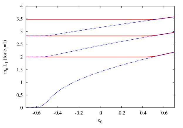
Figure 1: Masses of the first three massive modes in units of $L_{1}^{-1}$ as a function of $c_{0}$ for $L_{0}/L_{1}=10^{-15}$ and $c_{1}=1$. The solid (dotted) lines correspond to $[++]$ ($[-+]$) boundary conditions. Opposite boundary conditions are have identical masses with the replacement $c_{0,1}\to-c_{0,1}$.

The $z$-dependent Dirac mass shields the fermions from the deep IR. Of course, the heavier a particular KK mode is, the less it is shielded from the IR. This can be seen in Fig. 2, where we show the profiles of a LH zero mode and its first three massive KK modes for $[++]$ boundary conditions, with heavier modes propagating deeper in the IR. This has important phenomenological consequences. It has been shown that fields propagating sufficiently deep in the IR become eventually strongly coupled Karch:2006pv ; Falkowski:2008fz . This strong coupling does not affect the Standard Model (SM) fields, as they do not propagate deep enough in the IR (not even the top), but will signal the loss of perturbativity for heavy enough KK modes. In fact, we will see in the next section that, due to this effect, the contribution of fermionic KK modes to some EW observables decouples more slowly than one might naively expect.

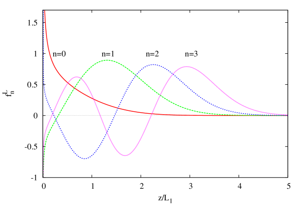
Figure 2: Left handed profiles of the zero mode and first three massive KK modes of a bulk fermion with $[++]$ boundary conditions, $c_{0}=0.4$ and $c_{1}=1$. Heavier KK modes propagate deeper in the IR.

The KK expansion of bulk fermions with a bulk Dirac mass of the form in Eq. (7) makes perfect sense independently of the Yukawa couplings to the bulk Higgs. Our goal in the rest of this article is to use this expansion to analyze the phenomenological implications of bulk fermions in soft wall models. We will do that by treating EWSB perturbatively, an approximation that will be carefully checked. This approach has the advantage that we can now trivially implement all the complications involved in fermion masses, from the generation of a large top mass to the generation of light fermion masses and their implication in flavor constraints of the model without having to resort to common bulk Dirac masses.

II.3 Fermion couplings

The KK expansion we have performed in the previous section allows us to compute the couplings we will need to investigate the EW and flavor implications of bulk fermions in the soft wall. One of the most relevant couplings is the Yukawa coupling between two fermions and a scalar. In the approximation we are considering, these couplings give the main contribution to SM fermion masses and mixings and also fix the mixings among fermion KK modes. These mixings in turn determine the fermion effects on EW precision observables and on flavor violating processes. Let us consider two bulk fermions $Q(x,z)$ and $T(x,z)$ coupled to a bulk scalar $\phi(x,z)$. We assume the scalar acquires a $z$ dependent vev $\langle\phi\rangle=f_{\phi}(z)v$, with $v$ a constant with dimension of mass and $f_{\phi}(z)$ normalized as

$$1=\int_{L_{0}}^{\infty}dz\,a^{3}e^{-\Phi}f_{\phi}^{2}(z).$$ (30)

When we identify the scalar with the Higgs responsible for EWSB, this normalization ensures that $v=174$ GeV, up to corrections of order $v^{2}L_{1}^{2}$. The part of the action involving the coupling between these three fields reads

$$S_{\mathrm{Yuk}} = \int d^{5}x\,\sqrt{g}e^{-\Phi}\Big{[}\lambda_{5}\bar{Q}\phi T+\mathrm{h.c.}\Big{]}=\int d^{5}x\,a\Big{[}\lambda_{5}\bar{q}\phi t+\mathrm{h.c.}\Big{]}=\int d^{5}x\,a\Big{[}\lambda_{5}vf_{\phi}\bar{q}t+\mathrm{h.c.}\Big{]}$$ (31)

$$= \int d^{4}x\,v\sum_{mn}\Bigg{\{}\lambda_{5}\left[\int dzaf_{\phi}f_{m}^{qL}f_{n}^{tR}\right]\bar{q}^{(m)}_{L}t_{R}^{(n)}+(L\leftrightarrow R)+\mathrm{h.c.}\Bigg{\}}$$

$$= \int d^{4}x\,v\sum_{mn}\Bigg{\{}\lambda_{mn}^{qt}\bar{q}^{(m)}_{L}t_{R}^{(n)}+\lambda_{mn}^{tq}\bar{t}^{(m)}_{L}q_{R}^{(n)}+\mathrm{h.c.}\Bigg{\}},$$

where $\lambda_{5}$ is a five-dimensional Yukawa coupling with mass dimensions $[\lambda_{5}]=-1/2$, naturally expected to be of order $\lambda_{5}\sim\sqrt{L_{0}}$. In the last equality we have defined the effective (dimensionless) four-dimensional Yukawa couplings between the different fermion KK modes. These are given by the five-dimensional Yukawa coupling times the overlap of the corresponding fermion KK modes with the scalar profile. Following the procedure in the KK expansion of fermions, we have defined $q(x,z)\equiv a^{2}e^{-\Phi/2}Q(x,z)$ and $t(x,z)\equiv a^{2}e^{-\Phi/2}T(x,z)$. Assuming a power-law scalar profile (see Appendix B)

$$f_{\phi}(z)=\frac{L_{1}}{L_{0}^{\frac{3}{2}}}\left[\frac{2}{\Gamma(\alpha-1,L_{0}^{2}/L_{1}^{2})}\right]^{\frac{1}{2}}\left(\frac{z}{L_{1}}\right)^{\alpha},$$ (32)

and identical localization for the LH and RH fermion zero modes ($c_{0,1}^{L}=-c_{0,1}^{R}$), we show the effective zero mode Yukawa coupling for different values of the Higgs profile in Fig. 3. The result is sensitive to the Higgs profile for $\alpha\lesssim 1.5$ but becomes essentially insensitive and very similar at the qualitative and quantitative level to the result in the hard wall for $\alpha\gtrsim 1.5$.

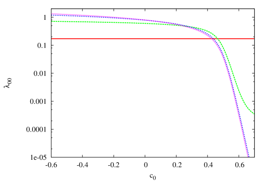
Figure 3: Effective four-dimensional Yukawa coupling for fermion zero modes with $\lambda_{5}=\sqrt{L_{0}}$ and $c_{1}^{L}=-c_{1}^{R}=1$ as a function of $c_{0}^{L}=-c_{0}^{R}\equiv c_{0}$ for different Higgs profiles. The different curves correspond, from bottom to top on the left hand side, to $\alpha=1,~{}1.33,~{}1.66,~{}2$. For $\alpha\gtrsim 1.5$ the zero mode spectrum is almost insensitive to the exact value of the Higgs profile.

The another very important coupling for the phenomenological implications of bulk fermions is the coupling of fermion and gauge boson KK modes. It comes from the gauge covariant derivative in the kinetic term of fermions and can be written as

$$S_{A\psi\psi} = \int d^{5}x\,g_{5}\bar{\psi}\cancel{A}\psi=\int d^{4}x\,\sum_{mnr}g_{5}\left[\int dzf_{m}^{L}f_{n}^{L}f_{r}^{A}\right]\bar{\psi}^{(m)}_{L}\cancel{A}_{r}\psi^{(n)}_{L}+(L\to R)$$ (33)

$$= \int d^{4}x\,\sum_{mnr}g_{4}^{{m_{L}}{n_{L}}r}\bar{\psi}^{(m)}_{L}\cancel{A}_{r}\psi^{(n)}_{L}+(L\to R),$$

where $g_{5}$ is the five-dimensional coupling constant, with mass dimension $[g_{5}]=-1/2$ and in the last equality we have defined the effective four-dimensional coupling between the fermionic modes $\psi_{L}^{(m)}$, $\psi_{L}^{(n)}$ and the $r$-th gauge boson KK mode. Of particular relevance is the coupling of fermion zero modes to gauge boson KK modes,

$$g_{n}(c_{0},c_{1})\equiv g_{4}^{{0}_{L}{0}_{L}n}=g_{5}\int dz\,(f_{0}^{L})^{2}f_{n}^{A},$$ (34)

which we show, in units of $g_{0}$ for the first three gauge boson KK modes, as a function of $c_{0}$ in Fig. 4 for $c_{1}=1$. The KK expansion of gauge bosons in our soft wall background is discussed in Appendix B. It is related to the fermionic expansion with the identification

$$f^{L}_{n}(c_{0}=1/2,c_{1}=1,z)=\sqrt{a}e^{-\Phi/2}f_{n}^{A}.$$ (35)

In particular we have

$$g_{n}(c_{0}=1/2,c_{1}=1)=g_{5}f_{0}^{A}\int dz\,ae^{-\Phi}f_{0}^{A}f_{n}^{A}=g_{0}\delta_{n0},$$ (36)

where we have used the fact the $f_{0}^{A}$ is $z$ independent, $g_{5}f_{0}^{A}=g_{0}$ and orthonormality of the gauge boson KK modes, see Eq. (91). Thus, for $c_{0}=1/2$ and $c_{1}=1$ the couplings to all the gauge boson KK modes vanish. Similarly, for $c_{0}\gtrsim 1/2$, the fermion zero modes are effectively localized towards the UV brane and their coupling to the gauge boson KK modes becomes independent of the exact localization (the value of $c_{0,1}$). For instance, the coupling to the first gauge boson KK mode becomes

$$g_{1}(c_{0}>\frac{1}{2}+\epsilon)\approx-\frac{g_{0}}{\sqrt{2\log\frac{L_{1}}{L_{0}}}}\approx-0.12g_{0},\quad\mbox{ (for $L_{0}/L_{1}\sim 10^{-15}$)}.$$ (37)

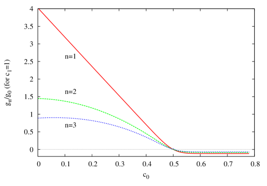
Figure 4: Coupling of a LH fermion zero mode to the first three gauge boson KK modes in units of the coupling to the gauge boson zero mode, as a function of $c_{0}$ for fixed $c_{1}=1$.

This universality of couplings for fermions localized towards the UV brane is the basis of the success of flavor physics in models with warped extra dimensions with a hard wall. The so called RS GIM mechanism in hard wall models stands for the fact that FCNC processes involving light quarks are suppressed by either light quark masses or by small CKM mixing angles. The origin of such suppression comes from the fact that the deviation from universality of the couplings to the gauge boson KK modes scale like the Yukawa couplings

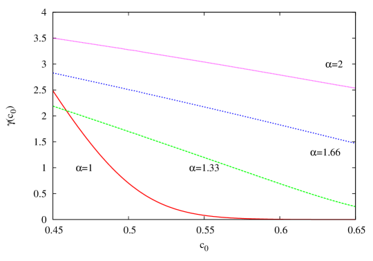
Figure 5: $\gamma(c_{0})^{\mathrm{soft}}$ as defined in Eq. (40). This quantity measures the scaling of the non-universality of couplings of light fermions to gauge boson KK modes with the masses of the light fermions. We have fixed $c_{1}^{q}=-c_{1}^{t}=c_{1}$, $c_{0}^{q}=c_{0}^{t}=c_{0}$, $\lambda_{5}=\sqrt{L_{0}}$ and shown different lines for different Higgs profiles.

$$\frac{g^{L,R}_{n}}{g_{0}}\approx\mathrm{const.}+f_{c_{L,R}}^{2}\gamma(c_{L,R}),$$ (38)

where $c_{L,R}$ is the localization parameter of the corresponding LH or RH fermion zero mode, $\gamma(c)$ is a slowly varying function of $c$, expected to be of order $\sqrt{\log L_{1}/L_{0}}\approx 5-6$ in the hard wall and $f_{c_{L,R}}$ determine the effective Yukawa couplings as

$$\lambda_{00}\sim f_{c_{L}}f_{c_{R}}.$$ (39)

To test how close to this property we are in our soft wall models, we computed the following quantity

$$\gamma(c_{0})^{\mathrm{soft}}\equiv\frac{[g_{n}(c_{0},c_{1})-g_{n}(c_{0}\to\infty,c_{1})]/g_{0}}{\lambda_{00}^{qt}(c_{0}^{q}=-c_{0}^{t}=c_{0},c_{1}^{q}=-c_{1}^{t}=c_{1})},$$ (40)

which is the equivalent of $\gamma(c)$ in the hard wall for identical localization of left and right components. The result for the coupling to the first gauge boson KK mode, for $c_{1}=1$ and $\lambda_{5}=\sqrt{L_{0}}$ is displayed in Fig. 5, for different values of the Higgs profile. It is obvious that for $\alpha\gtrsim 1.5$, for which we can obtain hierarchical fermion masses through wave function localization, similar scaling with the masses as the one that leads to a RS GIM protection occurs in the soft wall. Thus, one would expect that models with a soft wall behave in a very similar way as hard wall models do regarding flavor physics flavor ; Csaki:2009bb .

II.4 Validity of the approximation

The validity of the approximation we are employing in this work, namely a perturbative treatment of EWSB, has been recently subject to debate in hard wall models (see for instance Goertz:2008vr ; Csaki:2009bb ). In such models, it is clear that, if one was able to include the full tower of KK modes and diagonalized the infinite resulting mass matrix, the results should be equivalent to including EWSB effects exactly through the equations of motion. The rapid increase in KK masses also guarantees that in general, except in certain cases in which the induced off-diagonal masses are very large, the first few modes give a good enough approximation for the required level of precision. A perturbative treatment of EWSB is not useful only for soft wall models. In fact, even in hard wall models, there is only a few special cases, notably a brane localized Higgs and models of gauge-Higgs unification, in which EWSB effects can be included analytically. The validity of a perturbative treatment of EWSB is not so obvious in soft wall models, since the extra dimension extends to infinity and Higgs effects in the deep IR could modify the equations of motion in a way that cannot be reproduced with a finite number of modes computed in the absence of EWSB and a perturbative inclusion of the latter. This is in fact what happens in the case that the fermion Dirac mass is constant in the extra dimension so that the KK expansion in the absence of EWSB lacks a zero mode that should make up for most of the lightest mode in the full solution. With our assumption of fermion Dirac masses, however, the KK expansion in the absence of EWSB is well defined and all fields, including the zero modes are shielded from the deep IR. We can therefore expect, in general, EWSB effects to be a small perturbation and a finite number of KK modes to give a good enough approximation. Nevertheless, it is important to check the validity of the approximation at the quantitative level, especially in the case of the top quark, which is expected to suffer the strongest deviations. Even more so in soft wall models due to the fact we mentioned above that heavier KK modes propagate deeper in the IR and therefore get larger mass mixings.

We have checked the validity of the approximation both analytically and numerically. First, we have considered the case that can be solved analytically of common constant bulk Dirac masses and a quadratic Higgs profile. Let us consider again two bulk fermions $Q(x,z)$ and $T(x,z)$ but let us include the effect of the Yukawa coupling, Eq. (31) in the KK expansion. The equations of motion derived from the corresponding action read

$$i\cancel{\partial}\begin{pmatrix}q_{R,L}\\ t_{R,L}\end{pmatrix}\mp\partial_{5}\begin{pmatrix}q_{L,R}\\ t_{L,R}\end{pmatrix}-a\begin{pmatrix}M_{q}(z)&m(z)\\ m(z)&M_{t}(z)\end{pmatrix}\begin{pmatrix}q_{L,R}\\ t_{L,R}\end{pmatrix}=0,$$ (41)

where $M_{q,t}$ are our constant plus $z$ dependent mass for the bulk fermions (with parameters $c^{q,t}_{0,1}$) and $m(z)\equiv\lambda_{5}vf_{\phi}(z)$. Assuming a quadratic profile for the scalar and $c_{0}^{q}=c_{0}^{t}\equiv c_{0}$, the mass matrix reads

$$a\begin{pmatrix}M_{q}(z)&m(z)\\ m(z)&M_{t}(z)\end{pmatrix}=\frac{c_{0}}{z}\begin{pmatrix}1&0\\ 0&1\end{pmatrix}+\frac{z}{L_{1}^{2}}\begin{pmatrix}c_{1}^{q}&c_{m}\\ c_{m}&c_{1}^{t}\end{pmatrix}.$$ (42)

Let us now define the $2\times 2$ unitary matrix that diagonalizes the second term

$$U^{\dagger}\begin{pmatrix}c_{1}^{q}&c_{m}\\ c_{m}&c_{1}^{t}\end{pmatrix}U=\begin{pmatrix}c_{1}^{+}&0\\ 0&c_{1}^{-}\end{pmatrix}.$$ (43)

Then the equations of motion for the rotated fields

$$\begin{pmatrix}\psi^{+}\\ \psi^{-}\end{pmatrix}\equiv U^{\dagger}\begin{pmatrix}q\\ t\end{pmatrix},$$ (44)

are decoupled

$$i\cancel{\partial}\psi_{L,R}^{i}\pm\partial_{5}\psi_{R,L}^{i}-\left(\frac{c_{0}}{z}+\frac{c_{1}^{i}z}{L_{1}^{2}}\right)\psi_{R,L}^{i}=0,\quad i=+,-,$$ (45)

which can be solved analytically. One has to be careful that the boundary conditions mix both fields and therefore the physical modes live in the expansion of both of them

$$\psi_{L,R}^{i}=\sum_{n}f_{n}^{i\,L,R}\psi^{(n)}_{L,R},$$ (46)

where $\psi^{(n)}$ is independent of $i$. The orthonormality condition is then

$$\int_{L_{0}}^{\infty}dz\,\left[f_{n}^{+\,L}f_{m}^{+\,L}+f_{n}^{-\,L}f_{m}^{-\,L}\right]=\int_{L_{0}}^{\infty}dz\,\left[f_{n}^{+\,R}f_{m}^{+\,R}+f_{n}^{-\,R}f_{m}^{-\,R}\right]=\delta_{nm}.$$ (47)

We have compared the exact fermion masses and the couplings to gauge bosons with the ones we obtain using our perturbative treatment of EWSB. We have compared them for different values of $c_{0}$ and $c_{1}^{q,t}$, with $\lambda_{5}$ (equivalently $c_{m}$) fixed to reproduce the top mass for the lightest mode. The result of such comparison is that both the masses and the couplings agree to better than per mille level for values of $\lambda_{5}$ below the strong coupling limit, with the inclusion of just a few KK modes. Only when $\lambda_{5}$ is so large that the theory becomes non-perturbative close to the scale of the mass of the first KK mode the departure gets close to $\sim 10\%$.

We have been able to test the accuracy of our approximation in the case of common constant bulk Dirac masses. However, this is not the most general situation we will deal with in the study of the phenomenological implications of bulk fermions. We have also checked the case of different Dirac masses by numerically solving the set of coupled differential equations. Again the result for both masses and couplings is in excellent agreement with our approximation for perturbative values of $\lambda_{5}$.

III Electroweak Constraints on Soft Wall Models

As an application of our formalism, we investigate in this section the EW constraints on soft wall models. We consider a minimal realistic set-up with a custodially symmetric $SU(2)_{L}\times SU(2)_{R}\times U(1)_{X}$ bulk gauge symmetry broken to the SM gauge group $SU(2)_{L}\times U(1)_{Y}$ on the UV brane.

The bosonic action is given by

$$S_{b} = \int d^{5}x\,\sqrt{g}\,\mathrm{e}^{-\Phi}\Bigg{[}-\frac{1}{4}L_{MN}^{a}\,L^{a\,MN}-\frac{1}{4}R_{MN}^{a}\,R^{a\,MN}-\frac{1}{4}X_{MN}X^{MN}$$ (48)

$$\phantom{\int d^{5}x\,\sqrt{g}\,\mathrm{e}^{-\Phi}}+\mathrm{Tr}\,[(D_{M}H)^{\dagger}D^{M}H]-V(H)\Bigg{]}-\int d^{4}x\,\sqrt{-g_{UV}}{\rm e}^{-\Phi}\,V_{UV}(H)\,,$$

where $a=1,2,3$, $L^{a}_{M}$, $R_{M}^{a}$ and $X_{M}$ are the $SU(2)_{L}$, $SU(2)_{R}$ and $U(1)_{X}$ gauge fields, respectively, and $H$ is the bulk Higgs boson that transform as an $SU(2)_{L}\times SU(2)_{R}$ bidoublet

$$H(x,z)=\frac{1}{\sqrt{2}}\left(\begin{array}[]{cc}\phi_{0}^{*}(x,z)&\phi^{+}(x,z)\\ -\phi^{-}(x,z)&\phi_{0}(x,z)\end{array}\right)\,.$$ (49)

$V(H)$ and $V_{UV}(H)$ are the bulk and UV brane Higgs potentials. Choosing appropriately these potentials we can obtain a power-like profile for the Higgs vev (see Appendix B)

$$\langle H\rangle=\frac{f_{\phi}(z)}{\sqrt{2}}\begin{pmatrix}v&0\\ 0&v\end{pmatrix},$$ (50)

where $f_{\phi}(z)$ has been defined in Eq. (32) and, as we show below, $v=174$ GeV up to corrections of order $v^{2}L_{1}^{2}$. The UV boundary conditions satisfied by the gauge fields are

$$\partial_{5}L^{a}_{\mu}\big{|}_{L_{0}}=\partial_{5}B_{\mu}\big{|}_{L_{0}}=R_{\mu}^{1,2}\big{|}_{L_{0}}=Z_{\mu}^{\prime}\big{|}_{L_{0}}=0\,,$$ (51)

where we have defined

$$B_{\mu}=\frac{g_{X}R_{\mu}^{3}+g_{5}X_{\mu}}{\sqrt{g_{5}^{2}+g_{X}^{2}}},\quad Z_{\mu}^{\prime}=\frac{g_{5}R_{\mu}^{3}-g_{X}X_{\mu}}{\sqrt{g_{5}^{2}+g_{X}^{2}}},$$ (52)

with $B_{\mu}$ the hypercharge gauge boson, $g_{5}$ the gauge coupling of $SU(2)_{L}$ and $SU(2)_{R}$ which are taken equal to maintain the the $L\leftrightarrow R$ symmetry that protects the $Zb\bar{b}$ coupling Agashe:2006at and $g_{X}$ the $U(1)_{X}$ gauge coupling. The gauge couplings associated to $B_{\mu}$ and $Z_{\mu}^{\prime}$ are, respectively

$$g_{5}^{\prime}=\frac{g_{5}g_{X}}{\sqrt{g_{5}^{2}+g_{X}^{2}}},\quad g_{Z^{\prime}}=\sqrt{g_{5}^{2}+g_{X}^{2}},$$ (53)

whereas the associated charges are

$$Y=T^{3}_{R}+Q_{X},\quad Q_{Z^{\prime}}=\frac{g_{5}^{2}T^{3}_{R}-g_{X}^{2}Q_{X}}{g_{5}^{2}+g_{X}^{2}}.$$ (54)

III.1 Bosonic contribution to electroweak precision observables

In this section we review the bosonic contribution to EW precision observables in soft wall models Falkowski:2008fz ; Batell:2008me . If the light SM fermions are localized towards the UV brane, models with warped extra dimension, including soft wall models, fall in the class of universal new physics models Barbieri:2004qk . In that case, all relevant constraints can be obtained in terms of four oblique parameters, which are computed from the quadratic terms in the effective Lagrangian of the interpolating fields that couple universally to the SM fermions. The holographic method Barbieri:2003pr gives the most straight-forward calculation of the oblique parameters as it gives directly the effective Lagrangian for the interpolating fields. In the spirit of the approximations we have used with fermions, we will include EWSB effects perturbatively, which allows us to consider arbitrary Higgs profiles. The leading order in the expansion in the EWSB scale $v$ does not give the correction to the $T$ parameter (which requires $v^{4}$ terms) but we nevertheless know that the tree level contribution to the $T$ parameter vanishes due to the custodial symmetry. The leading correction to all other three oblique parameters can be safely computed perturbatively.

The procedure can be performed as follows. First we set to zero the fields that are not sourced on the UV brane, leaving only the SM gauge bosons. The relevant part of the action reads

$$S=\int d^{5}x\sqrt{g}\mathrm{e}^{-\Phi}\left\{-\frac{1}{4g_{5}^{2}}L_{MN}^{a}L^{a\,MN}-\frac{1}{4g_{5}^{\prime\,2}}B_{MN}B^{MN}+\frac{v^{2}f_{\phi}^{2}}{4}\Big{[}(L^{b}_{M})^{2}+(L^{3}_{M}-B_{M})^{2}\Big{]}\right\},$$ (55)

where in this section, we are using non-canonically normalized fields. The term in square brackets is the mass term due to EWSB, that we will treat as a perturbation.  Going to 4D momentum space, and considering the $\mu$ components of the gauge fields, we define

$$L^{a}_{\mu}(p,z)=f(p,z)\bar{L}^{a}_{\mu}(p),\quad B_{\mu}(p,z)=f(p,z)\bar{B}_{\mu}(p),$$ (56)

with $f(p,z)$ fixed by the bulk equations of motion, which are identical for $L^{a}$ and $B$. With the boundary condition $f(p,L_{0})=1$,

$$f(p,z)=U\left(-\frac{p^{2}L_{1}^{2}}{4},0,\frac{z^{2}}{L_{1}^{2}}\right)\Big{/}U\left(-\frac{p^{2}L_{1}^{2}}{4},0,\frac{L_{0}^{2}}{L_{1}^{2}}\right).$$ (57)

Integrating out the bulk we obtain an effective action for the 4D interpolating fields

$$S_{\mathrm{hol.}}=-\frac{1}{2}\int\frac{d^{4}p}{(2\pi)^{4}}\eta^{\mu\nu}\left\{\bar{L}^{b}_{\mu}\Pi_{+-}(p^{2})\bar{L}^{b}_{\nu}+\bar{L}^{3}_{\mu}\Pi_{33}(p^{2})\bar{L}^{3}_{\nu}+\bar{B}_{\mu}\Pi_{BB}(p^{2})\bar{B}_{\nu}+2\bar{L}^{3}_{\mu}\Pi_{3B}\bar{B}_{\nu}\right\}+\ldots$$ (58)

where the different form factors read

$$\Pi_{+-}(p^{2}) = \Pi_{33}(p^{2})=\frac{1}{g_{5}^{2}}\Pi_{0}(p^{2})-\Pi_{\phi}(p^{2}),$$ (59)

$$\Pi_{BB}(p^{2}) = \frac{1}{g_{5}^{\prime\,2}}\Pi_{0}(p^{2})-\Pi_{\phi}(p^{2}),$$ (60)

$$\Pi_{3B}(p^{2}) = \Pi_{\phi}(p^{2})\,,$$ (61)

with the EW symmetry preserving term

$$\Pi_{0}(p^{2})\equiv e^{-\Phi}\partial_{5}f(p,z)\Big{|}_{z={L_{0}}}\approx p^{2}L_{0}\left(\log\frac{L_{1}}{L_{0}}-\frac{\gamma_{E}}{2}\right)+\frac{p^{4}}{2}L_{0}\frac{\pi^{2}L_{1}^{2}}{24}+\ldots,$$ (62)

where $\gamma_{E}\approx 0.577$ is the Euler-Mascheroni constant. In the second expression we have expanded in powers of $p^{2}$ and assumed $L_{0}/L_{1}\ll 1$. The EWSB term is

$$\Pi_{\phi}(p^{2})=\frac{v^{2}}{2}\int dz\,a^{3}e^{-\Phi}f_{\phi}^{2}f^{2}(p,z)=\frac{v^{2}}{2}+\mathcal{O}(p^{2}).$$ (63)

The gauge couplings and the EWSB scale are fixed by the following conditions

$$\Pi_{+-}^{\prime}(0)=\frac{1}{g^{2}},\quad\Pi_{BB}^{\prime}(0)=\frac{1}{g^{\prime\,2}},\quad\Pi_{+-}(0)=-\frac{(174~{}\mathrm{GeV})^{2}}{2},$$ (64)

where a prime here denotes derivative with respect to $p^{2}$. They imply, up to corrections $\mathcal{O}(v^{2}L_{1}^{2})$,

$$\frac{g_{5}}{g}=\frac{g_{5}^{\prime}}{g^{\prime}}=\sqrt{L_{0}\left(\log\frac{L_{1}}{L_{0}}-\frac{\gamma_{E}}{2}\right)},$$ (65)

and

$$v=174~{}\mathrm{GeV}.$$ (66)

The oblique parameters are defined in terms of these form factors. Recall that the first equality in Eq. (59) does not give the leading correction to the $T$ parameter, which appears at order $v^{4}$ in the form factors. The other three relevant oblique parameters are defined by

$$S = 16\pi\Pi^{\prime}_{3B}(0)=-16\pi g^{2}\Pi_{\phi}^{\prime}(0),$$ (67)

$$W = \frac{g^{2}m_{W}^{2}}{2}\Pi_{33}^{\prime\prime}(0),$$ (68)

$$Y = \frac{g^{\prime\,2}m_{W}^{2}}{2}\Pi_{BB}^{\prime\prime}(0).$$ (69)

Inserting the corresponding coefficients we obtain, for $W$ and $Y$,

$$W=Y=\frac{g^{2}\pi^{2}}{96\left(\log\frac{L_{1}}{L_{0}}-\frac{\gamma_{E}}{2}\right)}(vL_{1})^{2}+\ldots$$ (70)

which is volume ($\log(L_{1}/L_{0})-\gamma_{E}/2$) suppressed and therefore leads to a very mild constraint on $L_{1}$.

Figure 6: $L_{1}^{-1}$ as a function of the Higgs localization parameter $\alpha$ such that $S=0.2$ using Eq. (67).

The $S$ parameter on the other hand can in general only be computed numerically, except for particular values of the Higgs localization parameter $\alpha$. In general it is not volume suppressed so it gives a stronger constraint that $W$ and $Y$. This is easy to understand in an alternative derivation in which one integrates out the physical heavy KK modes to obtain an effective Lagrangian that is not oblique but has corrections to the gauge boson masses, which are volume enhanced, to vertex fermion-gauge couplings, which are order one, and to four-fermion interactions, which are volume suppressed. If one then introduces field redefinitions so that an oblique Lagrangian is obtained, all three types of corrections affect the $T$ parameter (which would be the leading constraint if it were not for the custodial symmetry that makes the total contribution to cancel). Only vertex corrections and four-fermion interactions enter in the $S$ parameter, which is therefore not expected to have any volume enhancement or suppression. Finally only the four-fermion interactions enter $W$ and $Y$, which explains why they are volume suppressed and therefore less constraining in general. We have computed the $S$ parameter as a function of the Higgs localization parameter $\alpha$. In Fig. 6 we show, as an example, the value of $L_{1}^{-1}$ that will result in a value $S=0.2$ as a function of $\alpha$. We have checked that our numerical result agrees exactly with the analytic results given in Batell:2008me for the cases $\alpha=1$ and $\alpha=2$ to leading order in $v^{2}L_{1}^{2}$. For $\alpha=1$, the Higgs profile times the metric is flat in the extra dimension and no vertex corrections are generated. Thus, the $S$ parameter only receives the volume suppressed contribution from four-fermion interactions, which results in a very mild constraint.

III.2 Fermionic contributions to electroweak observables

Our calculation in the previous section showed that the bosonic sector is less constrained by EW precision tests in soft wall models than in hard wall models. The large top mass however makes it reasonable that fermionic contributions to EW precision observables, most notably the $T$ parameter and the $Zb\bar{b}$ coupling, which have been neglected so far can be relevant. In fact, they are needed for light KK modes to be allowed, as the zero value of the tree level $T$ parameter is not compatible with a relatively large value of $S$.

We consider a minimal fermionic content compatible with the custodial and $LR$ symmetry that protect the $T$ parameter and $Zb\bar{b}$ coupling, respectively. Ignoring the bottom or lighter quark masses, the relevant fermionic sector consists of an $SU(2)_{L}\times SU(2)_{R}$ bidoublet $\psi_{(2,2)}=(X,Q)$ and an $SU(2)_{L}\times SU(2)_{R}$ singlet $T$, both with $Q_{X}=2/3$,

$$\psi_{(2,2)}=\left(\begin{array}[]{cc}X^{u}[-+]&Q^{u}[++]\\ X^{d}[-+]&Q^{d}[++]\end{array}\right)_{\frac{2}{3}},\quad T[--]_{2/3}\,,$$ (71)

where the subscript denotes the $U(1)_{X}$ charge and we have written explicitly the boundary conditions in soft-wall notation so that the second sign corresponds to the sign of the corresponding $c_{1}$. From the SM point of view $X$ and $Q$ are $SU(2)_{L}$ doublets with hypercharges $7/6$ and $1/6$ and they have $T^{3}_{R}=1/2$ and $-1/2$, respectively. The bc are chosen such that $Q$ has a left handed and $T$ has a right handed zero mode which correspond to the SM top sector $q_{L}$ and $t_{R}$. $X$ have no zero modes but have the IR bc fixed by the bulk gauge symmetry.

The couplings of the fermions to the gauge fields and the Yukawa couplings are given in Eq. (33) and Eq. (31). The latter are given in terms of the fermion profiles by

$$S_{\mathrm{Yuk}}=\int d^{4}x\,v\sum_{mn}\left\{\big{[}\lambda^{qt}_{mn}\bar{q}^{u\,(m)}_{L}+\lambda^{xt}_{mn}\bar{x}^{d\,(m)}_{L}\big{]}t^{(n)}_{R}+\bar{t}^{(m)}_{L}\big{[}\lambda^{tq}_{mn}q^{u\,(n)}_{R}+\lambda^{tx}_{mn}x^{d\,(n)}_{R}\big{]}+\mathrm{h.c.}\right\}.$$ (72)

These terms, together with the gauge couplings and KK masses allow us to compute the physical masses and physical couplings to the EW gauge and would-be Goldstone bosons. These are the required ingredients to compute the one loop fermionic contribution to the $T$ parameter and the $Zb\bar{b}$ coupling. We use the calculation of these two observables presented in Anastasiou:2009rv , which extended previous calculations Lavoura:1992np to a general enough set-up able to accommodate our fermionic spectrum.

We have investigated the dependence of the $T$ parameter and $Zb\bar{b}$ coupling as a function of our input parameters, $c_{0,1}^{q,t}$, with $\lambda_{5}$ adjusted so that the physical top mass is $m_{t}=172$ GeV. Before discussing the results, we should make two important comments. First, we are using as an example a very minimal fermionic spectrum, with no particularly light fermion KK modes. This is enough to prove that models of EWSB with a soft wall are compatible with EW precision tests for relatively light KK gauge boson modes. However, one could expect a richer behavior, similar to the one observed in hard wall models, if a more complicated fermionic spectrum, including twisted bc and bulk mixing terms is considered. Second, we have mentioned above that heavy KK modes propagate deeper in the IR and therefore they couple more strongly to the Higgs. This results in a slower decoupling of heavy modes regarding their contribution to the $T$ parameter (the $Zb\bar{b}$ coupling is less sensitive to this effect). In fact, we have observed that the $T$ parameter is quite unstable against the addition of new fermion KK modes for the first few modes and it stabilizes into a fixed value only after the inclusion of a relatively large $\sim 10$ number of KK levels. Note that, because of the scaling $m_{n}\sim\sqrt{n}$, the addition of many modes does not mean that we have to go to very high scales before the $T$ parameter is stable. This effect worsens the more towards the IR the Higgs is localized (i.e. the larger $\alpha$ is). For values $\alpha\gtrsim 2$, the number of modes required to stabilize the $T$ parameter gets close to the limit of strong coupling and it is difficult to make precise quantitative predictions. Thus, we will show most of our results for $\alpha=1.5$, although we have checked that these results do not change qualitatively when $\alpha$ gets closer to $2$.

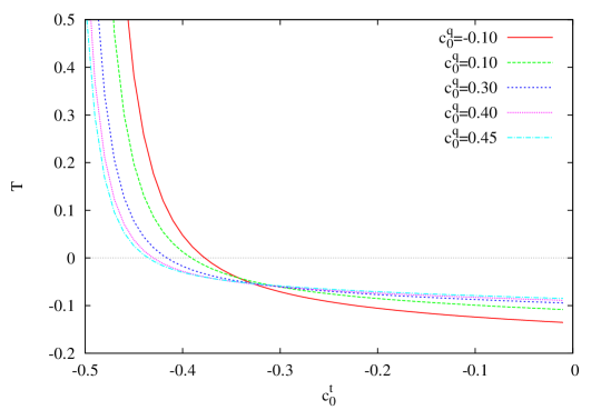
Figure 7: $T$ as a function of $c_{0}^{t}$ for different values of $c_{0}^{q}$ with fixed $1/L_{1}=1.2$ TeV, $c_{1}^{q}=1.2$, $c_{1}^{t}=-1$ and $\alpha=1.5$.

The results we have obtained for the $T$ parameter and the $Zb\bar{b}$ coupling can be summarized as follows.

• The $T$ parameter is negative in a large portion of parameter space, as was already observed in hard-wall models with the same fermionic quantum numbers Carena:2006bn . It is negative, with a very mild dependence on $c_{0}^{q,t}$ for values $c_{0}^{t}\gtrsim-0.35$, whereas it develops a strong dependence on the two parameters $c_{0}^{q,t}$ for values of $c_{0}^{t}\gtrsim 0.35$ becoming quickly positive and of order one. This behavior can be clearly seen in Fig. 7 where we plot the $T$ parameter as a function of $c_{0}^{t}$ for different values of $c_{0}^{q}$. The behavior shown extends to positive values of $c_{0}^{t}$ without any significant change.

• The $Zb\bar{b}$ coupling is much less sensitive to the different localization parameters, $c_{0,1}^{q,t}$. In fact, it is not even very sensitive to the particular value of $L_{1}$ (provided it is of $\sim$ TeV^-1 size) for a fixed value of the Higgs profile. The reason is that, increasing $L_{1}^{-1}$, which makes the KK modes more massive and therefore should decouple them, also makes the Higgs more IR localized, which increases the required value of $\lambda_{5}$ and the coupling among the heavy KK modes in such a way that both effects almost cancel each other giving rise to an essentially constant value of the $Zb\bar{b}$ coupling $\delta g_{b_{L}}\approx-(1-1.5)\times 10^{-3}$. This effect is in principle also present in the $T$ parameter but it is overcome by the larger number of heavy modes that contribute in that case and the strong dependence on $c_{0}^{q,t}$.

III.3 Fit to electroweak observables

Our analysis of the contribution to EW precision observables from the fermionic sector showed two main features for the class of models we have considered: the $Zb\bar{b}$ coupling receives a non-negligible, almost constant correction $\delta g_{b_{L}}\approx-(1-1.5)\times 10^{-3}$, and the $T$ parameter can get essentially any value for $c_{0}^{t}\lesssim-0.35$. Using these features we have performed a three parameter fit to all relevant electroweak precision observables, using an updated version of the code in Han:2004az (see Anastasiou:2009rv for details on the fit). The result is summarized in Fig. 8 in which we show the minimum value of the $\Delta\chi^{2}$ obtained in our model as a function of $L_{1}^{-1}$ for different values of the Higgs profile. The $\Delta\chi^{2}$ is defined as the $\chi^{2}$ for an arbitrary point of our model with the minimum $\chi^{2}$ optimizing the values of $T$, $S$ and $Zb\bar{b}$ coupling subtracted. In the figure we also show the values of $\Delta\chi^{2}$ that correspond to $95\%$ and $99\%$ C.L. limits for a fit to three variables.

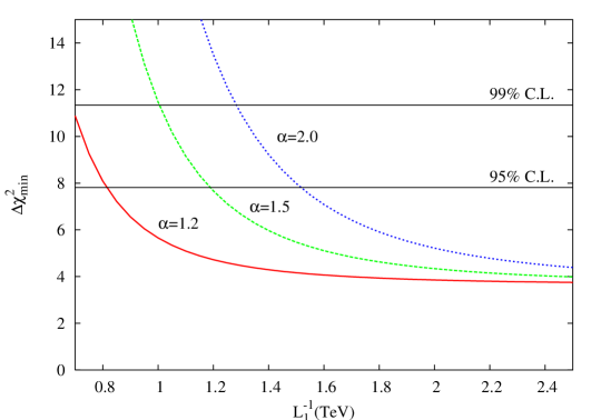
Figure 8: Minimum value of $\Delta\chi^{2}$ as described in the text as a function of $L_{1}^{-1}$ (in TeV) for different values of the Higgs profile. The horizontal lines show the $95\%$ and $99\%$ C.L. limits on the $\Delta\chi^{2}$ for a fit with three variables.

The corresponding bounds on $L_{1}^{-1}$ read, at $95\%$ C.L.

$$L_{1}^{-1}\mbox{ (in TeV)}\lesssim 0.85,~{}1.2,~{}1.55\mbox{ for }\alpha=1.2~{},1.5~{}2,$$ (73)

which translate into the following values for the gauge boson KK modes

$$m^{\mathrm{GB}}_{n}\sim\left\{\begin{array}[]{ll}1.7,~{}2.4,~{}3,\ldots&(\alpha=1.2),\\ 2.4,~{}3.4,~{}4.2,\ldots&(\alpha=1.5),\\ 3.1,~{}4.4,~{}5.4,\ldots&(\alpha=2).\end{array}\right.$$ (74)

Note that, even for $\alpha$ close to one, the bound is more stringent than one would naively get from the $S$ parameter alone. The main reason is the almost constant contribution to the $Zb\bar{b}$ coupling that creates some tension in the fit. Of course, a richer fermionic spectrum than we have considered in our minimal model could result in a different value of this coupling and therefore a smaller bound.

IV Discussion

Models with warped extra dimensions and a soft IR wall represent a more general approach to EWSB than hard wall models. The spectrum of KK excitations is sensitive to the details of the soft wall and an analysis of the bosonic sector, assuming the SM fermions to be localized at the UV brane, shows that current EW constraints are compatible with very light $\sim$ TeV new resonances. UV localized fermions are a good approximation regarding the implications on EW observables of the light fermions. However, flavor constraints and top dependent contributions to EW observables cannot be studied in that approximation. We have developed the tools to analyze bulk fermions in soft wall models with great generality. By assuming a position dependent Dirac mass for the bulk fermions, which could be generated by a direct coupling to the soft wall, we can perform the KK expansion of bulk fermions in a very general set-up. Our construction reproduces well the most relevant features of bulk fermions present in hard wall models, like the effect of non-trivial IR boundary conditions, the presence of ultra-light modes for twisted boundary conditions, flavor universality of couplings of UV localized fermions to KK gauge bosons or hierarchical Yukawa couplings through wave function localization. Using these techniques we have studied the flavor structure of realistic models with the result that a similar flavor protection as the one observed in hard wall models can be expected. Similarly, we have computed the contribution of the top sector to EW precision observables and shown that simple realistic models with custodial symmetry and KK excitations as light as

$$m_{1}\gtrsim 1.7~{}\mbox{TeV},$$ (75)

can be compatible with all EW precision tests. Furthermore, the particular realization of the soft wall we have considered predicts a linear scaling of the mass squared of the KK excitations. As an example, for certain Higgs profile ($\alpha=1.5$) we can have, at the $95\%$ C.L., the following spectrum of new gauge boson KK masses

$$m_{n}\approx 2\sqrt{n}\times 1.2~{}\mbox{TeV}\approx(2.4,~{}3.2,~{}4.2)~{}\mbox{TeV}.$$ (76)

Detailed analyses in hard wall models showed that masses $m_{KK}^{\mathrm{G}}\lesssim 4-5$ TeV in the case of KK gluons Agashe:2006hk and $m_{KK}^{\mathrm{EW}}\lesssim 2$ TeV in the case of KK excitations of the EW bosons Agashe:2007ki could be reached at the LHC with $\sim 100-300~{}\mathrm{fb}^{-1}$. It would therefore seem that the first and maybe even the second mode of KK gluons could be observable at the LHC although a detailed analysis, taking into account the details of the spectrum in our model, is required to fully assess the LHC reach.

Regarding the fermionic sector, we have chosen a very minimal set-up, with just the minimal number of five-dimensional fields to reproduce the observed spectrum. In that case no particularly light KK fermions are present in the spectrum. Due to the boundary conditions, the KK excitations of $X$, which from the SM point of view is an $SU(2)_{L}$ doublet of hypercharge $7/6$ are among the lightest new fermions with a mass $m_{1}^{X}\sim 2-2.5$ TeV. This multiplet includes a charge $5/3$ quark that was shown to be easily reachable in an early LHC run through pair production provided it is light enough Contino:2008hi . The analysis in that reference only considered $0.5$ and $1$ TeV masses. Most likely, masses as heavy as the ones we obtain are not reachable at the LHC through pair production. Single production is a more likely possibility but again a detailed analysis would be required to understand the real reach. This simple fermionic spectrum was chosen for simplicity. It is not a constraint coming from the soft wall. Richer structures are easy to implement. For instance, one could simulate the spectrum used in hard wall realistic models of gauge-Higgs unification Carena:2006bn ; Panico:2008bx by introducing further bulk fermions with twisted boundary conditions and a position dependent mass term mixing them. In that case we can only solve analytically for a common $z$-independent mass, which is still tolerable for the top quark. This richer fermionic spectrum would lead to lighter quarks associated to the top and could make new regions in parameter space compatible with EW precision data through their contribution to EW precision observables. Bulk fermions can be also implemented in actual composite Higgs models in the soft wall Falkowski:2008fz using the techniques developed in this work.

Our results show that soft wall models have the potential to become realistic models of EWSB readily accessible at the LHC. We have gone a step forward towards this goal by including with great generality bulk fermions in these models. However, several further steps need to be taken before we can consider these models a full satisfactory solution to the hierarchy problem. One of the most pressing open questions is that of the stability of the soft wall and the corresponding $L_{1}/L_{0}\sim\mathrm{TeV}/M_{\mathrm{Pl}}$ hierarchy. Also, given the new bounds and the different patterns of masses and mixings that can be obtained in soft wall models, a new analysis of the LHC reach would be welcome. Finally, soft wall models open the possibility to study a priori completely different physics, like unparticles, and their relation to EWSB. It has been recently shown that the Higgs itself could be part of the conformal sector (Unhiggs). It can be modeled by a continuum of resonances in a 5D soft wall model Stancato:2008mp ; Falkowski:2008yr , being (partly) responsible for EWSB and longitudinal gauge boson scattering and even being able to reproduce the quantum contributions of a standard Higgs to the oblique parameters despite having modified (suppressed) couplings to the SM fields. It would be very interesting to use the formalism we have developed here to analyze the effect of the top quark propagating in such background.

Appendix A Background solution

The soft wall model that we have considered in this article can be obtained dynamically from a five dimensional gravitational model Batell:2008zm ; Batell:2008me . We collect the relevant results in this appendix. More details can be found in the original references. The action describes gravity coupled to two scalars, the dilaton $\Phi$ and the tachyon $T$,

$$S = \int d^{5}x\sqrt{g}\,\Bigg{[}M^{3}R-\frac{1}{2}g^{MN}\partial_{M}\Phi\partial_{N}\Phi-\frac{1}{2}g^{MN}\partial_{M}T\partial_{N}T-V(\Phi,T)\Bigg{]}$$ (77)

$$\hskip 56.9055pt-\int d^{4}x\sqrt{-g_{UV}}\lambda_{UV}(\Phi,T)\,,$$

where $M$ is the $5$D Planck mass and $V(\Phi,T)$ and $\lambda_{UV}(\Phi,T)$ are the scalar bulk and UV boundary potentials for the dilaton and the tachyon and are given by

$$V(\Phi,T) = 18\Bigg{[}\left(\frac{\partial W}{\partial\Phi}\right)+\left(\frac{\partial W}{\partial T}\right)\Bigg{]}-\frac{12}{M^{3}}W^{2}\,,$$

$$\lambda_{UV}(\Phi,T) = 6\Bigg{[}W(\Phi_{0},T_{0})+\partial_{\Phi}W(\Phi_{0},T_{0})(\Phi-\Phi_{0})+\partial_{T}W(\Phi_{0},T_{0})(T-T_{0})+\dots\Bigg{]}\,,$$ (78)

where $W$ is

$$W(\Phi,T)=\frac{M^{3}}{L_{0}}\Bigg{[}(\nu-1){\rm e}^{T^{2}/(24(1+1/\nu)M^{3})}-\nu\left(1-\frac{\Phi}{\sqrt{6}M^{3/2}}\right){\rm e}^{\Phi/(\sqrt{6}M^{3/2})}\Bigg{]}\,.$$ (79)

Solutions for the equations of motions for the dilaton and the tachyon using the above potentials can be found as

$$\Phi(z) = \sqrt{\frac{8}{3}}M^{3/2}\left(\frac{z}{L_{1}}\right)^{\nu}\,,$$

$$T(z) = \pm 4\sqrt{1+1/\nu}M^{3/2}\left(\frac{z}{L_{1}}\right)^{\nu/2}\,,$$ (80)

where the background metric is chosen to be

$$g_{MN}=a^{2}(z)\,{\rm e}^{-4/3(z/L_{1})^{\nu}}\,\eta_{MN}.$$ (81)

Note that one can recover the metric in Eq. (1) and the action in Eq. (2) by the redefinitions

$$\Phi \rightarrow \sqrt{\frac{3}{8}}M^{-3/2}\Phi\,$$

$$g_{MN} \rightarrow {\rm e}^{4/3(z/L_{1})^{\nu}}g_{MN}\,.$$ (82)

Throughout this paper, we considered the case with $\nu=2$ only.

Appendix B Bulk Bosonic Fields in the Soft Wall

In this Appendix we review the Kaluza-Klein expansion of bulk bosonic fields in the soft wall. Further details can be found in Batell:2008me .

B.1 Bulk Higgs

Let us assume the following form for the bulk and the UV boundary Higgs potentials $V(H)$ and $V_{UV}(H)$ in Eq. (48)

$$V(H) = m_{H}^{2}(z)\,{\rm Tr}\,|H|^{2}\,,$$

$$V_{UV}(H) = \lambda_{0}\,L_{0}^{2}\left({\rm Tr}\,|H|^{2}-v_{0}^{2}\right)^{2}\,,$$ (83)

where the effective mass for the bulk Higgs is defined to have the form

$$m_{H}(z)^{2}=\frac{1}{L_{0}^{2}}\left[\alpha(\alpha-4)-2\alpha\frac{z^{2}}{L_{1}^{2}}\right]\,.$$ (84)

The above mass term is assumed to arise from a coupling to another scalar which gets a background vev. The UV boundary potential is added to the action in Eq. (48) so that the solutions of the equations of motion for the Higgs field satisfy non-trivially the UV boundary conditions. Solving for the equation of motion for the bulk Higgs using $V(H)$ and demanding that the solution is finite in the soft wall background, one finds

$$f_{h}(z)=c_{h}\,z^{\alpha}\,,$$ (85)

where $c_{h}$ is a normalization constant and we have defined the Higgs vev as

$$\langle H\rangle=\frac{f_{h}(z)}{\sqrt{2}}\begin{pmatrix}v&0\\ 0&v\end{pmatrix},$$ (86)

with $v$ a constant with mass dimension 1. The UV boundary condition satisfied by the above solution is given in Ref. Batell:2008me . Properly normalizing the bulk Higgs field and solving for the mass of the $W$ boson in terms of the overlaps of the bulk Higgs profile with the gauge field zero modes for the $W$ we find that

$$c_{h}=\sqrt{\frac{2L_{1}^{2}}{L_{0}^{3}}}\frac{1}{\sqrt{\Gamma(\alpha-1,L_{0}^{2}/L_{1}^{2})}}\,$$ (87)

with $\Gamma$ the incomplete Gamma function, and $v=174$ GeV, up to corrections $\mathcal{O}(v^{2}L_{1}^{2})$. It was shown in Batell:2008me that this solution is indeed the ground state of the theory.

B.2 Gauge bosons

The expansion of gauge bosons in our background was also considered in Batell:2008me and we collect here the main results. The action for a bulk $U(1)$ gauge field reads

$$S=-\frac{1}{4}\,\int d^{5}x\,\sqrt{g}{\rm e}^{-\Phi}\,A_{MN}A^{MN}\,.$$ (88)

We perform the standard KK decomposition

$$A_{\mu}(x,z)=\sum_{n}f_{n}^{A}(z)A_{\mu}^{(n)}(x),$$ (89)

where the four dimensional fields $A_{\mu}^{(n)}(x)$ satisfy the four dimensional equations of motion for a gauge massive gauge boson with mass $m_{n}$. The profile functions $f_{n}^{A}(z)$ satisfy then the following equation

$$\Big{[}\partial_{5}^{2}+\left(\frac{a^{\prime}}{a}-\Phi^{\prime}\right)\partial_{5}+m_{n}^{2}\Big{]}f_{n}^{A}=0,$$ (90)

and normalization condition

$$\int_{L_{0}}^{\infty}dz\,ae^{-\Phi}f_{m}^{A}f_{n}^{A}=\delta_{mn}.$$ (91)

Applying the change of variable

$$x=\frac{z^{2}}{L_{1}^{2}}\,,$$ (92)

and inserting the explicit form of the metric and the dilaton field, the equation for the bosonic profile reads

$$\Bigg{[}x\partial^{2}_{x}-x\partial_{x}+\frac{L_{1}^{2}\,m_{n}^{2}}{4}\Bigg{]}f_{A}^{n}(z)=0\,,$$ (93)

which is the same equation $g(z)$ of Eq. (16) satisfied with the special values of fermionic parameters $c_{0}=1/2$ and $c_{1}=1$. The normalizable solution is given in terms of confluent hypergeometric function

$$f_{n}^{A}(z)=N_{n}^{A}\,U\left(\frac{-m_{n}^{2}\,L_{1}^{2}}{4},0,\frac{z^{2}}{L_{1}^{2}}\right)\,,$$ (94)

where the normalization constants $N_{n}^{A}$ are determined from Eq. (91). The masses for the massive gauge bosons are found by applying the corresponding boundary conditions. Applying Neumann boundary conditions for the UV brane one finds that the masses for the heavy modes are given approximately by

$$m_{n}^{2}\sim\frac{4}{L_{1}^{2}}\,n^{2}\,.$$ (95)

$U(0,0,z^{2})=1$ so the profile for a massless gauge boson zero mode is given entirely by its normalization constant,

$$f_{A}^{0}(z)=\sqrt{\frac{2}{L_{0}\,E_{1}(L_{0}^{2}/L_{1}^{2})}}\,,$$ (96)

where $E_{\nu}(z)=\int_{1}^{\infty}dt\,e^{-zt}/t^{\nu}$ is the Exponential Integral E function.

References

- (1) L. Randall and R. Sundrum, Phys. Rev. Lett. 83 (1999) 4690 [hep-th/9906064]; Phys. Rev. Lett. 83 (1999) 3370 [hep-ph/9905221].
- (2) J. M. Maldacena, Adv. Theor. Math. Phys. 2 (1998) 231 [Int. J. Theor. Phys. 38 (1999) 1113] [hep-th/9711200]; S. S. Gubser, I. R. Klebanov and A. M. Polyakov, Phys. Lett. B 428 (1998) 105 [hep-th/9802109]; E. Witten, Adv. Theor. Math. Phys. 2 (1998) 253 [hep-th/9802150].
- (3) N. Arkani-Hamed, M. Porrati and L. Randall, JHEP 0108 (2001) 017 [hep-th/0012148]; R. Rattazzi and A. Zaffaroni, JHEP 0104 (2001) 021 [hep-th/0012248]; M. Perez-Victoria, JHEP 0105 (2001) 064 [hep-th/0105048].
- (4) M. S. Carena, E. Ponton, J. Santiago and C. E. M. Wagner, Nucl. Phys. B 759 (2006) 202 [hep-ph/0607106]; Phys. Rev. D 76 (2007) 035006 [hep-ph/0701055]. R. Contino, L. Da Rold and A. Pomarol, Phys. Rev. D 75 (2007) 055014 [hep-ph/0612048].
- (5) G. Cacciapaglia, C. Csaki, G. Marandella and J. Terning, Phys. Rev. D 75 (2007) 015003 [hep-ph/0607146].
- (6) K. Agashe, A. Delgado, M. J. May and R. Sundrum, JHEP 0308 (2003) 050 [hep-ph/0308036].
- (7) K. Agashe, R. Contino, L. Da Rold and A. Pomarol, Phys. Lett. B 641 (2006) 62 [hep-ph/0605341].
- (8) H. Davoudiasl, J. L. Hewett and T. G. Rizzo, Phys. Rev. D 68 (2003) 045002 [hep-ph/0212279]; M. S. Carena, A. Delgado, E. Ponton, T. M. P. Tait and C. E. M. Wagner, Phys. Rev. D 68 (2003) 035010 [hep-ph/0305188]; Phys. Rev. D 71 (2005) 015010 [hep-ph/0410344]; A. Djouadi, G. Moreau and F. Richard, Nucl. Phys. B 773 (2007) 43 [hep-ph/0610173]; C. Bouchart and G. Moreau, Nucl. Phys. B 810 (2009) 66 [0807.4461 [hep-ph]].
- (9) A. Karch, E. Katz, D. T. Son and M. A. Stephanov, Phys. Rev. D 74 (2006) 015005 [hep-ph/0602229].
- (10) A. Falkowski and M. Perez-Victoria, JHEP 0812 (2008) 107 [0806.1737 [hep-ph]].
- (11) B. Batell, T. Gherghetta and D. Sword, Phys. Rev. D 78 (2008) 116011 [0808.3977 [hep-ph]].
- (12) M. J. Strassler and K. M. Zurek, Phys. Lett. B 651 (2007) 374 [hep-ph/0604261].
- (13) H. Georgi, Phys. Rev. Lett. 98 (2007) 221601 [hep-ph/0703260].
- (14) G. Cacciapaglia, G. Marandella and J. Terning, JHEP 0902 (2009) 049 [0804.0424 [hep-ph]].
- (15) A. Falkowski and M. Perez-Victoria, 0810.4940 [hep-ph]; A. Falkowski and M. Perez-Victoria, 0901.3777 [hep-ph].
- (16) G. Shiu, B. Underwood, K. M. Zurek and D. G. E. Walker, Phys. Rev. Lett. 100 (2008) 031601 [0705.4097 [hep-ph]]; P. McGuirk, G. Shiu and K. M. Zurek, JHEP 0803 (2008) 012 [0712.2264 [hep-ph]].
- (17) A. Delgado and D. Diego, 0905.1095 [hep-ph].
- (18) M. Abramowitz and I. A. Stegun (Ed.)”, ”Handbook of Mathematical Functions, Dec. 1972”.
- (19) F. Del Aguila and J. Santiago, JHEP 0203 (2002) 010 [hep-ph/0111047]; K. Agashe and G. Servant, Phys. Rev. Lett. 93, 231805 (2004) [hep-ph/0403143]; JCAP 0502, 002 (2005) [hep-ph/0411254].
- (20) Y. Grossman and M. Neubert, Phys. Lett. B 474, 361 (2000) [hep-ph/9912408]; T. Gherghetta and A. Pomarol, Nucl. Phys. B 586, 141 (2000) [hep-ph/0003129]; S. J. Huber and Q. Shafi, Phys. Lett. B 498, 256 (2001) [hep-ph/0010195]; G. Burdman, Phys. Rev. D 66, 076003 (2002) [hep-ph/0205329]; Phys. Lett. B 590, 86 (2004) [hep-ph/0310144]; S. J. Huber, Nucl. Phys. B 666, 269 (2003) [hep-ph/0303183]; K. Agashe, G. Perez and A. Soni, Phys. Rev. Lett. 93, 201804 (2004) [hep-ph/0406101]; Phys. Rev. D 71, 016002 (2005) [hep-ph/0408134]; G. Cacciapaglia, C. Csaki, J. Galloway, G. Marandella, J. Terning and A. Weiler, JHEP 0804, 006 (2008) [0709.1714 [hep-ph]]; A. L. Fitzpatrick, G. Perez and L. Randall, 0710.1869 [hep-ph]; C. Csaki, A. Falkowski and A. Weiler, JHEP 0809, 008 (2008) [0804.1954 [hep-ph]]; J. Santiago, JHEP 0812, 046 (2008) [0806.1230 [hep-ph]]; C. Csaki, A. Falkowski and A. Weiler, 0806.3757 [hep-ph]; S. Casagrande, F. Goertz, U. Haisch, M. Neubert and T. Pfoh, JHEP 0810, 094 (2008) [0807.4937 [hep-ph]]; M. Blanke, A. J. Buras, B. Duling, S. Gori and A. Weiler, JHEP 0903, 001 (2009) [0809.1073 [hep-ph]]; K. Agashe, A. Azatov and L. Zhu, 0810.1016 [hep-ph]. M. Blanke, A. J. Buras, B. Duling, K. Gemmler and S. Gori, JHEP 0903, 108 (2009) [0812.3803 [hep-ph]]; K. Agashe, 0902.2400 [hep-ph]. M. E. Albrecht, M. Blanke, A. J. Buras, B. Duling and K. Gemmler, 0903.2415 [hep-ph];
- (21) C. Csaki and D. Curtin, 0904.2137 [hep-ph].
- (22) F. Goertz and T. Pfoh, JHEP 0810 (2008) 035 [0809.1378 [hep-ph]].
- (23) R. Barbieri, A. Pomarol, R. Rattazzi and A. Strumia, Nucl. Phys. B 703 (2004) 127 [hep-ph/0405040].
- (24) R. Barbieri, A. Pomarol and R. Rattazzi, Phys. Lett. B 591 (2004) 141 [hep-ph/0310285].
- (25) C. Anastasiou, E. Furlan and J. Santiago, 0901.2117 [hep-ph].
- (26) L. Lavoura and J. P. Silva, Phys. Rev. D 47 (1993) 2046; P. Bamert, C. P. Burgess, J. M. Cline, D. London and E. Nardi, Phys. Rev. D 54 (1996) 4275 [hep-ph/9602438].
- (27) Z. Han and W. Skiba, Phys. Rev. D 71 (2005) 075009 [hep-ph/0412166]; Z. Han, Phys. Rev. D 73 (2006) 015005 [hep-ph/0510125].
- (28) K. Agashe, A. Belyaev, T. Krupovnickas, G. Perez and J. Virzi, Phys. Rev. D 77 (2008) 015003 [hep-ph/0612015]; B. Lillie, L. Randall and L. T. Wang, JHEP 0709 (2007) 074 [hep-ph/0701166].
- (29) K. Agashe et al., Phys. Rev. D 76 (2007) 115015 [0709.0007 [hep-ph]]; K. Agashe, S. Gopalakrishna, T. Han, G. Y. Huang and A. Soni, 0810.1497 [hep-ph].
- (30) R. Contino and G. Servant, JHEP 0806 (2008) 026 [0801.1679 [hep-ph]].
- (31) G. Panico, E. Ponton, J. Santiago and M. Serone, Phys. Rev. D 77 (2008) 115012 [0801.1645 [hep-ph]]; M. Carena, A. D. Medina, N. R. Shah and C. E. M. Wagner, 0901.0609 [hep-ph].
- (32) D. Stancato and J. Terning, 0807.3961 [hep-ph].
- (33) B. Batell and T. Gherghetta, Phys. Rev. D 78 (2008) 026002 [0801.4383 [hep-ph]].