Performance of Cognitive Radio Systems with Imperfect Radio Environment Map Information

Abstract

In this paper we describe the effect of imperfections in the radio environment map (REM) information on the performance of cognitive radio (CR) systems. Via simulations we explore the relationship between the required precision of the REM and various channel/system properties. For example, the degree of spatial correlation in the shadow fading is a key factor as is the interference constraint employed by the primary user. Based on the CR interferers obtained from the simulations, we characterize the temporal behavior of such systems by computing the level crossing rates (LCRs) of the cumulative interference represented by these CRs. This evaluates the effect of short term fluctuations above acceptable interference levels due to the fast fading. We derive analytical formulae for the LCRs in Rayleigh and Rician fast fading conditions. The analytical results are verified by Monte Carlo simulations.

I Introduction

It is now well known [1, 2] that granting exclusive licences to service providers for particular frequency bands has led to severe under-utilization of the radio frequency (RF) spectrum. This has led to global interest in the concept of cognitive radios (CRs) or secondary users (SUs). These CRs are deemed to be intelligent agents capable of making opportunistic use of radio spectrum while simultaneously existing with the legacy primary users (PUs) without harming their operation.

In addition to ensuring quality of service (QoS) operation, the most important and challenging task for the CRs is to avoid adverse interference to the incumbent PUs. Hence, it is necessary to develop schemes that can help PUs avoid such harmful interference. In addition to the primary exclusion zone (PEZ) [3] approach, the recently developed [4] methods based on radio environment maps (REMs) [5, 6] can also help achieve this goal. In an earlier paper [4] we have shown that under certain conditions the REM based approach can result in substantially higher numbers of permissible CRs than the PEZ approach. Hence, the focus of this paper is an REM scheme. In particular we consider a REM which stores signal strength data from point to point in a regular grid. CRs have access to this REM and can therefore evaluate their impact on the PU and maintain acceptable interference levels as long as they can obtain positional information on the other CRs and the PU.

The REM based approaches heavily depend on “quantity” and “quality” of the REM information available. Defects in REM information can seriously affect the PU performance. In a similar manner, temporal variations in the CRs’ interfering signals can degrade the PU performance even though the CR level may be acceptable on average. These two aspects form the focus of this paper. In both situations we assume that the PU is willing to suffer some reduction in SNR, so that an allowable level of interference is provided to enable the CR operation. In particular, we make the following contributions:

• We determine the impact of coarse REM information. We show that when the REM for a given area is discretized then the total CR interference is significantly underestimated when realistic grid sizes are considered. For example, for a grid size of 50 m $\times$ 50 m, the actual SINR is worse than the target SINR by at least 1 dB for 8% of the time. We also determine the interaction between shadow fading correlation and REM grid size and evaluate their impact on interference estimation.

• We determine the level crossing rate (LCR) and exceedance duration (AED) of the CR-PU interference for a number of scenarios including Rayleigh fading, Rician fading, and various CR interferer profiles. The LCR is determined via analysis and confirmed via simulation. Results show that the LCR is maximum at or around the maximum interference threshold and is virtually zero 5 dB beyond this point. We also show that for urban areas which are characterized by a strong LOS component, the interference rarely crosses the threshold and when it does, it only exceeds the threshold value for small duration.

The rest of the paper is organized as follows: Section II describes the system model and the REM. Section III characterizes the instantaneous composite CR interference to the PU system in terms of the LCRs. In Section IV we present simulation and analytical results. Finally, in Section V we describe our conclusions.

II System Model and REM

Consider a PU receiver in the center of a circular region of radius $R$. The PU transmitter is located uniformly in an annulus of outer radius $R$ and inner radius $R_{0}$ centered on the PU receiver. It is to be noted that we place the PU receiver at the center only for the sake of mathematical convenience. The use of the annulus restricts devices from being too close to the receiver. This matches physical reality and also avoids problems with the classical inverse power law relationship between signal strength and distance [7]. In particular, having a minimum distance, $R_{0}$, prevents the signal strength from becoming infinite as the transmitter approaches the receiver. Similarly, we assume that multiple CR transmitters are uniformly located in the annulus. At any given time, each CR has a probability of seeking a connection, given by the activity factor, $p$. The number of CRs wishing to operate is denoted $N_{CR}$. Of these CRs, a certain number will be accepted depending on the allocation mechanism. Hence, a random number of CRs denoted $N\leq N_{CR}$ will transmit during the PU transmission and create interference at the PU receiver.

The received signal strength for both the PU transmitter to PU receiver and CR transmitter to PU receiver is assumed to follow the classical distance dependent, lognormal shadowing model. For a generic interferer, this is given by

$$I=BLr^{-\gamma}=B10^{\tilde{X}/10}r^{-\gamma}=Be^{X}r^{-\gamma}$$ (1)

where $r$ is the random distance from the transmitter to the receiver, $\gamma$ is the path loss exponent (normally in the range of 2 to 4) and $L$ is a shadow fading variable. The lognormal variable, $L$, is given in terms of the zero mean Gaussian, $\tilde{X}$, which has standard deviation $\sigma$ (dB) and $X=\beta\tilde{X}$ where $\beta=\log(10)/10$. The standard deviation of $X$ is denoted by $\sigma_{x}$. The constant $B$ is determined by the transmit power. The desired primary signal strength, $S$, has the same form, with a different transmit power, so that $S=AL_{p}r_{p}^{-\gamma}$. The constant $A$ is determined so as to give an SNR greater than 5 dB, 95% of the time. However, the constant $B$ depends upon $A$, $\gamma$ and the ratio of $R$ and $R_{c}$ as given in [4]. Note that all the links are assumed to be independent and identically distributed (i.i.d.) so that spatial correlation is ignored.

II-A A Perfect REM

A REM can hold a wide variety of information [6] and it is not clearly understood at present what constitutes a practical and effective REM. In this work we assume that the REM contains signal strength data. In a perfect REM the signal strength from all source coordinates to all destination coordinates is known. With this perfect REM a CR controller [4] can select those CRs for operation which satisfy a given interference constraint. The CR controller requires positional information for the PU and the CRs, and can then use the REM to compute the overall SINR of the PU where

$$\textrm{SINR}=\frac{S}{\sum_{i=1}^{N}I_{i}+\sigma^{2}}$$ (2)

In (2), $S$ is the signal strength of the PU, $\sigma^{2}$ is the noise power and $\sum_{i=1}^{N}I_{i}$ is the aggregate interference of the $N$ selected CRs. The interference constraint used is that the CR interference must not reduce the PU SNR by more than 2 dB. All results shown in the paper are for 2 dB buffer. The value of 2 dB was chosen arbitrarily and an exploration of effects of this buffer will appear in a future work. In this paper the centralized approach in [4] is used to select the $N$ CRs for operation.

II-B Modeling of REM Imperfections

In practise a perfect REM is impossible and for practical purposes the REM information is discretized in the form of grid points with grid size, $\Delta$. Hence, the central controller allocating CRs will formulate its decisions on the basis of REM information obtained from the grid points, rather than from exact signal strength data. Hence, an interfering signal strength, $I$, will be estimated by $\hat{I}$ from the REM. The estimate is obtained from the grid-to-grid path in the REM which is closest to the actual signal path.

We consider the CR signal strength to be of the form given in (1). The REM predicted signal strength is given by:

$$\hat{I}=Be^{\hat{X}}\hat{r}^{-\gamma}$$ (3)

where $\hat{r}$ is the distance between the transmitter and the receiver in the REM grid and $\hat{X}$ is correlated with $X$ by:

$$\hat{X}=\rho X+\sqrt{1-\rho^{2}}E$$ (4)

In (4) $E$ is independent and identically distributed (i.i.d.) with $X$. Assuming a distance, $d_{i}$, between the actual and REM based position of the CR and a distance, $d_{p}$, between the actual and REM based location of the PU receiver, the correlation coefficient $\rho$ can be obtained using an extension of Gudmundson’s model [8] as:

$$\rho=0.5^{d_{i}/D_{d}}\times 0.5^{d_{p}/D_{d}}$$ (5)

In (5) $D_{d}$ is the so called decorrelation distance i.e., the distance at which the correlation between $X$ and $\hat{X}$ drops to 0.5. The effect of flawed REM information on the signal strength between the primary transmitter and its receiver can also be modeled using (3), (4) and (5). Simulation results of this model based on parameter values of a suburban macrocellular environment are given in Section IV.

III Instantaneous CR performance

The CR allocation policy is based on mean signal and interference levels. As a result, even if the 2 dB buffer is exactly met the instantaneous fast fading will result in fluctuations of the SINR both above and below the buffer. It is therefore of interest to investigate how often and how long the SINR exceeds the buffer. As a first look at this problem we fix the PU signal power and consider the instantaneous variation of the interference only. In this scenario the 2 dB SINR buffer becomes a threshold of -2.33 dB for the interference (as shown in Figs. 4-7). Hence in this section we focus on the instantaneous temporal behavior of the aggregate interference. For this purpose we evaluate the LCR (and thus the average exceedance duration (AED)) of the cumulative interference offered by the CRs obtained using the centralized approach of [4] with imperfect REM information. First we calculate the LCRs for Rayleigh environment and then we characterize them for Rician fading conditions. In future work the full temporal behavior of the SINR should be considered, but this preliminary investigation still yields useful results and insights.

III-A LCRs for Rayleigh Fading

For a given set of CR interferers, the instantaneous aggregate interference under Rayleigh fading, $I_{Ray}(t)$, is given by:

$$I_{Ray}(t)=\sum_{i=1}^{N}I_{i}|h_{i}(t)|^{2}$$ (6)

where $I_{i}$ represents the interference power of the $i^{th}$ CR, $|h_{i}(t)|^{2}$ is a standard exponential random variable with unit mean and $N$ is the number of interfering CRs. From (6), the aggregate interference is represented as a weighted sum of exponential random variables. Such weighted sums can be approximated by a gamma variable [9]. Simulated results show that the gamma fit is very good, but are not shown here for reasons of space. It should be noted that the exact LCR computation for such weighted sums was given in [10] for the case of three and four branch maximal ratio combining (MRC) by providing special function integrals. Recently, more general expressions for arbitrary number of branches have been derived in [11]. However, the approach of [11] results in numerical difficulties, especially for large values of $N$, which can be the case for CR systems. Hence an approximation is useful to overcome these problems and to provide a much simpler solution. A gamma variable with shape parameter $r$ and scale parameter $\theta$ has a mean and variance given by $r/\theta$ and $r/\theta^{2}$ respectively and probability density function (PDF):

$$f(x)=\Gamma(r)^{-1}\theta^{r}x^{r-1}\exp(-\theta x),\qquad x\geq 0$$ (7)

Thus, approximate LCRs for (6) can be found by calculating the LCR of the equivalent gamma process. The LCR for a gamma process has been calculated in [12]. Thus, the crossing rate of $I_{Ray}(t)$ across a threshold, $T$, can be approximated by:

$$\textrm{LCR}_{I_{Ray}}(T)=\frac{1}{2\Gamma(r)}\sqrt{\frac{2|\ddot{R}(0)|}{\pi}}(\theta T)^{r-0.5}\exp(-\theta T)$$ (8)

where $r=E(I_{Ray}(t))^{2}/Var(I_{Ray}(t))$, $\theta=E(I_{Ray}(t))/Var(I_{Ray}(t))$ and $\ddot{R}(0)=\ddot{\rho}_{Ray}(0)$ is the second derivative of the autocorrelation function (ACF) of $I_{Ray}(t)$. Hence, to compute the LCR in (8) only the mean, variance and ACF of the random process in (6) are required.

The first two moments of (6) are simple to compute as $E(I_{Ray}(t))=\sum_{i=1}^{N}I_{i}$ and $Var(I_{Ray}(t))=\sum_{i=1}^{N}I_{i}^{2}$. To calculate the ACF, note that $h_{i}(t+\tau)$ can be written as:

$$h_{i}(t+\tau)=\rho_{i}(\tau)h_{i}(t)+\sqrt{(1-\rho_{i}^{2}(\tau))}e_{i}(t),$$ (9)

where $e_{i}(t)$ is independent of $h_{i}(t)$ and statistically identical to $h_{i}(t)$. Assuming a Jakes’ fading process, $\rho_{i}(\tau)$ is the zeroth order Bessel function of the first kind, $J_{0}(2\pi f_{D}\tau)$ and $f_{D}$ is the Doppler frequency. Using (9) we have:

$$E[I_{Ray}(t)I_{Ray}(t+\tau)] {}={} \sum_{i,j=1}^{N}I_{i}I_{j}E[|h_{i}(t)|^{2}|h_{j}(t+\tau)|^{2}]$$ (10)

$${}={} \sum_{i\neq j}^{N}I_{i}I_{j}+\bigg{(}\sum_{i=1}^{N}I_{i}^{2}E[|h_{i}(t)|^{2}(\rho_{i}^{2}(\tau)$$

$${\times}\>|h_{i}(t)|^{2}+(1-\rho_{i}^{2}(\tau))|e_{i}(t)|^{2})]\bigg{)}$$

$${}={} \sum_{i\neq j}^{N}I_{i}I_{j}+\sum_{i=1}^{N}I_{i}^{2}+\sum_{i=1}^{N}I_{i}^{2}\rho_{i}^{2}(\tau)$$

$${}={} \bigg{(}\sum_{i=1}^{N}I_{i}\bigg{)}^{2}+\sum_{i=1}^{N}I_{i}^{2}\rho_{i}^{2}(\tau),$$

where in the second to last step above, we have used the fact that cross products have zero mean and that $E[|h_{i}(t)|^{4}]=2$. The ACF of (6) is given by:

$$\rho_{Ray}(\tau)\!=\!\frac{E(I_{Ray}(t)I_{Ray}(t+\tau))\!-\!E(I_{Ray}(t))E(I_{Ray}(t+\tau))}{\sqrt{Var(I_{Ray}(t))Var(I_{Ray}(t+\tau))}},$$ (11)

and with the relevant substitutions, the ACF becomes:

$$\rho_{Ray}(\tau)=\frac{\sum_{i=1}^{N}I_{i}^{2}J_{0}^{2}(2\pi f_{D}\tau)}{\sum_{i=1}^{N}I_{i}^{2}}.$$ (12)

Finally, using the expansion $J_{0}(2\pi f_{D}\tau)=1-\pi^{2}f_{D}^{2}\tau^{2}+\ldots$, the second derivative of the ACF needed to compute the LCR in (8) is evaluated as:

$$\ddot{\rho}_{Ray}(0)=-4\pi^{2}\frac{\sum_{i=1}^{N}I_{i}^{2}f_{D}^{2}}{\sum_{i=1}^{N}I_{i}^{2}}.$$ (13)

Hence the three parameters, $r$, $\theta$ and $\ddot{R}(0)$, are available and (8) gives the approximate LCR.

III-B LCRs for Rician Fading

As in the Rayleigh fading case, the instantaneous aggregate interference, $I_{Ric}(t)$, for this scenario is given as:

$$I_{Ric}(t)=\sum_{i=1}^{N}I_{i}|h_{i}(t)|^{2},$$ (14)

where $h_{i}(t)$ is Rician and $N,I_{1},I_{2},\ldots,I_{N}$ are as defined in (6). Hence, $I_{Ric}(t)$ is a weighted sum of noncentral chi-square ($\chi^{2}$) random variables. Using the same approximation philosophy as that used in the Rayleigh case, we propose approximating (14) by a single non-central $\chi^{2}$. This approach is less well documented but has appeared in the literature (see [13]). Also note that a scaled, rather than a standard, noncentral $\chi^{2}$ distribution is required for fitting. A noncentral $\chi^{2}$ variable with $v$ degrees of freedom, non-centrality parameter $\lambda$ and scale parameter $\alpha$ has the following PDF:

$$p(x)=\frac{\alpha}{2}\exp\bigg{(}\frac{-(\lambda+\alpha x)}{2}\bigg{)}\bigg{(}\frac{\alpha x}{\lambda}\bigg{)}^{\frac{v-2}{4}}I_{\frac{v-2}{2}}\big{(}\sqrt{\lambda\alpha x}\big{)},$$ (15)

where $I_{(v-2)/2}$ is a modified Bessel function of the first kind with order $(v-2)/2$. Fitting the PDF in (15) to the variable in (14) is performed using the method of moments technique so that the approximate noncentral $\chi^{2}$ has the same first three moments as $I_{Ric}(t)$. Note that there can be numerical difficulties with the approach for certain values of $I_{1},I_{2},\ldots,I_{N}$. Results are shown in Sec. IV for cases where the estimation procedure was successful. Further research is necessary to make the methodology robust to all possible interference values.

Next we consider the LCR of the noncentral $\chi^{2}$ process which is used to model $I_{Ric}(t)$. Consider a generic scaled noncentral $\chi^{2}$ process, $g$, given by:

$$g=\frac{\sum_{i=1}^{v}(X_{i}+\delta_{i})^{2}}{\alpha},$$ (16)

where $\sum_{i=1}^{v}\delta_{i}^{2}=\lambda$ is the non-centrality parameter, $v$ is the order (degrees of freedom) and $\alpha$ is the scale parameter. Note that for simplicity we have omitted the dependence on time so that $g(t)$ is denoted by $g$. The variables $X_{1},X_{2},\ldots,X_{v}$ are i.i.d. $\mathcal{N}(0,1)$. Using the basic formula of Rice, the LCR of $g$ across a threshold, $T$, is given by:

$$\textrm{LCR}_{I_{Ric}} {}={} \int_{0}^{\infty}\dot{g}p_{g,\dot{g}}(T,\dot{g})d\dot{g}$$ (17)

$${}={} \int_{0}^{\infty}\dot{g}p_{\dot{g}|g}(\dot{g}|T)p_{g}(T)d\dot{g},$$

where $p_{g}(.)$, $p_{g,\dot{g}}(.,.)$ and $p_{\dot{g}|g}(.)$ are the PDF of $g$, the joint PDF of $g$ and $\dot{g}$ and the conditional PDF of $\dot{g}$ given $g$ respectively. The derivative of (16) with respect to time gives:

$$\dot{g}=\frac{\sum_{i=1}^{v}2(X_{i}+\delta_{i})\dot{X_{i}}}{\alpha}$$ (18)

Now, using (16) and (18), $p_{\dot{g}|g}(\dot{g}|T)$ is a Gaussian PDF corresponding to the distribution $\mathcal{N}(0,4\gamma T/\alpha)$ with $\gamma=Var(\dot{X})$. Thus, the LCR in (17) becomes:

$$\textrm{LCR}_{I_{Ric}} {}={} \frac{p_{g}(T)\sqrt{\alpha}}{\sqrt{8\pi\gamma T}}\int_{0}^{\infty}\dot{g}\exp\Bigg{(}\frac{-\alpha\dot{g}^{2}}{8\gamma T}\Bigg{)}d\dot{g}$$ (19)

$${}={} p_{g}(T)\sqrt{\frac{2\gamma T}{\alpha\pi}}$$

Assuming the Jakes’ fading process for the Gaussian variables, $X_{1},X_{2},\ldots,X_{M}$, each $X_{i}$ has ACF given by $J_{0}(2\pi f_{D}\tau)=1-\pi^{2}f_{D}^{2}\tau^{2}+\ldots$. Hence, $\gamma=Var(\dot{X})\rightarrow 2\pi^{2}f_{D}^{2}$ as $\tau\rightarrow 0$ [14]. Substituting, $p_{g}(T)$ from (15), the LCR becomes,

$$\textrm{LCR}_{I_{Ric}} {}={} p_{g}(T)\sqrt{\frac{4\pi^{2}f_{D}^{2}T}{\alpha\pi}}$$

$${}={} \sqrt{\pi}f_{D}(\alpha T)^{\frac{v}{4}}\lambda^{\frac{-(v-2)}{4}}e^{\big{(}\frac{-\lambda-\alpha T}{2}\big{)}}I_{\frac{v-2}{2}}\big{(}\sqrt{\lambda\alpha T}\big{)}.$$

Note that this is the LCR of the process in (16), and appears to be a new result. However, the noncentral $\chi^{2}$ which fits $I_{Ric}(t)$ will almost certainly not have an integer order. Hence, this derivation for integer ordered noncentral $\chi^{2}$ is applied to the fractional order case of interest. At present the validity of this approach is only a conjecture, but the results in Sec. IV are very encouraging. Note that a similar extension for a central $\chi^{2}$ with integer order [15] to a central $\chi^{2}$ with fractional order [12] has been shown to be correct. A comparison of the theoretical results given in (8) and (III-B) with Monte Carlo simulations along with a commentary on the results is given in the next section.

IV Results

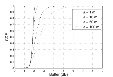
Figure 1: Interference CDF for an REM enabled CR network for several values of $\Delta$ and decorrelation distance, $D_{d}=100$ m.

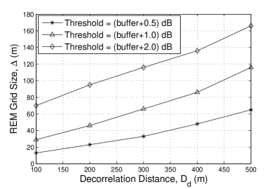
Figure 2: REM grid size, $\Delta$, vs decorrelation distance, $D_{d}$, for different threshold buffer sizes.

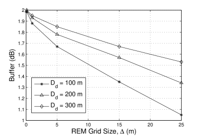
Figure 3: Variation of actual buffer with REM grid size, $\Delta$, for different values of the decorrelation distance, $D_{d}$.

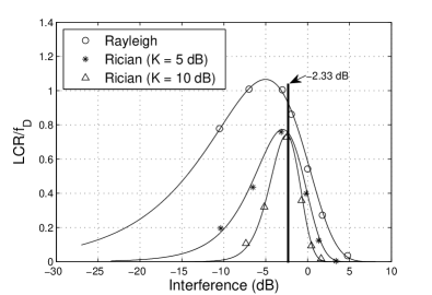
Figure 4: LCR results for different fading conditions. The solid lines represent analytical results. Simulation values are shown by the circle, star and triangle symbols.

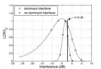
Figure 5: LCR results for the dominant and no dominant interferer cases in a Rayleigh fading scenario. The solid lines represent analytical results. Simulation values are shown by the circle and star symbols.

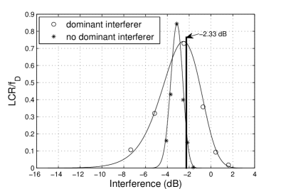
Figure 6: LCR results for the dominant and no dominant interferer cases in a Rician ($K=10$ dB) fading scenario. The solid lines represent analytical results. Simulation values are shown by the circle and star symbols.

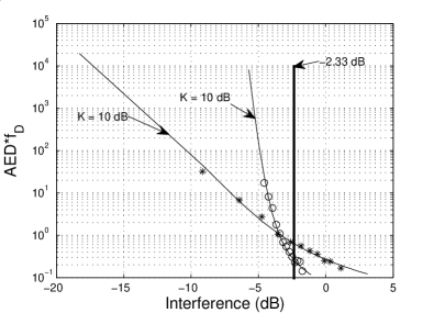
Figure 7: AED results for the dominant and no dominant interferer cases in a Rician ($K=10$ dB) fading scenario. The solid lines represent analytical results. Simulation values are shown by the circle and star symbols.

Throughout the section we assume the following parameter values: shadow fading variance, $\sigma=8$ dB, path loss exponent, $\gamma=3.5$, radius of PU coverage area, $R=1000$ m, radius of CR coverage area, $R_{c}=100$ m, CR density, 1000 CRs per square kilometer, an activity factor of 0.1 and $f_{D}=25$ Hz.

IV-A Imperfections in the REM

In practice, the radio environment is often modeled by dividing an area into a regular grid (typically composed of 100 m $\times$ 100 m grid boxes) and assuming that the fading conditions in any grid box can be approximated by a single point at the center of the box. For example, drive testing of cellular networks to validate path loss models and predicted signal coverage follows this approach. Clearly, larger grid sizes result in errors between measurement and prediction. On the other hand, reducing the grid size results in a large data overhead. Figure 1 shows the cumulative distribution function (CDF) of the magnitude of the actual CR-PU interference when the REM is estimated via a grid size ranging from 1 m $\times$ 1 m to 100 m $\times$ 100 m. The REM approach aims to maintain a 2 dB SINR buffer for the primary, but this is only possible with a perfect REM. When $\Delta=1$ m the 2 dB buffer is nearly achieved but for a grid size of 50 m $\times$ 50 m, the interference exceeds 3 dB for approximately 8% of the time. For a grid size of 100 m $\times$ 100 m, 3 dB is exceeded 30% of the time. In effect this means that if REM information is derived from a coarse grid, the buffer size must be increased or the CRs must back off from the buffer.

The effects of increasing the buffer or backing off the CRs are shown in Figs. 2 and 3 respectively. In Fig. 2 the PU has a target 2 dB buffer but due to the imperfect REM it will not always be achieved. Hence an extra buffer is permitted beyond which the CRs are only allowed, 5% of the time. In Fig. 2 this scenario is denoted by the legend, Threshold = (original + extra) dB. The effects of spatially correlated shadow fading are also considered in Fig. 2. Shadow fading is correlated over any given area and the level of this correlation has a simple effect on the REM grid size. For highly correlated areas a coarse grid (large $\Delta$) will be acceptable whereas in areas of low correlation, a fine grid (small $\Delta$) will be required. Figure 2 shows the REM grid size vs the decorrelation distance of the shadow fading. For a given interference degradation (say the buffer value plus an additional 2 dB) a large decorrelation distance (say 500 m) enables a coarser grid size 165 m $\times$ 165 m relative to a decorrelation distance of 100 m (typical for dense urban areas) when the grid size is 70 m $\times$ 70 m.

In Fig. 3 we consider a back off in the CR allocation policy. In order to meet the nominal 2 dB SINR buffer at least 99% of the time, the CRs have to target a reduced buffer which is less than 2 dB. Figure 3 shows this buffer vs $\Delta$ for various values of $D_{d}$. For a grid size of 25 $\times$ 25 m and a decorrelation distance of 100 m, the interference buffer is 1.05 dB. Figures 2 and 3 are instructive in determining the grid sizes for different radio environments.

IV-B LCR and AED of CR-PU Interference

Figures 4, 5 and 6 show the LCR (normalized by Doppler frequency) of the interference for different types of fading and interference profiles. The interference profiles, i.e., the values of $I_{1},I_{2},\ldots,I_{N}$, are determined for each fading type via a simulation of the CR allocation policy. From 1000 simulations, two sets of interferers are selected. The first set has a dominant interferer and corresponds to the set of interferers with the highest variance. The second set has no dominant interferer and corresponds to the set with the least variance.

For all types of fading, the maximum LCR is observed close to the buffer value. This is because the CR allocation method gives a mean interference level close to the buffer. Even in strong LOS conditions ($K=10$ dB), the interference shows a significant number of level crossings across the buffer due to the scattered component. Figure 5 shows the case of Rayleigh fading where the interference budget is dominated by a single large interferer with a number of smaller additional interferers. Also shown is the case where no dominant interferer exists. Figure 6 shows the same results for a Ricean channel with $K=10$ dB. Figures 5 and 6 show that when there are many small interferers, the resulting interference is more stable compared to the dominant interferer case. Furthermore, the Ricean channel always returns a lower LCR as compared to a Rayleigh channel. The results in Fig. 6 are quite promising. Under the near LOS conditions that may be present with small cell radii, the CR-PU interference has a much lower level crossing rate across the interference buffer for the no dominant interferer case. Hence it may be a desirable part of the CR allocation policy to avoid any single user which takes up a significant part of the buffer. Finally, for completeness, we show the AED results corresponding to Fig. 6. The AED follows from the LCR using standard results [16]. As expected the time spent by the interference above a threshold decreases as the threshold value increases. Therefore, for the no dominant interferer case, the interference seldom crosses the threshold (see Fig. 5), and when it does, it only exceeds the threshold for a small period of time. Finally, we note that all figures show an excellent agreement between the analytical approximations and the simulations.

From the point of view of PU system designers, the following questions are important:

• How much is the CR-PU interference?

• Can it be controlled?

• How often will it exceed a threshold?

• What happens when it does exceed the threshold? Does it stay above for a long time or quickly return back to acceptable levels?

• How do all of the above change with the type of fading?

Figures 4-7 shed an interesting perspective on all the above questions.

V Conclusion

In this paper we have shown that interference degradation to the PU can be significantly underestimated if the channel state information needed to estimate interference levels is derived from a coarse REM. For practical deployments, this may mean that the PU has to accept a much larger interference from the CRs or the CRs may need to set a more conservative interference target. This will reduce the number of CRs allowed. We also determine the LCR and AED for the CR-PU interference and show that the maximum LCR occurs close to the maximum allowed interference level for both Rayleigh and Rician channels. The LCR results show that it is desirable for the interference to be made up of several small interfering CRs rather than a dominant source of interference. The LCR of the former case is more stable than the latter. The AED results also show that the interference exceed the threshold value for small periods of time in the latter case.

References

- [1] “Spectrum Policy Task Force Report (ET Docket-135),” Federal Communications Comsssion, Tech. Rep., 2002. [Online]. Available: http://hraunfoss.fcc.gov/edocs˙public/attachmatch/DOC-228542A1.pdf
- [2] M. A. McHenry, “NSF Spectrum Occupancy Measurements Project Summary,” Shared Spectrum Company, Tech. Rep., 2005.
- [3] M. Vu, N. Devroye, and V. Tarokh, “The primary exclusive regions in cognitive networks,” IEEE Transactions on Wireless Communications, April 2008, submitted.
- [4] M. F. Hanif, M. Shafi, and P. J. Smith, “Interference and deployment issues for cognitive radio systems in shadowing environments,” submitted to the IEEE International Conference on Communications, 2009.
- [5] Y. Zhao, D. Raymond, C. da Silva, J. H. Reed, and S. F. Midkiff, “Performance evaluation of radio environment map-enabled cognitive spectrum-sharing networks,” in Proc. IEEE Military Communications Conference (MILCOM), Oct. 2007, pp. 1–7.
- [6] Y. Zhao, L. Morales, J. Gaeddert, K. K. Bae, J.-S. Um, and J. H. Reed, “Applying radio environment maps to cognitive wireless regional area networks,” in Proc. IEEE International Symposium on New Frontiers in Dynamic Spectrum Access Networks (DySPAN), April 2007, pp. 115–118.
- [7] M. Vu, S. Ghassemzadeh, and V. Tarokh, “Interference in a cognitive network with beacon,” in Proc. IEEE Wireless Comm. and Networking Conf. (WCNC), Apr. 2008, pp. 876–881.
- [8] M. Gudmundson, “Correlation model for shadow fading in mobile radio systems,” IEEE Electronics Letters, vol. 27, no. 23, pp. 2145–2146, 1991.
- [9] N. L. Johnson, S. Kutz, and N. Balakrishnan, Continuous Univariate Distributions, vol. 1, 2nd ed. New York: Wiley, 1995.
- [10] X. Dong and N. C. Beaulieu, “Average level crossing rate and average fade duration of low-order maximal ratio diversity with unbalanced channels,” IEEE Communications Letters, vol. 6, no. 4, pp. 135–137, July 2002.
- [11] P. Ivanis, D. Drajic, and B. Vucetic, “The second order statistics of maximal ratio combining with unbalanced branches,” IEEE Communications Letters, vol. 12, no. 7, pp. 508–510, July 2008.
- [12] R. Barakat, “Level-crossing statistics of aperture-integrated isotropic speckle,” J. Opt. Soc. Amer., vol. 5, pp. 1244–1247, 1988.
- [13] H.-Y. Kim, M. J. Gribbin, K. E. Muller, and D. J. Taylor, “Analytic, computational, and approximate forms for ratios of noncentral and central gaussian quadratic forms,” Journal of Computational and Graphical Statistics, vol. 15, pp. 443–459, June 2006.
- [14] M. Abramowitz and I. A. Stegun, Handbook of Mathematical Functions with Formulas, Graphs, and Mathematical Tables. New York: Dover, 1972.
- [15] R. A. Silverman, “The fluctuation rate of the chi process,” IRE Trans. Inform. Theory, vol. 4, no. 1, pp. 30–34, Mar. 1958.
- [16] G. L. Stuber, Principles of Mobile Communication, 2nd ed. Boston: Kluwer Academic, 2001.