Interference and Deployment Issues for Cognitive Radio Systems in Shadowing Environments

Abstract

In this paper we describe a model for calculating the aggregate interference encountered by primary receivers in the presence of randomly placed cognitive radios (CRs). We show that incorporating the impact of distance attenuation and lognormal fading on each constituent interferer in the aggregate, leads to a composite interference that cannot be satisfactorily modeled by a lognormal. Using the interference statistics we determine a number of key parameters needed for the deployment of CRs. Examples of these are the exclusion zone radius, needed to protect the primary receiver under different types of fading environments and acceptable interference levels, and the numbers of CRs that can be deployed. We further show that if the CRs have apriori knowledge of the radio environment map (REM), then a much larger number of CRs can be deployed especially in a high density environment. Given REM information, we also look at the CR numbers achieved by two different types of techniques to process the scheduling information.

I Introduction

The conventional methodology adopted by spectrum regulatory agencies is to grant exclusive licences to service providers to operate in a particular frequency band. This inflexible approach has led to severe under-utilization of the radio frequency (RF) spectrum.

Such observations have been strengthened by various measurement campaigns [1], [2] whose results have revealed the surprising fact that the scarcity of spectrum is mainly due to the fixed frequency allocation methodology.

The lack of efficient spectrum usage and consumers’ ever-increasing interest in wireless services have triggered a tremendous global research effort on the concept of cognitive radios (CRs) or secondary users (SUs). These CRs are deemed to be intelligent agents capable of making opportunistic use of radio spectrum while simultaneously existing with the legacy primary (licensed) users (PUs) without harming their operation. The enormous interest in the practical deployment of cognitive radios is reflected by the fact that the IEEE has formed a special working group (IEEE 802.22) to develop an air interface for opportunistic secondary access to the TV spectrum.

In addition to ensuring quality of service (QoS) operation, the most important and challenging task for the CRs is to avoid adverse interference to the incumbent PUs. Accurate spectrum sensing capabilities are being developed for CRs and it is envisaged that either individually, or via collaboration, the secondary devices will be able to detect the licensed users with a minimum probability of failure. However, even with the best spectrum sensing techniques the nature of the wireless channel will always result in some interference at the PU due to the CRs. Hence, it is necessary to characterize the nature of the interfering signals along with their impact on the performance of the incumbent licensed users. In addition, the amount of access that CRs are able to obtain without too much impact on the PU is a key issue.

In this paper we focus on the issues described above. Via both analysis and simulations we study the CR access problem and the impact of CRs on the performance of the licensed devices. In particular, we make the following contributions:

• Assuming lognormal shadowing and path loss effects we mathematically characterize the cumulative distribution function (CDF) of the interference due to the cognitive device. Further, we investigate the nature of the distribution of the total interference [3] due to multiple CRs.

• In the same fading conditions we compute primary exclusion zones (PEZ) [4] in which CRs are not permitted to operate. The PEZ approach allows access to CRs when the primary device is willing to pay a price in the form of a reduction in its threshold signal to noise ratio (SNR).

• We determine the permissible number of CRs when the radio environment map (REM) [5] is apriori known to the CRs and we determine how these numbers vary in the different fading environments.

• Finally, we determine the scenarios (CR density, fading parameters) under which REM based CR systems outperform PEZ based cognitive wireless systems.

This paper is organized as follows: Section II describes the system model. Section III derives the CDF of the interference seen by a PU receiver and compares the analytical expression with simulations. We also explore various parameters of the composite interference in a CR network in this section. We introduce the PEZ and REM schemes in Section IV and compare their performance in Section V. Finally, in Section VI we describe our conclusions.

II System Model

Consider a PU receiver in the center of a circular region of radius $R$. The PU transmitter is located uniformly in an annulus of outer radius $R$ and inner radius $R_{0}$ centered on the PU receiver. It is to be noted that we place the PU receiver at the center only for the sake of mathematical convenience (see Fig. 1). The use of the annulus restricts devices from being too close to the receiver. This matches physical reality and also avoids problems with the classical inverse power law relationship between signal strength and distance [6]. In particular, having a minimum distance, $R_{0}$, prevents the signal strength from becoming infinite as the transmitter approaches the receiver. Similarly, we assume that multiple CR transmitters are uniformly located in the annulus. At any given time, each CR has a probability of seeking a connection, given by the activity factor, $p$. The number of CRs wishing to operate is denoted $N_{CR}$. Of these CRs, a certain number will be accepted depending on the allocation mechanism. Hence, a random number of CRs denoted $N\leq N_{CR}$ will transmit during the PU transmission and create interference at the PU receiver.

The received signal strength for both the PU transmitter to PU receiver and CR transmitter to PU receiver is assumed to follow the classical distance dependent, lognormal shadowing model. For a generic interferer, this is given by

$$I=BLr^{-\gamma}=B10^{\tilde{X}/10}r^{-\gamma}=Be^{X}r^{-\gamma}$$ (1)

where $r$ is the random distance from the transmitter to the receiver, $\gamma$ is the path loss exponent (normally in the range of 2 to 4) and $L$ is a shadow fading variable. The lognormal variable, $L$, is given in terms of the zero mean Gaussian, $\tilde{X}$, which has standard deviation $\sigma$ (dB) and $X=\beta\tilde{X}$ where $\beta=\ln(10)/10$. The standard deviation of $X$ is denoted by $\sigma_{x}$. The constant $B$ is determined by the transmit power. The desired primary signal strength, $S$, has the same form, with a different transmit power, so that $S=AL_{p}r_{p}^{-\gamma}$. Note that all the links are assumed to be independent and identically distributed (i.i.d.) so that spatial correlation is ignored. The results in the paper can be further generalized to more realistic scenarios by considering the system models such as those presented in [7, 8].

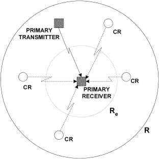
Figure 1: System model ($R_{0}$ not shown)

III Statistical Characterization of Interference at the Primary Receiver

In this section we investigate the interference at the PU receiver due to one or more CRs. Firstly we characterize the interfering signal, given in (1), by computing the CDF, $F_{I}(x)=P(I<x)$. This can be done as follows:

$$F_{I}(x) {}={} P\big{(}Be^{X}r^{-\gamma}<x\big{)}$$ (2)

$${}={} P\Bigg{(}e^{-X}r^{\gamma}>\frac{B}{x}\Bigg{)}$$

$${}={} P(e^{U}r^{\gamma}>y)$$

$${}={} E_{U}\Big{(}P\Big{(}r>y^{\frac{1}{\gamma}}e^{\frac{-U}{\gamma}}\Big{)}\Big{)}$$

$${}={} E_{U}\Big{(}1-F_{R}\Big{(}y^{\frac{1}{\gamma}}e^{\frac{-U}{\gamma}}\Big{)}\Big{)}$$

In (2), $U=-X$, $E_{U}$ represents expectation over the random variable $U$ and $y=B/x$. To evaluate the expectation in (2) we note that the CDF of $r$ is given by:

$$F_{R}(r)=\frac{r^{2}-R_{0}^{2}}{R^{2}-R_{0}^{2}},\qquad R_{0}\leq r\leq R.$$

Using this CDF, (2) can be rewritten as:

$$F_{I}(x)=E_{U}(G_{R}(y)),$$ (3)

where

$$G_{R}(y)=\left\{\begin{array}[]{ll}0&\textrm{$u<w_{0}$}\\ \bigg{(}\frac{R^{2}-y^{\frac{2}{\gamma}}e^{\frac{-2u}{\gamma}}}{R^{2}-R_{0}^{2}}\bigg{)}&\textrm{$w_{0}<u<w_{1}$}\\ 1&\textrm{$u>w_{1}$}\end{array}\right.$$ (4)

and $w_{0}=\ln(yR^{-\gamma})$, $w_{1}=\ln(yR_{0}^{-\gamma})$. Since $U=-X$ is Gaussian, $U\sim\mathcal{N}(0,\sigma_{x}^{2})$, the CDF, $F_{I}(x)=E_{U}(G_{R}(y))$, becomes:

$$F_{I}(x) {}={} \int_{w_{0}}^{w_{1}}\!\!\!\frac{R^{2}-y^{\frac{2}{\gamma}}e^{\frac{-2u}{\gamma}}}{R^{2}-R_{0}^{2}}f(u)du+\int_{w_{1}}^{\infty}\!\!f(u)du$$ (5)

$${}={} \frac{R^{2}}{(R^{2}-R_{0}^{2})\sqrt{2\pi\sigma_{x}^{2}}}\int_{w_{0}}^{w_{1}}\!\!\!e^{\frac{-u^{2}}{2\sigma_{x}^{2}}}du$$

$${-}\>\frac{(\frac{B}{x})^{2/\gamma}}{(R^{2}-R_{0}^{2})\sqrt{2\pi\sigma_{x}^{2}}}\int_{w_{0}}^{w_{1}}\!\!\!e^{\frac{-2u}{\gamma}-\frac{-u^{2}}{2\sigma_{x}^{2}}}du$$

$${+}\>\frac{1}{\sqrt{2\pi\sigma_{x}^{2}}}\int_{w_{1}}^{\infty}\!\!\!e^{\frac{-u^{2}}{2\sigma_{x}^{2}}}du.$$

All the integrals in (5) can be written in terms of integrals of Gaussian PDFs. Hence (5) can be written as shown in (6), where $F_{Z}(.)$ is the CDF of a standard Gaussian.

$$F_{I}(x) =1-F_{Z}\Bigg{(}\frac{w_{1}}{\sigma_{x}}\Bigg{)}+\frac{1}{R^{2}-R_{0}^{2}}\Bigg{[}\Bigg{\{}R^{2}F_{Z}\Big{(}\frac{w_{1}}{\sigma_{x}}\Big{)}-R^{2}F_{Z}\Big{(}\frac{w_{0}}{\sigma_{x}}\Big{)}\Bigg{\}}$$ (6)

$$-\Big{(}\frac{B}{x}\Big{)}^{\frac{2}{\gamma}}e^{\big{(}\frac{2\sigma_{x}^{2}}{\gamma^{2}}\big{)}}\Bigg{\{}F_{Z}\Bigg{(}\frac{w_{1}+2\sigma_{x}^{2}/\gamma}{\sigma_{x}}\Bigg{)}-F_{Z}\Bigg{(}\frac{w_{0}+2\sigma_{x}^{2}/\gamma}{\sigma_{x}}\Bigg{)}\Bigg{\}}\Bigg{]}$$

In order to validate the CDF given in (6), we compare the results of this expression with the CDF obtained using Monte Carlo simulation as shown in Fig. 2. It can be seen that the analytical and simulated interference CDFs agree over a wide range of propagation parameters. The discrepancy between the analytical and simulated curves in the tail region is due to the limited number of realizations used and the inherent long tailed properties of the lognormal. Hence, a complete characterization of the interference due to a single CR is possible. Next, we consider multiple CRs. In cognitive wireless networks the PU device under consideration may be affected by the interference due to many CRs. In this case, the total interference, denoted $I_{TOT}$, is given by:

$$I_{TOT}=\sum_{i=1}^{N}Be^{X_{i}}r_{i}^{-\gamma}=\sum_{i=1}^{N}BL_{i}r_{i}^{-\gamma},$$ (7)

where the parameters are as defined in (1). Equation (7) is a random sum of a finite number of lognormals with each lognormal being multiplied by a random distance factor. Problems similar to this, but involving a non random sum without incorporating the random distance factor, have been tackled in the past [9, 10, 11, 12, 13, 14]. Historically, lognormal approximations to this summation have been envisaged. Approximations are definitely required since although (6) gives an analytical result for a single interferer, it is too complex to allow an exact approach for sums of interferers. Hence one is tempted to use the same lognormal approximation for (7). However, we show that lognormal approximations are not accurate. For convenience, consider a lognormal approximation to a single interferer, $I$, of the form given in (1). Let the moments of $I$ be denoted by $E(I^{j})=m_{j}$. We seek to approximate $I$ with the lognormal $Y=e^{Z}$ where $Z\sim\mathcal{N}(\mu_{z},\sigma_{z}^{2})$. The simplest approach to fitting $Y$ is via the Fenton-Wilkinson approximation [15, 9] which computes the first two moments, so that:

$$E(Y^{k})=E(I^{k}),\quad k=1,2$$ (8)

Hence, the lognormal approximation has perfect moments up to order 2. To demonstrate the lack of fit we consider the skewness of $Y$ and $I$ which also involves the third moment. For any lognormal, say $Y$, the third moment is related to the first two by:

$$E(Y^{3})=\Bigg{(}\frac{E(Y^{2})}{E(Y)}\Bigg{)}^{3}.$$ (9)

Now, consider the skewness of $I$,

$$SK(I) {}={} \frac{E[(I-m_{1})^{3}]}{(m_{2}-m_{1}^{2})^{3/2}}$$ (10)

$${}={} \frac{m_{3}+2m_{1}^{3}-3m_{1}m_{2}}{(m_{2}-m_{1}^{2})^{3/2}}.$$

Similarly, the skewness of $Y$ can be written as:

$$SK(Y) {}={} \frac{E(Y^{3})+2E(Y)^{3}-3E(Y)E(Y^{2})}{(E(Y^{2})-E(Y)^{2})^{3/2}}$$ (11)

$${}={} \frac{E(Y^{3})+2m_{1}^{3}-3m_{1}m_{2}}{(m_{2}-m_{1}^{2})^{3/2}}$$

Hence, the lognormal approximation is more skewed than the real interference if $E(Y^{3})>m_{3}$. Now, consider

$$\frac{E(Y^{3})}{m_{3}} {}={} \frac{(m_{2}/m_{1})^{3}}{m_{3}}$$ (12)

$${}={} \frac{\bigg{(}\frac{B^{2}E(e^{2X})E(r^{-2\gamma})}{BE(e^{X})E(r^{-\gamma})}\bigg{)}^{3}}{B^{3}E(e^{3X})E(r^{-3\gamma})}$$

$${}={} \frac{\bigg{(}\frac{E(e^{2X})}{E(e^{X})}\bigg{)}^{3}}{E(e^{3X})}\frac{\bigg{(}\frac{E(r^{-2\gamma})}{E(r^{-\gamma})}\bigg{)}^{3}}{E(r^{-3\gamma})}$$

$${}={} \frac{\bigg{(}\frac{E(r^{-2\gamma})}{E(r^{-\gamma})}\bigg{)}^{3}}{E(r^{-3\gamma})}.$$

The above results follow since (9) also holds for the lognormal $e^{X}$. The moments of $r$ in (12) can be found as:

$$E(r^{-k\gamma})=\frac{2(R^{2-k\gamma}-R_{0}^{2-k\gamma})}{(R^{2}-R_{0}^{2})(2-k\gamma)}.$$ (13)

Equation (13) is obtained using $f(r)=\frac{2r}{(R^{2}-R_{0}^{2})}$ as the PDF for the CR distance in the annulus $R_{0}<r<R$. For large $R$ (1000 m in our case), small $R_{0}$ (we use 1m) and with $\gamma\geq 3$, (13) gives:

$$E(r^{-k\gamma})\approx\frac{-1}{R^{2}}\bigg{(}\frac{2}{2-k\gamma}\bigg{)}=\frac{2}{R^{2}(k\gamma-2)}.$$ (14)

Thus, the ratio of the moments in (12) becomes:

$$\frac{E(Y^{3})}{m_{3}} {}\approx{} \bigg{(}\frac{\gamma-2}{2\gamma-2}\bigg{)}^{3}\frac{R^{2}(3\gamma-2)}{2}$$ (15)

It can be observed from the above expression that for typical values of the parameters, $E(Y^{3})>>m_{3}$, and the ratio is of the order of $R^{2}$. Thus the equivalent lognormal will be massively more skewed than the real interference. Now as skewness is a key shape determining factor (especially in the tails), the simple lognormal approximation will not be accurate. Note that this large discrepancy in skewness is due to the random distance factors. Exactly the same conclusions are reached when attempting to fit sums of interferers. Hence, it appears that a simple lognormal approximation will not suffice and further research is required. In one possible approach [3] has approximated the total interference of the form given in (7) with a more flexible shifted three parameter lognormal random variable using cumulant matching. Comparison between the simulation results and this approximation shows good matching especially in the head portion of the CDF. Similarly, the recent work in [16] analyzes the aggregate interference in the absence of any shadow fading. This makes it difficult to compare the two sets of results. In this paper, we use simulations to assess the REM and PEZ schemes as discussed in Section IV.

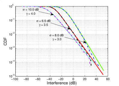
Figure 2: A comparison of analytical and simulated CDFs of interference over a range of propagation parameters.

IV REM And PEZ Based Schemes

In all simulations CRs are located uniformly in the primary coverage area. The number of active CRs, $N_{CR}$, is binomially distributed with a maximum number of CRs given by $\pi R^{2}D_{CR}$, where $D_{CR}$ is the density of the CRs (number of CRs per $\text{m}^{2}$) and we ignore the negligible hole in the circle of radius $R_{0}$. The binomial probability that a CR wishes to transmit is given by the activity factor, $p=0.1$. The primary receiver is at the center of the coverage area and the primary transmitter is also uniformly located in the primary coverage area. In this section we consider two fundamentally different schemes for managing the interference at the PU receiver. The REM approach utilizes instantaneous knowledge of all the interference values whereas the PEZ approach only uses average information. Assume there are $N_{CR}$ CR transmitters which desire a connection. Each of the $N_{CR}$ CRs has an interference power at the primary receiver given by (1) and denoted $I_{1},I_{2},\ldots,I_{N_{CR}}$. Based on these interference values, the REM and PEZ approaches are described below.

IV-A REM Approach

The REM approach [5] assumes that $I_{1},I_{2},\ldots,I_{N_{CR}}$ are known and selects those CRs for transmission which satisfy an SINR constraint. The constraint chosen is that the added interference must not decrease the SNR by more than $\Delta$ dB. For example, if SNR = 10 dB in the absence of CRs, then those CRs chosen must give $\text{SINR}\geq(10-\Delta)$ dB. Two methods are chosen for selection, a centralized approach and a decentralized approach.

IV-A1 Centralized Selection

Here we assume that a centralized controller knows $I_{1},I_{2},\ldots,I_{N_{CR}}$ instantaneously and creates a list of the ordered interferers as $I_{(1)}\leq I_{(2)}\leq\ldots\leq I_{(N_{CR})}$. The first $n$ CRs are selected such that $\sum_{i=1}^{n}I_{(i)}\leq\Delta$ dB and $\sum_{i=1}^{n+1}I_{(i)}>\Delta$ dB.

IV-A2 Decentralized Selection

Here we assume that the CRs are considered in their original order which can be interpreted as their order of arrival. Each interferer is considered in turn and is accepted if the combined interference from previously accepted CRs and the current CR is less than $\Delta$ dB. If a CR is not accepted, the next CR in the list is investigated.

IV-B PEZ Approach

The REM approach uses a detailed REM to give information about the interference resulting from any CR. In contrast, the PEZ approach [4] only uses location information to control the access of CRs. A simple exclusion zone is created with radius $R_{e}$ around the primary receiver. No CR is allowed to transmit inside the PEZ and all CRs outside the PEZ are permitted. The radius, $R_{e}$, is set so that the SINR within the PU coverage area is degraded by a certain amount. Specifically, the primary coverage area is defined to give an SNR greater than 5 dB, 95% of the time. By allowing CRs to operate we accept a new SINR target, less than 5 dB, which is achieved at least 95% of the time.

V Simulation Results

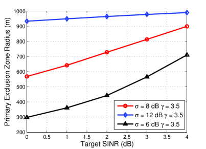
Figure 3: The effect of $\sigma$ and the target SINR on the PEZ radius for a medium density of CRs.

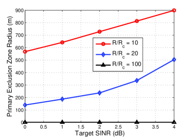
Figure 4: PEZ radius vs target SINR for different values of the ratio of primary to secondary device coverage areas ($\sigma=8$ dB, $\gamma=3.5$).

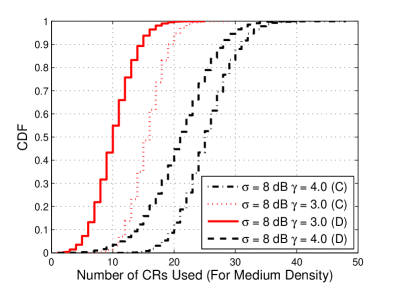
Figure 5: CDF of the number of CRs obtained using REM based approaches for various $\gamma$ values. D and C denote decentralized and centralized approaches.

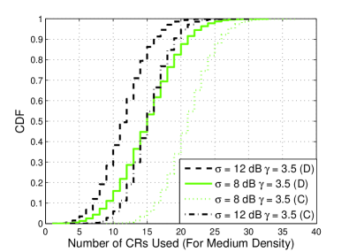
Figure 6: CDF of the number of CRs obtained using REM based approaches for various $\sigma$ values. D and C denote decentralized and centralized approaches.

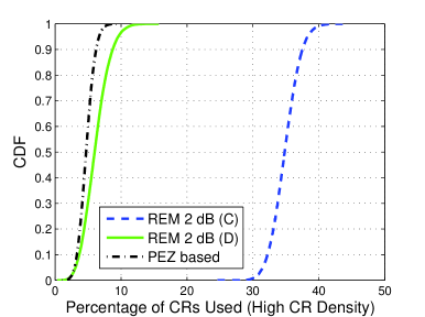
Figure 7: Percentage of CRs given access for a high CR density ($\sigma=8$ dB, $\gamma=3.5$).

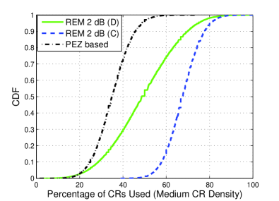
Figure 8: Percentage of CRs given access for a medium CR density ($\sigma=8$ dB, $\gamma=3.5$).

We assume a PU coverage radius of $R=1000$ m, and the transmit power is adjusted such that the SNR in the coverage area exceeds 5 dB with probability 0.95. In other words the area reliability with a 5 dB target is 95%. The CR transmit power is also chosen so that 5 dB is achieved at least 95% of the time for a given CR coverage radius, $R_{c}$. We take $R_{0}=1$ m. Two kinds of CR penetration densities were chosen, a high density of 10,000 CRs per sq. km and a corresponding moderate density of 1000 CRs per sq. km. Additionally, it was assumed that only 10% of the CRs wish to be active at any one time. The values of the propagation constants, $\gamma$ and $\sigma$ are given on the relevant figures.

V-A Exclusion Zone Results

Given a variety of target SINRs, Fig. 3 shows the PEZ radius for different values of $\sigma$. For example, if the interference degrades the target SNR from 5 dB to an SINR of 4 dB, then the PEZ radius is approximately 700 m, for $\sigma=6$ dB and $\gamma=3.5$. It is interesting to note that the PEZ radius excludes virtually the entire PU coverage area for all target SINRs in [0-5] dB when $\sigma=12$ dB, corresponding to dense urban areas. This result implies that for a given target SINR, environments with larger $\sigma$ will result in higher interference and an increased $R_{e}$. This observation is consistent with previous observations reported in [17].

Increasing the CR transmit power or increasing $R_{c}$ will correspondingly increase the interference and hence the PEZ radius. Figure 4 shows the PEZ radius vs target SINR for three different values of $R/R_{c}$. These calculations were done for $\sigma=8$ dB and $\gamma=3.5$. Reducing the CR transmit power will obviously result in a lower PEZ radius.

V-B Numbers of CRs

Figures 5 and 6 show CDFs of the number of CRs for the two different types of REM approach and the impact of varying the fading parameters. In both these figures, the centralized approach is superior, since it is designed to pick up the maximum number of CRs that aggregate to make up the acceptable interference degradation. We also note from Fig. 5 that increasing $\gamma$ increases the number of permissible CRs. This is because environments where $\gamma=4$ will experience less interference compared to environments where $\gamma=3$ due to increased path loss. Looking at Fig. 6, increasing $\sigma$ decreases the permissible number of CRs. This result reinforces the conclusion of Fig. 3 where increasing $\sigma$ increased the PEZ radius - effectively reducing the area in which CRs operate and also reducing the permissible number of CRs. Note that dense urban environments are characterized by $\gamma$ values of 4 and above and $\sigma$ values of 8 dB and above. These two parameters have opposing effects on the permissible number of CRs.

Figure 7 compares the PEZ and REM approaches in terms of the percentage of CRs that gain access in a high density environment. The centralized approach is far superior, showing the advantage gained if the CR knows the radio environment. This advantage is dissipated by the decentralized approach as effectively a few CRs consume the permissible interference budget (2 dB in this case). The PEZ approach is worse than the decentralized strategy. It is an important result that the decentralized REM approach, which can be thought of as a first-come-first-served mechanism, results in better access for the CRs than the PEZ approach. Hence, the overhead of obtaining the REM can result in improved access. It is critical that the REM information be used in an intelligent allocation process. Figure 8 revisits the results in Fig. 7 for a lower CR density. Here too the centralized approach is better, but now the decentralized approach shows an even bigger advantage over the PEZ approach for higher values of the CDF.

The results in Figs. 5-8 taken collectively are the key contribution of this paper. They clearly show the advantage in terms of permissible CR numbers if a knowledge of the radio environment is made available to the CRs. Furthermore, they show that the full REM gains are only obtained if a smart access control algorithm is used which chooses many CRs with low interference instead of a few stronger interferers which might subsume the interference budget.

VI Conclusion

The interference due to a single CR can be characterized in closed form for the scenario considered. However, the total interference due to multiple CRs is more difficult. Simple lognormal approximations are shown to be inaccurate and more complex models are required. Two interference management approaches have been considered based on REM and PEZ ideas. The REM approach requires considerable higher overheads but can perform substantially better than the PEZ approach. To achieve substantial gains an intelligent allocation method is, however, essential.

References

- [1] “Spectrum Policy Task Force Report (ET Docket-135),” Federal Communications Comsssion, Tech. Rep., 2002. [Online]. Available: http://hraunfoss.fcc.gov/edocs˙public/attachmatch/DOC-228542A1.pdf
- [2] M. A. McHenry, “NSF Spectrum Occupancy Measurements Project Summary,” Shared Spectrum Company, Tech. Rep., 2005.
- [3] A. Ghasemi and E. S. Sousa, “Interference aggregation in spectrum-sensing cognitive wireless networks,” IEEE Journal of Selected Topics in Signal Processing, vol. 2, pp. 41–56, Feb. 2008.
- [4] M. Vu, N. Devroye, and V. Tarokh, “The primary exclusive regions in cognitive networks,” IEEE Transactions on Wireless Communications, April 2008, submitted.
- [5] Y. Zhao, D. Raymond, C. da Silva, J. H. Reed, and S. F. Midkiff, “Performance evaluation of radio environment map-enabled cognitive spectrum-sharing networks,” in Proc. IEEE Military Communications Conference (MILCOM), Oct. 2007, pp. 1–7.
- [6] M. Vu, S. Ghassemzadeh, and V. Tarokh, “Interference in a cognitive network with beacon,” in Proc. IEEE Wireless Comm. and Networking Conf. (WCNC), Apr. 2008, pp. 876–881.
- [7] Y. Chen, C. Yuen, Y. Zhang, and Z. Zhang, “Cross-correlation analysis of generalized distributed antenna systems with cooperative diversity,” in Proc. IEEE Vehicular Technology Conference (VTC), April 2007, pp. 309–313.
- [8] ——, “Diversity gains of generalized distributed antenna systems with cooperative users,” in Proc. IEEE Wireless Communications and Networking Conference (WCNC), March 2007, pp. 797–802.
- [9] A. Abu-Dayya and N. C. Beaulieu, “Outage probabilities in the presence of correlated lognormal interferers,” IEEE Trans. Veh. Technol., vol. 43, pp. 164–173, Feb. 1994.
- [10] N. C. Beaulieu, A. Abu-Dayya, and P. McLance, “Estimating the distribution of a sum of independent lognormal random variables,” IEEE Trans. Commun., vol. 43, pp. 2869–2873, Dec. 1995.
- [11] N. C. Beaulieu and Q. Xie, “An optimal lognormal approximation to lognormal sum distributions,” IEEE Trans. Veh. Technol., vol. 53, pp. 479–489, Mar. 2004.
- [12] N. B. Mehta, J. Wu, A. F. Molisch, and J. Zhang, “Approximating a sum of random variables with a lognormal,” IEEE Transactions on Wireless Communications, vol. 6, no. 7, pp. 2690–2699, July 2007.
- [13] M. D. Renzo, F. Graziosi, and F. Santucci, “A general formula for log-mgf computation: Application to the approximation of log-normal power sum via Pearson type IV distribution,” in IEEE Vehicular Technology Conference, May 2008, pp. 999–1003.
- [14] Z. Liu, J. Almhana, and R. McGorman, “Approximating lognormal sum distributions with power lognormal distributions,” IEEE Transactions on Vehicular Technology, vol. 57, no. 4, pp. 2611–2617, July 2008.
- [15] L. F. Fenton, “The sum of lognormal probability distributions in scatter transmission systems,” IRE Trans. Commun. Syst, vol. CS-8, pp. 57–67, 1960.
- [16] N. S. Shankar and C. Cordeiro, “Analysis of aggregated interference at DTV receivers in TV bands,” in Proc. IEEE Cognitive Radio Oriented Wireless Networks and Communications (CrownCom), May 2008, pp. 1–6.
- [17] A. M. Viterbi and A. J. Viterbi, “Erlang capacity of a power controlled CDMA system,” IEEE J. Select. Areas Communications, vol. 11, no. 6, pp. 892–900, Aug. 1993.