Homogeneous photometry and star counts in the field of 9 Galactic star clusters

Abstract

We present homogeneous $V,I$ CCD photometry of nine stellar fields in the two inner quadrants of the Galactic plane. The lines-of-view to most of these fields aim in the direction of the very inner Galaxy, where the Galactic field is very dense, and extinction is high and patchy. Our nine fields are, according to several catalogs, centred on Galactic star clusters, namely Trumpler 13, Trumpler 20, Lynga 4, Hogg 19, Lynga 12, Trumpler 25, Trumpler 26, Ruprecht 128, and Trumpler 34. Apart from their coordinates, and in some cases additional basic data (mainly from the 2MASS archive), their properties are poorly known. By means of star count techniques and field star decontaminated Color-Magnitude diagrams, the nature and size of these visual over-densities has been established; and, when possible, new cluster fundamental parameters have been derived. To strengthen our findings, we complement our data-set with JHK_s photometry from the 2MASS archive, that we analyze using a suitably defined Q-parameter.
Most clusters are projected towards the Carina-Sagittarium spiral arm. Because of that, we detect in the Color Magnitude Diagrams of most of the other fields several distinctive sequences produced by young population within the arm. All the clusters are of intermediate or old age. The most interesting cases detected by our study are, perhaps, that of Trumpler 20, which seems to be much older than previously believed, as indicated by its prominent -and double- red clump; and that of Hogg 19, a previously overlooked old open cluster, whose existence in such regions of the Milky Way is puzzling.

Table 1: Basic parameters of the clusters under investigation. Coordinates are for J2000.0 equinox

Label	Name	$RA$	$DEC$	$l$	$b$	$E(B-V)_{FIRB}$
		$hh:mm:ss$	o : ′ : ′′	[deg]	[deg]	mag
1	Trumpler 13	10:23:48	-60:08:00	285.515	-2.353	1.74
2	Trumpler 20	12:39:34	-60:37:23	301.475	+2.221	1.10
3	Lynga 4	15:33:19	-55:14:00	324.656	+0.659	6.88
4	Hogg 19	16:28:57	-49:06:00	335.088	-0.302	9.32
5	Lynga 12	16:46:04	-50:46:00	335.695	-3.463	1.06
6	Trumpler 25	17:24:29	-39:01:00	339.156	-1.774	1.74
7	Trumpler 26	17:28:33	-29:30:00	357.524	+2.840	1.46
8	Ruprecht 128	17:44:18	-34:53:00	354.778	-2.864	1.05
9	Trumpler 34	18:39:48	-08:25:00	24.119	-1.264	2.81

1 Introduction

This study is a continuation of our homogeneous photometric survey for neglected open clusters in the inner Galaxy. The main motivations of this survey are twofold:

1. We are searching for old and intermediate age clusters inside the solar ring in order to extend the baseline of the radial abundance gradient in the disk, and this way contribute to better understand our galaxy’s chemical evolution. In spite of this being a notoriously difficult to observe region -due to the extreme density of the Galactic disk field, the presence of the bulge, and the highly variable extinction- we have been able to unravel several intermediate-age clusters (Carraro et al. 2005a, 2005b, 2006), which we aim to follow up spectroscopically to measure their metallicity. The present observations will also allow to study the rate of cluster formation and dissolution in hostile regions of our galaxy such as the above.

2. We are looking for young clusters and/or spiral features in order to better trace the location and extent of the inner Galaxy spiral arms Carina-Sagittarius and Scutum-Crux, and probe the existence of a more distant arm beyond Carina (see Carraro & Costa 2009, Baume et. al 2009).

In this paper we focus on 9 additional fields centred on catalogued open clusters (Dias et al. 2002): Trumpler 13, Trumpler 20, Lynga 4, Hogg 19, Lynga 12, Trumpler 25, Trumpler 26, Ruprecht 128, and Trumpler 34. Apart from their coordinates (listed in Table 1), and in some cases additional basic data (discussed in Section 3), their properties are poorly known. In the same Table 1 we report the reddening in the direction of our targets, as provided by Schlegel et al. (1998). This represents the extinction all the way to infinity, and is only meant to provide an indication of the upper value we expect for the reddening.

The layout of the paper is as follows. In Sect. 2 we provide details on our observations and data reduction procedure. In Sect. 3 we summarize previous results (if any) for the fields under study. Sects. 4 and 5 are dedicated to star counts, necessary for the field star decontamination process, and to determine the structure and extension of each over-density. To this aim, we make use both of our data-set and of photometric data from the 2MASS archive (Skrutskie et al. 2006). In Sect. 6. we discuss the Color-Magnitude Diagram (CMD) of each over-density, and provide estimates of the fundamental parameters of those recognized as star clusters. Finally, in Sect. 7 we summarize our results.

1.1 Observations

The observations were made with a cassegrain focus CCD Imager attached to the 0.9m telescope at Cerro Tololo Inter-American Observatory (CTIO). This camera is equipped with a Tektronic 2048$\times$2046 CCD detector with 24$\mu$ pixels, yielding a nominal scale of 0.396 ^′′/pixel and a field-of-view (FOV) of $13.5\mbox{${}^{\prime}$}\times 13.5\mbox{${}^{\prime}$}$. Gain and readout noise were 1.5 e^-/ADU and 3.6 e^-, respectively. QE and other detector characteristics can be found at the dedicated webpage.

The observational material was obtained in two observing runs (April and June, 2006), summarized in Tables 2 and 3. Both runs were blessed by photometric conditions and an average seeing of 1.1^′′.

Table 2: Log of photometric observations on April 19, 2006.

Cluster	Filter	Exp time (sec)	Airmass
Lynga 4	V	2x5, 30, 600	1.03-1.24
	I	5, 10, 30, 600	1.05-1.27
Trumpler 13	V	2x5, 30, 600	1.14-1.30
	I	5, 10, 30, 600	1.12-1.26
Trumpler 20	V	2x5, 30, 2x600	1.20-1.40
	I	5, 10, 30, 2x600	1.17-1.35

Table 3: Log of photometric observations on June 27-28, 2006.

Cluster	Date	Filter	Exp time (sec)	Airmass
Hogg 19	Jun 27	V	2x5, 2x10, 2x600	1.03-1.20
		I	2x5, 2x10, 600	1.03-1.20
Lynga 12		V	2X5, 2X10, 30, 600	1.15-1.24
		I	2x5, 2x10, 30, 600	1.16-1.26
Trumpler 25		V	2x5, 2x10, 30, 600	1.09-1.33
		I	2x5, 2x10, 30, 600	1.12-1.30
Trumpler 26	Jun 28	V	3x5, 3x10, 2x600	1.03-1.54
		I	3x5, 3x10, 2x600	1.08-1.50
Ruprecht 128		V	3x5, 3x10, 2x600	1.11-1.64
		I	3x5, 3x10, 2x600	1.15-1.60
Trumpler 34		V	3x5, 3x10, 2x600	1.03-1.84
		I	3x5, 3x10, 2x600	1.08-1.80

The nine areas observed are shown in Fig. 1. Numbers on the upper-left corners indicate the cluster label, in agreement with Table 1. North is up and East to the left. FOV is 13.5^′ on a side. Finders were made from 600 sec $V$-band frames.

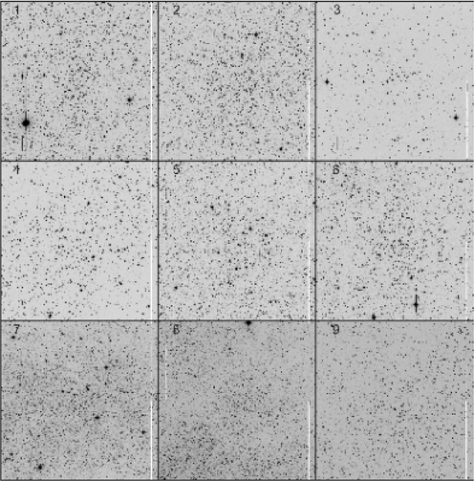
Figure 1: Observed areas . Numbers in the upper-left corners indicate the cluster label, in agreement with Table 1. North is up and East to the left. FOV is 13.5^′ on a side. Finders were made from 600 sec $V$-band frames.

Our $VRI$ instrumental photometric system was defined by the use of the default $VRI$ Johnson-Kron-Cousins set available for broad-band photometry on the CTIO 0.9m telescope. Additional information about them, including their transmission curves, can be found following this link .

Five $UBVRI$ standard star areas from the catalog of Landolt (1992) were observed multiple times each night to determine the transformation of our instrumental magnitudes to the standard $VRI$ system. A few of the standard areas were followed each night up to about 2.2 airmasses to optimally determine atmospheric extinction. Although most of the areas observed include stars of a variety of colors, a few red standards were observed additionally.

1.2 Reductions

Basic calibration of the CCD frames was done using the IRAF package CCDRED. For this purpose, zero-exposure frames and twilight sky flats were taken every night. Photometry was performed using the IRAF DAOPHOT and PHOTCAL packages, and instrumental magnitudes were extracted following the point spread function (PSF) method (Stetson 1987). The PSF photometry was aperture-corrected -filter by filter- using aperture corrections determined performing aperture photometry on a suitable number (typically 15 to 20) of bright stars in the fields. These corrections were found to vary from 0.08 to 0.21 magnitudes, depending on filter.

1.3 The photometry

In our April 2006 run a grand-total of 187 individual standard star observations were secured, and we obtained a photometric solution of the form:

$v=V+(2.055\pm 0.003)+(0.15\pm 0.01)\times X+(0.017\pm 0.002)\times(V-I)$
$i=I+(2.945\pm 0.002)+(0.06\pm 0.01)\times X+(0.027\pm 0.002)\times(V-I)$ ,

Given the very stable photometric conditions encountered in our June 2006 run, a single photometric solution was derived for all two nights. From a grand-total of 179 individual standard star observations we obtained:

$v=V+(2.079\pm 0.003)+(0.16\pm 0.01)\times X+(0.024\pm 0.002)\times(V-I)$
$i=I+(2.994\pm 0.003)+(0.08\pm 0.01)\times X+(0.032\pm 0.002)\times(V-I)$ ,

For both runs, the final r.m.s of the fitting turned out to be 0.020 and 0.022 for the $V$ and $I$ the pass-bands, respectively.

Global photometric errors were estimated using the scheme developed by Patat & Carraro (2001, Appendix A1), which takes into account the errors resulting from the PSF fitting procedure (i.e. from ALLSTAR), and the calibration errors (corresponding to the zero point, color terms and extinction errors). In Fig. 2 we present global photometric error trends plotted as a function of $V$ magnitude. Quick inspection shows that most stars brighter than $V\approx 20$ mag have errors lower than 0.20 mag in magnitude and lower than 0.25 mag in color. The final photometric catalog will be made available at the WEBDA database .

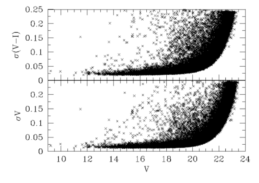
Figure 2: Photometric errors in $V$ and $(V-I)$, plotted as a function of $V$ magnitude

Completeness corrections were determined by means of artificial-star experiments on our data. We created artificial images of each field by adding artificial stars in random positions to the original images. The artificial stars had the same color and luminosity distribution as the original sample. In order to avoid the creation of overcrowding, a maximum of 15$\%$ of the original number of stars was added (between 1000-5000 objects, depending on stellar density). In this way we found that our completeness level is better than 50$\%$ down to $V$ = 20.5. We have adopted this latter figure to run our field star decontamination procedure (see Sect. 5).

1.4 Comparison with previous studies

We compared our photometry with previous studies. The only case for which it was possible is Trumpler 20 (see next Section), which we compared with Platais et al. (2009). These authors report BVI photometry of $\sim$ 2500 stars in a field of $20^{\prime}\times 20^{\prime}$ centreed on the cluster. The two studies have different spatial coverage and depth, being our study deeper but confined to a smaller area.
We cross-identified the two photometric catalogues and found 2009 stars in common. From the comparison we obtain:

$$\Delta V=0.019\pm 0.009$$ (1)

and,

$$\Delta(V-I)=0.024\pm 0.012.\\$$ (2)

These results show that the two studies agree, since no sizable zero-points offsets are found.

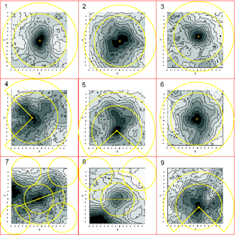
Figure 3: Surface Density Maps for the nine fields under study. Numbers in the upper-left corners indicate the cluster label, in agreement with Table 1. They have been constructed using a 300-pixel kernel half-width and a grid of 25-pixel cells. Red squares indicate the whole field. See text for more details

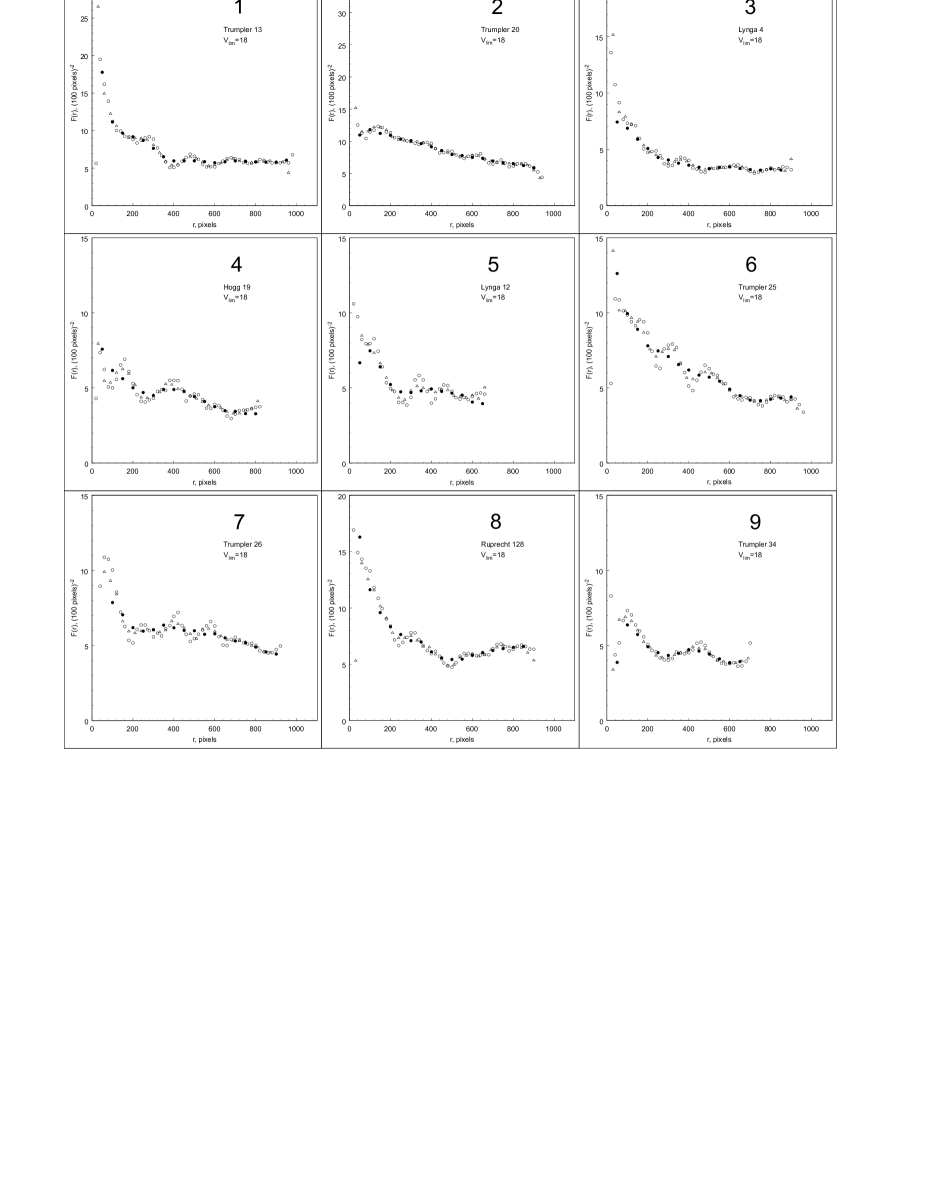
Figure 4: Radial Surface Density Profiles, F(r), for the nine fields under study. Different symbols indicate three different increments used to establish N(r): open circles correspond to 20 pixel (7.38^′′) steps, open triangles to 30 pixel (11.07^′′) steps, and filled circles to 50 pixel (18.45^′′) steps. See text for details

2 Previous investigations

In this Section we summarize previous results, if any, for the fields under investigation. In most cases we are referring to 2MASS archival data analysis. Each cluster is identified with its name and the number listed in Table 1.

1. Trumpler 13
Discovered by Trumpler (1930), this object was classified as a medium richness, $\sim 5\mbox{${}^{\prime}$}$ diameter, star cluster by van den Bergh & Hagen (1974). The only observational data for this object are those given in the 2MASS catalog and discussed by Bica & Bonatto (2005). These authors suggest that Trumpler 13 is an intermediate-age cluster ($\sim$ 300 Myr old), located at 2.5 kpc from the Sun in the third Galactic quadrant. We note that this cluster is in fact located in the fourth Galactic quadrant (see Table 1).

2. Trumpler 20
This cluster was also discovered by Trumpler (1930), and it is described as a rich open cluster, with a diameter of $\sim 7\mbox{${}^{\prime}$}$, by van den Bergh & Hagen (1974). The only study of Trumpler 20 that we are aware of is that by McSwain & Gies (2005), who provide shallow Stromgren photometry aimed at finding Be stars in open clusters. They suggest that this cluster is about 150 Myr old, and located at 2.5 kpc from the Sun. Their CMD (their Fig. 59) shows however a prominent clump, which attracted our attention and seems to indicate a much larger age. During the revision of this paper we came across to the first paper on this cluster by Platais et al. (2009), who suggest the cluster is indeed relatively old basing on optical photometry and Echelle spectroscopy. They derived a reddening E(B-V)=0.46, an age of 1.3 Gyr and a metallicity [Fe/H]=-0.11. The cluster is found to be located at 3.3 kpc from the Sun.

3. Lynga 4
This cluster is first mentioned in the search for open clusters by Lynga (1964). It has subsequently been investigated by Moffat & Vogt (1975), who do not find any indication for the existence of a cluster at the location of Lynga 4. Humphreys (1976) identified one supergiant star in the field of Lynga 4 (to which she assigns a distance of 4 kpc), but did not address the issue of the cluster reality. Recently, from 2MASS photometry, Bonatto & Bica (2007) infer that Lynga 4 is indeed a star cluster, of old age ($\sim$1 Gyr), but located at just 1.0 kpc from the Sun.

4. Hogg 19
No studies have been carried out in the field of Hogg 19 after its discovery by Hogg (1965).

5. Lynga 12
As Lynga 4, this cluster was first mentioned in Lynga (1964). The only observational data-set for this object is that given in the 2MASS catalog and discussed by Bica et al. (2006). They find that Lynga 12 is a real cluster, at the same distance as Lynga 4 (1.0 kpc), but with only half the age of the latter.

6. Trumpler 25
Discovered by Trumpler (1930), this object is classified as a medium richness, $\sim 6\mbox{${}^{\prime}$}$ diameter, cluster by van den Bergh & Hagen (1974). To the best of our knowledge, no other studies have been carried out of the field of this object.

7. Trumpler 26
This cluster was also discovered by Trumpler (1930). The only observational data-set for this cluster is that given in the 2MASS catalog, and discussed by Bonatto & Bica (2007). As was the case of Lynga 4 and Lynga 12, Trumpler 26 also lies at 1 kpc from the Sun. It is considered to be of intermediate age ($\sim$ 0.7 Gyr).

8. Ruprecht 128
First listed by Ruprecht (1966), this object was subsequently never studied until it was re-discovered by van den Bergh & Hagen (1974), and classified as a medium richness cluster with a diameter of $\sim$ 6 arcmin.

9. Trumpler 34
Discovered by Trumpler (1930). The only study of this cluster is that by McSwain & Gies (2005), who provide shallow Stromgren photometry aimed at finding Be stars in open clusters. They suggest that it is 100 Myr old, and located at 2 kpc from the Sun.

3 Star counts, cluster reality and cluster size

3.1 Surface Density Maps and Radial Surface Density Profiles

Surface Density Maps (SDM) and Radial Surface Density Profiles (RSDP) were constructed for all fields under investigation in order to determine each cluster’s reality and size. Example applications of this technique can be found in Prisinzano et al. (2001), and Pancino et al.(2003).

SDM were constructed using the kernel estimation method (see e.g. Silverman 1986), with a kernel half-width of 300 pixel (corresponding to 1.845^′), and a grid of 25-pixel cells. The large kernel half-width (HW) chosen is meant to diminish the effect of density fluctuations (and avoid, for example, numerous density peaks inside a cluster), and in order to detect the cluster centre clearly. Only stars brighter than $V$=18 mag were considered because the inclusion of faint stars usually has the negative effect of making the cluster disappear against the background. To avoid undersampling, we only made use of the 1450 $\times$ 1450 pixel ($\sim 9.6\mbox{${}^{\prime}$}\times 9.6\mbox{${}^{\prime}$}$) central region. The resulting SDMs are shown in Fig. 3, where the isodensity contour lines plotted are in units of (100 pixel)^-2.

New, rough coordinates for the clusters centres were obtained from the centre of symmetry of the inner (maximum) density contours. The new clusters centres coordinates are given in Table 4, and they are depicted by crosses in Fig. 3. It should be noted that the use of sophisticated methods for cluster centre determination do not make sense in this case, because the position of the cluster centre clearly depends on limiting magnitude, and on kernel half-width.

Following the procedure described in Seleznev (1994), RSDP, F(r), were obtained by differentiation of the polynomials fitted to the cumulative star counts function (the number of stars inside a circle of radius r), N(r). Third order polynomials were employed in all cases .

The resulting RSDP, for each field are shown in the Fig. 4. Different symbols indicate three different increments (steps) used to construct N(r): open circles correspond to 20 pixel (7.38^′′) steps, open triangles to 30 pixel (11.07^′′) steps, and filled circles to 50 pixel (18.45^′′) steps. F(r) is shown in units of (100 pixel)^-2, and only stars brighter than $V$=18 mag were considered, as was the case of the SDMs shown in Fig. 3.

Close inspection of Fig. 4 may draw the attention to the small values of F(r) at the cluster centres position in some cases. They are due to irregularities in the field in some cases caused by patchy extinction and/or field density fluctuations. Technically, the reason is that the cluster centres were determined from SDMs constructed with a large kernel half-width (300 pixel), whereas the RSDPs have been derived adopting smaller values for the kernel width. The smaller scale produces a fluctuating profile, and as a consequence low density values can be obtained at the centres when N(r) (and therefore F(r)) constructed using small increments.

3.2 Star counts

With the aim of obtaining field star decontaminated CMDs (see Sect. 5), the fields were divided into inner (cluster) and outer (comparison field) regions of equal area (see Fig. 3). Circular areas were used as inner regions, and, when possible, full rings were used as outer regions. When the cluster centre was found to be too close to the field boundary, ring sectors -with an area equal to that of the corresponding inner circles- were used as outer regions. In the case of fields 8 and 9, where there is more than one high density fluctuation, relatively small circular inner regions, containing only the cluster core, were selected. For these two fields, the comparison regions used were both ring sectors and circles, equal in area to the corresponding inner regions.

Due to the relatively small size of our fields we cannot use quantitative statistical methods for cluster size determination (Danilov et al. 1986, Danilov and Seleznev 1994); therefore we cannot prove that the inner regions completely contain the clusters. Furthermore, in some cases the cluster is larger than our FOV, therefore the inner region would only contain the cluster core, and, when using the outer regions for comparison, we would be subtracting stars both from the field and from the cluster halo. This is not a major problem because we are mostly interested in the CMD’s main features, which would still be visible (note that in these cases the inner region is much denser than the outer region). Besides, in these regions of the Milky Way extinction is highly variable, and selecting comparison field too far apart (see Bonatto and Bica 2007) introduces unpredictable effects in star counts due to reddening variations which are difficult to properly manage.

The parameters defining the regions selected in each field are presented in Table 4. The first and second columns give the clusters labels and names, respectively, in agreement with Table 1. Columns (3) and (4) provide the new cluster centres in pixels, and columns (5) and (6) the newly determined coordinates, respectively. Columns (7,8) give the radius of the inner (cluster) regions in pixels and arcmin, and column (9) the outer radius of the outer (comparison) region, in pixels, respectively. Columns (10) and (11) list the starting and ending position angles, $\phi$, for ring sectors in degrees. These position angles are measured counterclockwise from the south (positive Y direction). Values of 0^o or 360^o imply that a full ring has been used. Finally, columns (12) and (13) give the centres of the circular comparison regions used in the case of fields 8 and 9, as explained above.

Table 4: Cluster centres and parameters defining the inner (cluster) and outer (comparison) regions in each field. RA and Dec are the newly determined coordinates of the clusters centres, obtained from the centre of symmetry of the inner (maximum) density contours.

Label	Name	$X_{C}$	$Y_{C}$	$RA$	$Dec$	$r_{1}$	$r_{1}$	$r_{0}$	$\phi_{1}$	$\phi_{2}$	$X^{{}^{\prime}}_{C}$	$Y^{{}^{\prime}}_{C}$
		pixel	pixel	$hh:mm:ss$	o : ′ : ′′	pixel	${\prime}$	pixel	deg.	deg.	pixel	pixel
1	Trumpler 13	1040	1048	10:23:48	-60:08:09	709	4.7	1002.7	0	360
2	Trumpler 20	1094	1059	12:39:32	-60:37:36	675	4.5	954.6	0	360
3	Lynga 4	1110	937	15:33:17	-55:13:28	655.5	4.3	927	0	360
4	Hogg 19	842	1028	16:28:55	-49:06:02	669	4.4	1021.9	315	225
5	Lynga 12	1010	1362	16:46:04	-50:48:03	657	4.3	1009	48	313
6	Trumpler 25	1067	1059	17:24:28	-39:01:13	689.4	4.6	975	0	360
7	Trumpler 26	1009	1106	17:28:33	-29:30:31	390	2.6	675.5	290	110	387	1660
											1626	1602
											1640	400
											675	400
8	Ruprecht 128	1028	1124	17:44:18	-34:53:37	439	2.9	760.4	90	270	1598	450
											450	450
9	Trumpler 34	1114	1324	18:39:46	-08:26:14	609	4.0	930.2	45	315

3.3 Results from the SDM and RSDP analysis

1. Trumpler 13
This cluster is clearly elongated in the South-North direction and has a tail in the South-West direction. It is not seen in the RSDP (Fig. 4) because this profile is a spherically symmetric approximation which includes the low-density regions to the East and West. Trumpler 13 shows a clear transition zone (following terminology of Danilov and Seleznev (1989); also see Seleznev (1994)), from 160 to 400 pixels. Only the outer boundary of this transition zone is seen in the RSDP; the cluster’s halo is not visible due to field star fluctuations. Nevertheless, our cluster (inner) region contains nearly the entire cluster. Taking into account the tail, we estimate that the cluster’s radius is larger than 400 pixels (2.6^′).

2. Trumpler 20
This is a large cluster covering nearly the entire field, as clearly seen in both its SDM and RSDP. The RSDP indicates that the cluster’s radius is larger than 950 pixels (5.8^′). The cluster’s core is clearly elongated in South-East/North-West direction, and it is asymmetric. The cluster region contains only the dense core of Trumpler 20 (see Tables 4 and 5).

3. Lynga 4
This object looks like a small cluster with symmetric core, but with and asymmetric halo elongated to the North-East. From its SDM and RSDP we estimate that the lower limit of the cluster’s radius is 500 pixels (3.1^′), and 480 pixels (3 ^′), respectively.
The cluster is fully contained inside our cluster region.

4. Hogg 19
This cluster exhibits a very irregular and asymmetric structure. The RSDP yields a radius estimate of 680 pixels (4.2^′), or possibly larger, which is slightly more than the inner region we selected. It is difficult to estimate its radius from the SDM, but its SDM seems to indicate a larger cluster size.

5. Lynga 12
This over-density has highly asymmetric structure. It is difficult to estimate its radius; the SDM suggests that it might be larger than 700 pixels (4.3^′), and the RSDP indicates that it is larger than 650 pixels (4^′). The complicated structure seen in the SDM may be the result of strong irregularities in the extinction distribution, giving origin in turn to a cluster-like aspect.

6. Trumpler 25
It is a well-defined cluster with an asymmetric form elongated in the South-North direction. The SDM does not show the cluster’s boundaries, and the RSDP indicates a cluster radius of more than 960 pixels (5.9^′). Our cluster region contains all of the cluster core and a large part of its intermediate zone.

7. Trumpler 26
The density maximum considered as the cluster centre seems to be part of a larger structure. It is not clear if this is a physically connected structure, or a projection effect. It is very difficult to estimate the cluster radius from the SDM, because it does not have a cluster-like structure. The RSDP indicates a small core, and then a gradual decrease of the density outwards. If it is a true cluster, then its radius is more than 900 pixels (5,5^′), and it would include both the eastern and western density maxima seen in the SDM.

8. Ruprecht 128
This cluster looks like a small fluctuation near a very dense field most probably related to the Galactic bulge. It is very difficult to estimate the cluster radius from the SDM because it is overlapped with the density gradient caused by the dense field towards the South-East. The RSDP gives radius estimate of about 480 pixels (3^′), in which case our cluster region would include nearly all the cluster.

9. Trumpler 34
The SDM reveals a very irregular and asymmetric structure. The probable cluster centre is offset with respect to the centre of the field, which makes it difficult to estimate the cluster radius from the SDM. The RSDP indicates a cluster radius larger than 600 pixels (3.7^′), while density map suggests an even larger size. We consider this a dubious case, and will turn back to it in the next Section.

In Table 5 we summarize our radius estimates obtained from the SDM and RSDP analysis for the 11 clusters studied here.

Table 5: Estimates of the cluster’s radii, R, from the SDM and RSDP analysis. A question mark in the last column indicates a dubious case.

Label	Name	$R$	$R$	$Note$
		pixels	′
1	Trumpler 13	$\geq$ 400	$\geq$ 2.6
2	Trumpler 20	$>$ 950	$>$ 5.8
3	Lynga 4	$\geq$ 500	$\geq$ 3.1
4	Hogg 19	$>$ 680	$>$ 4.2
5	Lynga 12	$\geq$ 700	$\geq$ 4.3	$?$
6	Trumpler 25	$>$ 960	$>$ 5.9
7	Trumpler 26	$>$ 900	$>$ 5.5	$?$
8	Ruprecht 128	$\geq$ 480	$\geq$ 3.0
9	Trumpler 34	$\geq$ 600	$\geq$ 3.7	$?$

Table 6: Parameters used to analyze 2MASS star counts and revised cluster centres.

Label	Name	HW	Grid	Jlim	(J-H)lim	RAcentre	DECcentre
		′	′	mag	mag	$hh:mm:ss$	o : ′ : ′′
1	Trumpler 13	3.0	0.5	16.0	0.6	10:23:49	-60:08:12
2	Trumpler 20	5.0	0.5	16.0	0.7	12:39:34	-60:38:42
3	Lynga 4	5.0	0.5	12.0	0.8	15:33:23	-55:14:06
4	Hogg 19	5.0	0.5	16.0		16:29:03	-49:05:24
5	Lynga 12	5.0	0.5	12.0	0.7	16:46:06	-50:45:30
6	Trumpler 25	5.0	0.5	16.0	0.7	17:24:30	-39:00:30
7	Trumpler 26	5.0	0.5	16.0	0.7	17:28:35	-29:28:54
8	Ruprecht 128	3.0	0.5	16.0	0.7	17:44:17	-34:53:06
9	Trumpler 34	5.0	0.5	14.0	0.7	18:39:39	-08:25:48

Figure 5: Q-based cluster stars selection for Trumpler 20. The solid line is a reference observational relation. The size of the dots are proportional to the magnitude errors. See text for details.

4 Results from the 2MASS archival data analysis: star counts and surface density profiles in a larger area

The results of previous Section contain two basic limitations. Firstly, the star clusters have larger sizes than the area covered by the detector under use in many cases. Second, in the optical it is more difficult to account for reddening variations across the clusters’ field, especially toward the dense inner Galaxy, where we are looking at.

To cope with these difficulties, we made use of photometry from the 2MASS archive, and re-performed the star counts analysis in a larger field of view, to determine in more solid way clusters’ reality and radii.

4.1 Cluster members’ selection

In details, we extracted from 2MASS JHK_s photometry for stars inside a box 60 arcmin on a size, and adopted the same technique as in the previous section to perform star counts, and build up $J$ density maps and clusters’ radial surface density profiles.

The parameters used and the new cluster centres’ coordinated are reported in Table 6. The adopted magnitude limits have been chosen to decrease the noise in star counts and to highlight the cluster more clearly. Together with a cut-off in magnitude, we also use a color (J-H) cut-off in the range 0.6$-$0.8 mag, depending on the cluster, to decrease the amount of expected red field stars.
An additional, more stringent, criterion has been applied to filter out interlopers, as follows. Firstly, we derived an estimate of the reddening in the cluster region using the Q vs (J-H) diagram, being Q defined as:

$$Q_{JHK}=(J-H)-\frac{E_{J-H}}{E_{H-K}}\times(H-K),$$ (3)

following Straizys (1992).
From Bessell and Brett (1988)we have then:

$$E_{J-H}=0.37\times E_{B-V}$$ (4)

$$E_{H-K}=0.19\times E_{B-V},$$ (5)

and, hence,

$$\frac{E_{J-H}}{E_{H-K}}=0.37/0.19\simeq 1.95.$$ (6)

Therefore, we are making use of the following expressions:

$$Q_{JHK}=(J-H)-1.95\times(H-K),$$ (7)

and

$$K=K_{s}+0.044$$ (8)

from Sarajedini (2004).
In details, we started selecting stars in a region close to the cluster peak (tipycally 5 arcmin), to alleviate field star contamination. This Q-based selection basically picks up stars having compatible reddening, and therefore probable clusters’ members. This, in turn, results in a better contrast between cluster and field, and in a more robust estimate of cluster size and reality. The method is illustrated in Fig. 5 for the case of Trumpler 20, one of the most prominent cluster of our sample. In the figure the size of the dots are proportional to the errors from 2MASS magnitudes, and the solid line is the above relation calibrated by us with stars from 200 nearby well studied open clusters. By shifting horizontally this line we can get an estimate of the cluster reddening, which for Trumpler 20 turned out to be E(J-H) = 0.08. Then, we extract from the entire sample all the stars (probable members) having reddening within 0.15 mag from the mean Trumpler 20 reddening.

We found this procedure effective for Trumpler 13, Trumpler 20, Hogg 19, Trumpler 25 and Ruprecht 128, for which we estimated E(J-H) = 0.03, 0.08, 0.16, 0.14, and 0.20, respectively. In the other 4 cases we could not come out with a reliable estimate, due to the heavy contamination and noise of the 2MASS plot. For these latter 4 cases, we used as a first E(J-H) guesses estimates from literature data. Namely, we took E(J-H) from Bonatto & Bica (2007) for Lynga 4 (0.25) and Trumpler 26 (0.12), from Bonatto et al. (2006) for Lynga 12 (0,08), and from McSwain & Gies (2005) for Trumpler 34 (0.20). Adopting these values, we used the Q versus (J-H) diagram to select stars along the Zero Age Main Sequence (ZAMS), as for Trumpler 20.  These final samples have been used to perform star counts.

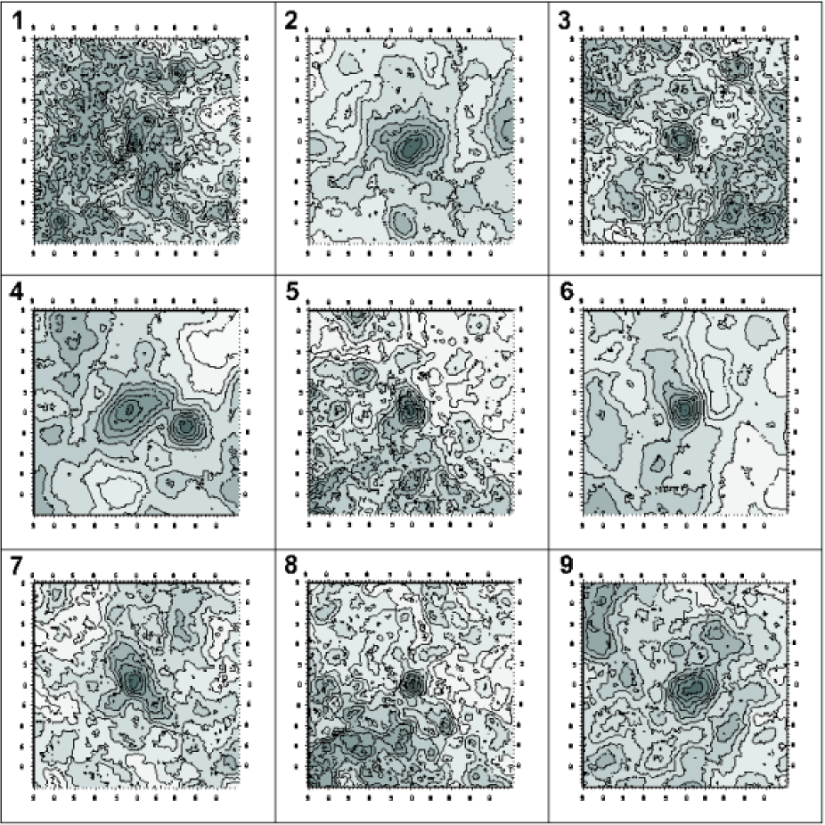
Figure 6: Surface Density Maps from 2MASS for the nine fields under study. Numbers in the upper-left corners indicate the cluster label, in agreement with Table 1. They have been constructed using kernel half-widths, magnitude limits in J and grids as in Table 6. In panel 4, the overdensity close to Hogg 19 is the open cluster NGC 6134

4.2 Results and comparison with the analysis of the optical data

We used exactly the same method as for the optical data to perform star counts and derive radial surface density profiles. Results are shown in Figs.  6 and 7, and summarized in Tables  6 and 7.
Table 6 lists the values adopted for the size of the cell grid and half-width kernel, together with the magnitude and color limits. The first result is a new determinations of the cluster centers (see columns 7 and 8 in the same table). By comparing these new coordinates with the ones derived from optical star counts, we find that there is a general agreement (within less than an arcmin both in RA and DEC) between the cluster centres in the optical and in the infra-red, except for Lynga 12, for which the centre DEC differs by 2.5 arcmin.

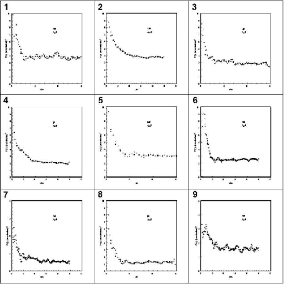
Figure 7: Radial Surface Density Profiles, F(r), for the nine fields under study as derived from 2MASS. Here filled circles refer to 1 arcmin, open circlesto 0.5 arcmin, and crosses to 0.25 arcmin steps.

Table 7: Estimates of the cluster’s radii, R, from the SDM and RSDP analysis.

Label	Name	Radius	Core radius
		′	′
1	Trumpler 13	3.5	2.5
2	Trumpler 20	17.0	5.0
3	Lynga 4	7.5	2.0
4	Hogg 19	14.0	3.0
5	Lynga 12	8.0	4.0
6	Trumpler 25	7.0	4.5
7	Trumpler 26	13.0	4.0
8	Ruprecht 128	5.0	2.0
9	Trumpler 34	13.0	5.0

In Table 7 we present new estimates of the clusters’ radii (column 3) and core radii (column 4). Notice, for the sake of clarity, that these core radii are not the King core radii, since we are not fitting any King model (King 1962). While the clusters’ radii we find with 2MASS are, as expected, larger than the optical estimates, the core radii we estimate are on the average comparable with the adopted cluster area in the optical anlysis (see column 8 -r1- in Table 4).
Most cluster stars are presumed to be located inside the core radius, while outside the core radius still there are cluster stars, but heavily mixed with the field. Basing on that, we are going to use the core radii from Table 5 to define the clusters’ region, and the regions depicted in Fig. 3 as field regions, to clean in a statistical way the cluster regions and derive field stars decontaminated CMDs in the following Section.

5 Color Magnitude Diagrams and Cluster Fundamental Parameters

In this Section we make use of the results obtained in previous Sections to construct field star decontaminated (”clean”) CMDs, and to derive new estimates of the clusters fundamental parameters.

5.1 Methodology

To alleviate the high contamination from Galactic disk stars, we employ the same statistical subtraction technique used in Carraro & Costa (2007) and in Baume et al. (2007), which was adapted from Gallart et al. (2003).

Briefly, for all objects in the comparison regions we search for the most similar star, in color and magnitude, in the cluster region, and remove it from the CMD of the cluster. Matching is done by means of a search ellipse, whose semi-major and semi-minor axis depend on the photometric errors (see Fig. 2), and their ratio is taken as 5. If a field star has a counterpart in the cluster area within this ellipse, the counterpart is removed from the cluster CMD.
It should be noted that the procedure also takes into account the completeness level of the photometry (see Sect. 2). The cluster region and the comparison region were selected as explained in Sect. 4.2.

Having realized the statistical subtraction, the clean CMDs are compared with theoretical isochrones from the Padova suite of models (Girardi et al. 2000a). Because we are basically interested in deriving estimates of the cluster fundamental parameters, which in most cases are first estimates, adopting the general extinction law is a reasonable assumption. In this case, the total to selective absorption ratio, $R_{V}=\frac{A_{V}}{E(B-V)}$, is equal to 3.1. As a consequence one can adopt the relation $E(V-I)$ = 1.244 $\times E(B-V)$ to derive $E(B-V)$. Since we are exploring a region inside the solar ring, adopting a solar metallicity (Z=0.019) in the models seems to be a reasonable choice. The distance of the Sun from the Galactic centre was taken as 8.5 kpc, to be homogeneous with our previous studies.

To assess the reliability of the above procedure, and strenghen our findings, we make also use of the 2MASS photometry, and build up infrared CMDs. We refer to the 2MASS star counts performed in the previous section, and extract JHK photometry for all the stars inside the core radius (see Table 7) and by means of the Q-paramter previouslly described (see Sec. 5). This photometry is then analyzed and compared to the same set of theoretical isochrones. We adopt E(J-H) = 0.29 $\times$ E(V-I) and E(H-K) =0.19$\times$ E(B-V) from Bessel & Brett (1988).

5.2 Cluster Fundamental Parameters

The results of our analysis are summarized in Table 8, where for each cluster we list the age, reddening ($E(V-I)$), apparent distance modulus (m-M)_V, distance from the Sun ($d_{\odot}$) and location in the Galactic disk ($X_{GC}$, $Y_{GC}$, $Z_{GC}$, $d_{GC}$). The uncertainties for the age, reddening and apparent distance modulus given in Table 6 were derived by adopting different age isochrones (for the sake of the clarity not shown in the CMDs presented in the next Section), and moving the best fit isochrones back and forth in the horizontal and vertical direction to adjust reddening and distance modulus.
In these series of Figs.  8 to 16 we show in the bottom panels, from left to right, VI photometry for cluster (left panel) and field (middle panel), as selected in Fig. 3 and Table 4, and the decontaminated CMD (right panel), together with the best fit isochrone.

This same isochrone is used in the upper panels, where, from the left to the right we show JHK photometry for the cluster field (left panel, see Table 7), for the stars selected according to the Q-parameter (middle panel, see Section 5) and, finally, the CMD with these latter stars, where an isochrone fit is provided for the same set of parameters used in the optical CMD.

5.3 Color Magnitude Diagrams

1. Trumpler 13
See Fig. 8. This object is located in the fourth Galactic quadrant just before the tangent to the Carina branch of the Carina-Sagittarius spiral arm, and for this reason we do not expect important contamination from spiral features. The CMD of the cluster region differs from that of the comparison region in the upper part of the Main Sequence (MS). A blue MS, with a turn-off (TO) at $V\approx 15.5$, is clearly visible in the cluster CMD, but only marginally present in the comparison CMD, and survives the cleaning process. The blue solar metallicity isochrone plotted in the right panels is for the fundamental parameters listed in Table 8. Notice the consistency between the optical and IR results. Apart from the location (in the fourth and not in the third quadrant) we basically agree with Bica and Bonatto (2005) results.

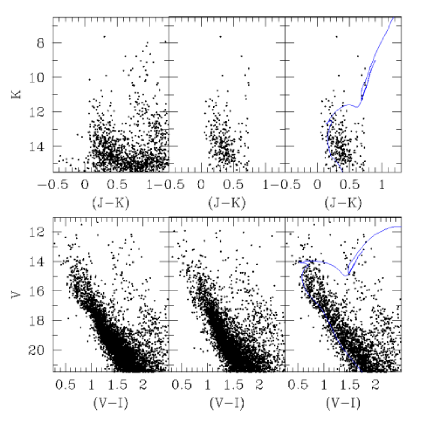
Figure 8: CMDs for Trumpler 13. Bottom panels. In the left panel we show the inner cluster region CMD, in the middle panel the outer comparison/field region CMD, and in the right panel the corresponding clean CMD (3021 stars). Top panels. In the left panel we show the JHK CMD for the star within the core radius, in the middle panel the CMD for the same stars but after a selection according to the Q-parameter. Finally, in the right panels these same latter stars are used to perform an isochrone fit for set of fundamental parameters listed in Table 8. The same isochrone is used in the lower right panel.

2. Trumpler 20
See Fig. 9. Although this cluster is located about 2^o above the Galactic plane, some contamination from young stars of the Carina arm is still visible in the clean CMD. This sequence was erroneously attributed to Trumpler 20 by McSwain and Gies (2005), but, by adjusting a Schmidt-Kaler (1982) empirical ZAMS -hereafter empirical ZAMS- (red line), it can be inferred that it corresponds to a sector of the Carina arm at a distance of about 2 kpc (see also Platais et al. 2009, who highlighted the same problem).
Trumpler 20 is in fact a much older cluster, as indicated by the conspicuous clump of red giant branch (RGB) stars seen both in the cluster region CMD, and in the clean CMD. There is no doubt that Trumpler 20 is an intermediate age cluster, very much resembling NGC 7789 (Gim et al 1995). It is somewhat surprising that this fact was not noticed before, and certainly deserves further investigation. The blue solar metallicity isochrone plotted is consistent with the fundamental parameters listed in Table 8 which, in turn, nicely agree with the recent study by Platais et al.(2009). Notice the consistency between the optical and IR results.

An interesting feature of Trumpler 20 CMD is the presence of a double red clump, which strenghten its similarity to NGC 7789 and other intermediate age star clusters, like NGC 5822 and NGC 2660 (Girardi et al. 2000b). Such occurence is not limited to star clusters in the Milky Way, but is also present in the Magellanic Clouds clusters (Girardi et al. 2009).

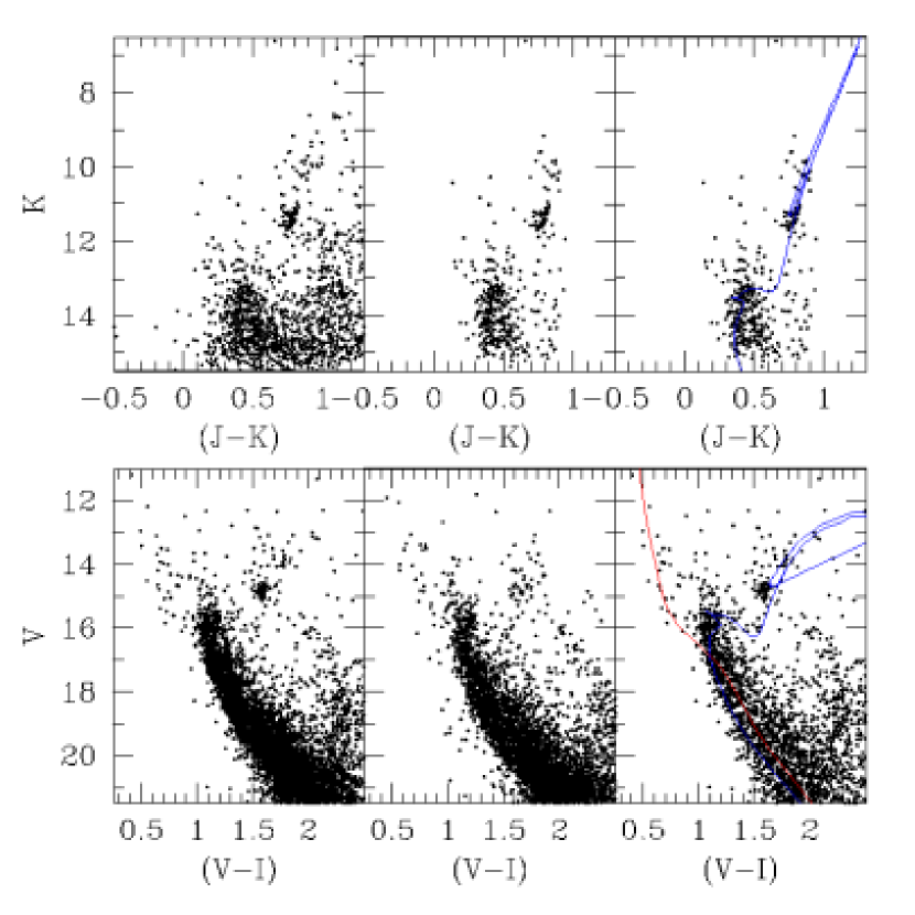
Figure 9: Same as Fig. 8, but for Trumpler 20. The clean optical CMD contains 3250 stars.The blue solar metallicity isochrone is consistent with the fundamental parameters listed in Table 8, whereas the red line is an empirical ZAMS.

3. Lynga 4
See Fig. 10. This cluster is clearly visible from IR photometry, and its basic parameters have determined by fitting the blue isochrones in the upper-right panel. This fit implies an age of 300 million years, a reddening E(V-I)=1.9 and a distance of 1.1 kpc. The age we find is significantly lower than Bonatto & Bica (2007) estimate.
Due to the extreme absorption, in the optical CMD (botton panels in Fig. 10) the cluster looks very faint and its MS is mixed with the general Galactic field stars. However, the bifurcation we see at V$\sim$ 18.0 and (V-I) $\sim$ 1.2, together with the bunch of red stars at 16 $\leq V\leq 17$ (probable giants), make us confindent about the cluster identification.

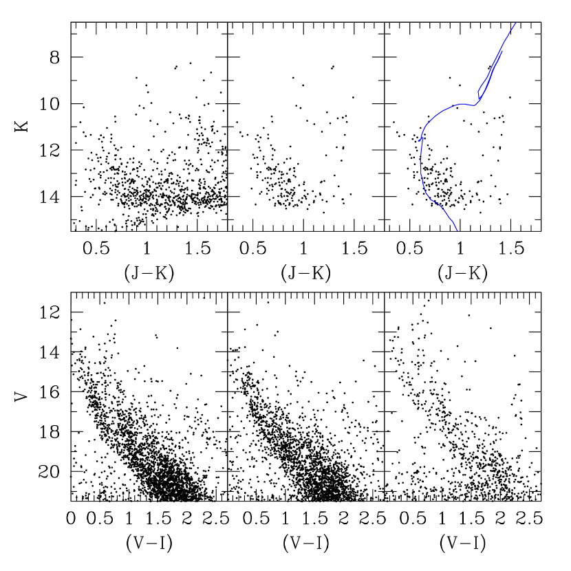
Figure 10: Same as Fig. 8, for Lynga 4. The blue solar metallicity isochrone is consistent with the fundamental parameters listed in Table 8. We could not see any cluster in the optical data, and therefore no isochrone fit is shown. The clean optical CMD contains 3185 stars. See text for details.

4. Hogg 19
See Fig. 11. This field is located quite low in the Galactic plane (see Table 1), in the direction of the Carina-Sagittarius spiral arm. FIRB reddening (Schlegel et al. 1998) in the direction of Hogg 19, amounts to $\approx$ 21 mag. Three sequences of stars are seen in Fig. 11. 1: a sequence of bright young stars, present both in the cluster region and in the comparison region, which we interpret as a young diffuse population from the spiral arm; 2: a population of red giant stars, which is significantly larger in the cluster region than in the field; 3: a fainter thick main sequence, which is much thicker in the cluster region than in the field. This latter sequence survives in the clean CMD and we relate it to the group of giants stars that survive as well. This indicates the presence of an old age star cluster in the field. We see a Turn Off point at V$\sim$ 18.0 mag and (V-I ) $\sim$ 1.4. The cluster (Hogg 19) is located in front of the spiral arm. An empirical ZAMS fit to the young population (red line) yields a distance of 2.4$\pm$0.3 kpc, for a reddening of 0.9$\pm$0.2 mag. The blue solar metallicity isochrone plotted is consistent with the fundamental parameters listed in Table 8. An age of about 2 Gyrs is derived both from the optical and IR data.

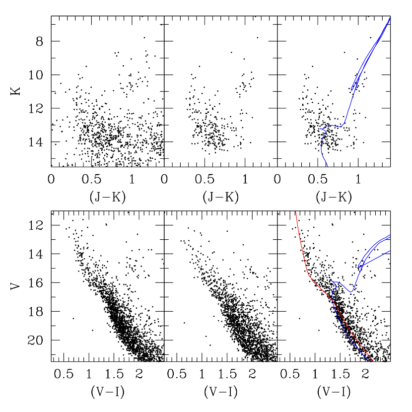
Figure 11: Same as Fig. 8, for Hogg 19. The blue solar metallicity isochrone is consistent with the fundamental parameters listed in Table 8, whereas the red line is an empirical ZAMS drawn to highlight the presence of a strong field contamination caused by the fore-ground Carina arm. The clean optical CMD contains 1409 stars. See text for details.

5. Lynga 12
See Fig. 12. The analysis of 2MASS data reveals that Lynga 12 is a young cluster, suffering heavy extinction. This is confirmed by our optical data. The fit in the lower right panel of Fig. 12 is with a ZAMS, shifted by E(V-I) = 1.00 and (m-M) = 13.8, which implies a distance of 1.8 kpc. This young aggregate is therefore located inside the Carina-Sagittarius spiral arm. It is quite difficult to estimate the age of the cluster. While in the optical there is no clear indication of evolved stars, IR data seems to indicate an age around 200 Myr (the red isochrone super-posed in the two right panels).

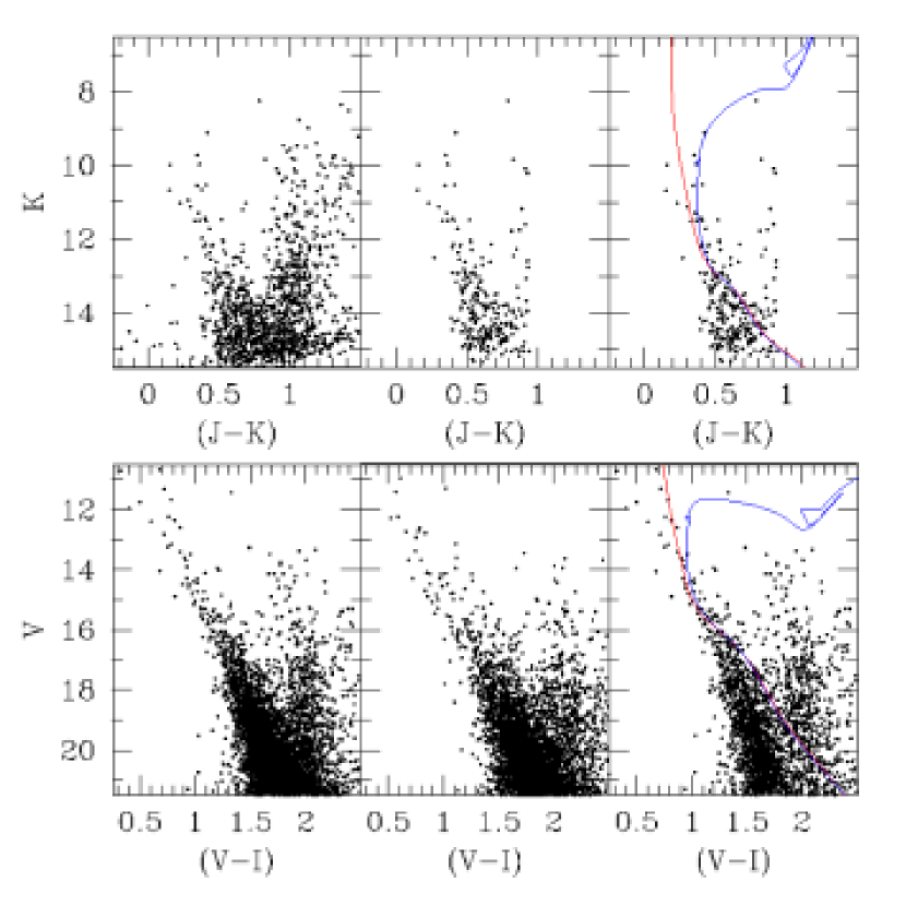
Figure 12: Same as Fig. 8, for Lynga 12.The blue isochrone is consistent with the fundamental parameters listed in Table 8. The clean optical CMD contains 2894 stars. See text for more details.

6. Trumpler 25
See Fig. 13. In the cluster region CMD we recognize a bifurcation in the MS at $V\approx 15.5$, together with an excess of giant stars in comparison to the control field CMD. We tentatively interpret the bluer MS as a diffuse stellar population in the Carina-Sagittarius arm, while the red MS is the star cluster Trumpler 25. The isochrone fitted (blue line) indicates that this latter is about 0.5 Gyr old, and located at about 2 kpc from the Sun. Notice the consistency between optical and IR data. (see Table 8).

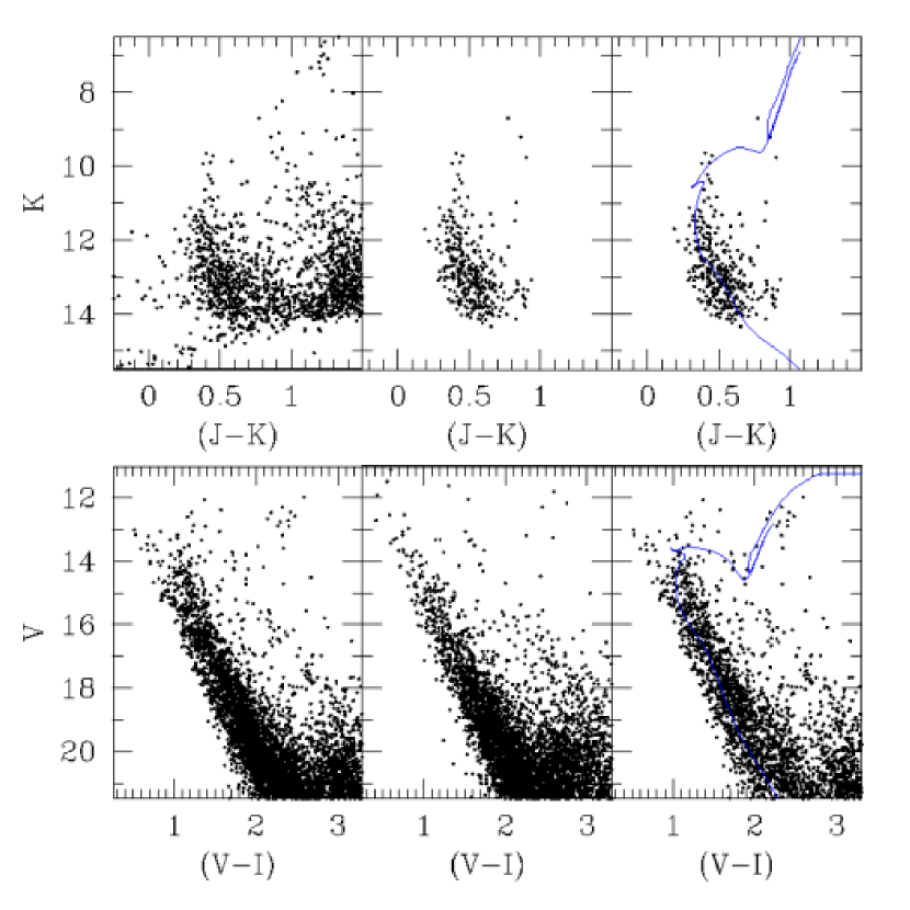
Figure 13: Same as Fig. 8, for Trumpler 25. The blue isochrone is consistent with the fundamental parameters listed in Table 8. The clean optical CMD contains 3030 stars. See text for details.

7. Trumpler 26
See Fig. 14. For this cluster we defined two comparison regions (see Fig. 3). We do not find any difference by adopting one or the other. This object lies in a direction very close to the line of sight to the Galactic bulge, which also intersects the Carina-Sagittarius arm. An examination of Fig. 14 indeed shows a diffuse young stellar population. Both the IR and optical CMDs provide us with a $\sim$ 300 Myr poorly populated star cluster. The empirical ZAMS fitted (blue line) indicates a distance of about 1.22 kpc and a reddening E(V-I) = 0.5 mag.

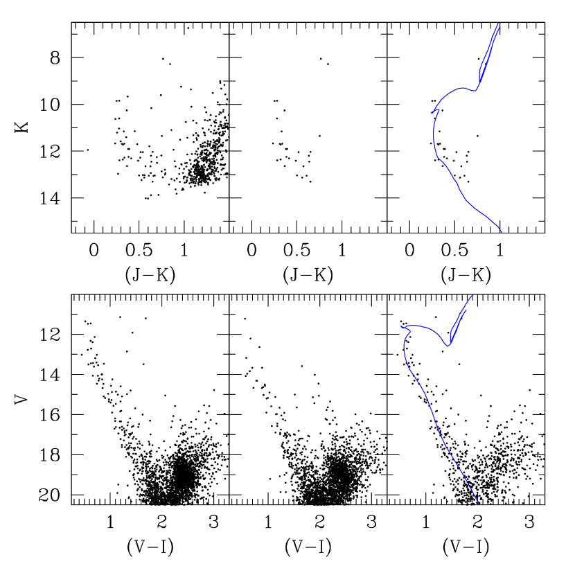
Figure 14: Same as Fig. 8, for Trumpler 26. The blue isochrone is consistent with the fundamental parameters listed in Table 8. The clean optical CMD contains 878 stars. See text for more details.

Table 8: Derived fundamental parameters of the clusters under investigation.

Label	Name	$Age$	$E(V-I)$	$(m-M)_{V}$	$d_{\odot}$	$X_{GC}$	$Y_{GC}$	$Z_{GC}$	$d_{GC}$
		Gyr	mag	mag	kpc	kpc	kpc	kpc	kpc
1	Trumpler 13	0.4$\pm$0.1	0.45$\pm$0.10	13.5$\pm$0.2	2.9	7.8	-2.8	-0.1	8.3
2	Trumpler 20	1.5$\pm$0.3	0.60$\pm$0.10	13.9$\pm$0.2	3.0	6.9	-2.5	0.1	7.3
3	Lynga 4	0.3$\pm$0.1	1.90$\pm$0.30	12.2$\pm$0.2	1.1	5.3	-0.6	0.0	7.6
4	Hogg 19	2.5$\pm$0.3	0.80$\pm$0.10	14.0$\pm$0.2	2.6	6.2	-1.0	0.0	6.7
5	Lynga 12	0.2$\pm$0.1	1.00$\pm$0.10	13.8$\pm$0.2	1.8	6.8	-0.7	-0.1	6.9
6	Trumpler 25	0.5$\pm$0.1	0.90$\pm$0.10	13.8$\pm$0.2	2.0	6.6	-0.7	0.1	6.6
7	Trumpler 26	0.3$\pm$0.1	0.50$\pm$0.10	11.7$\pm$0.2	1.2	7.3	-0.0	0.0	7.3
8	Ruprecht 128	0.8$\pm$0.1	1.00$\pm$0.20	13.5$\pm$0.2	1.6	6.9	-0.1	-0.1	6.9
9	Trumpler 34	0.2$\pm$0.1	1.00$\pm$0.10	12.9$\pm$0.2	1.2	7.5	0.5	-0.0	7.5

8. Ruprecht 128
See Fig. 15. The situation is similar to that of Trumpler 25. A well defined MS, with a clear TO, typical of intermediate-age open clusters is seen, together with a few young stars close to a ZAMS. The isochrone fitted (blue line) indicates an age around 1 Gyr and a heliocentric distance of 1.6 kpc, for a reddening of about 1 mag (see Table 8). The optical findings are corroborated by the 2MASS analysis.

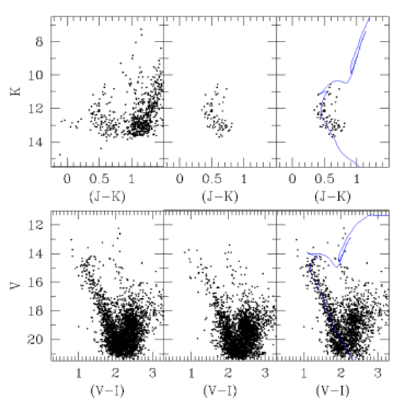
Figure 15: Same as Fig. 8, for Ruprecht 128. The blue isochrone is consistent with the fundamental parameters listed in Table 8. The clean optical CMD contains 1994 stars. See text for details.

9. Trumpler 34
See Fig. 16. This cluster is the loosest of the sample, and its density profile shows it stands weakly above the field and has a hole right in the centre. The CMD in the IR is quite broad in color, and is is difficult to see a clear sequence. Still, we performed some fitting using the parameters listed in Table 8. The fit is shown by means of the blue isochrone (right panels of Fig. 16). The cluster turns out to be relatively young, confirming McSwain & Gies (2005) suggestions.

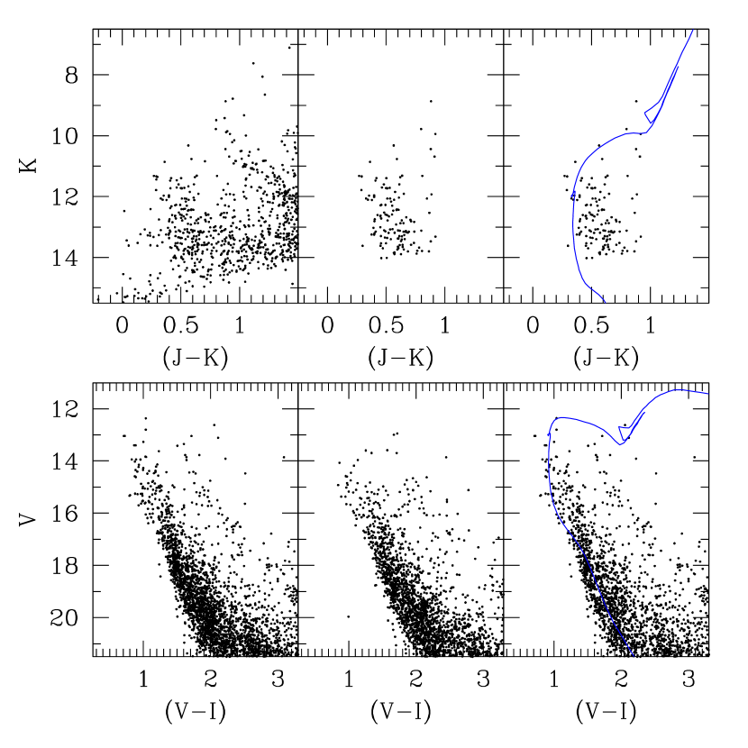
Figure 16: Same as Fig. 8, for Trumpler 34. The blue isochrone is drawn according to literature parameters, but we do not consider Trumpler 34 as physical group. The clean optical CMD contains 2184 stars. See text for more details.

6 Conclusions

We have presented homogeneous $V,I$ CCD photometry in the field of nine Galactic open clusters, obtained with the purpose of estimating, in many cases for the first time, their fundamental parameters. In most cases, this is the first CCD study in the cluster region.

We have performed a star count analysis of these fields to assess the clusters’ reality as over-densities of stars with respect to the field, and to estimate their radii. By means of comparison fields, and applying a statistical subtraction procedure, we have constructed field star decontaminated CMDs for these clusters. We complemented this data-set with photometry from 2MASS archive to test and strenghten our findings.

The analysis of the optical and IR CMDs, together with the results from the star counts, allowed us to determine estimates star clusters’ basic parameters.

Our finding can be summarized as follows:

$\bullet$ all clusters are found to be real, and of intermediate or old age;

$\bullet$ Hogg 19 is the oldest cluster of the sample, with an age around 2.5 Gyr; the existence of such an old cluster in a hostile environment as the inner Galaxy is puzzling;

$\bullet$ Lynga 4 is the most heavily reddened cluster in the sample, and we could detect it only in the IR;

$\bullet$ Trumpler 20 has been found to be quite an interesting cluster, much similar to NGC 7789. The most interesting result is the presence of a double red clump, which deserves further investigation.

This investigation emphasizes the difficulty to study the inner regions of the Galaxy in the mere optical domain. We show, however, that the combination of star counts and CMDs in the optical and IR, with common knowledge of the spiral structure of our galaxy, is quite an effective strategy to distinguish real star clusters from over-densities produced by the patchy distribution of dust, gas and stars in spiral arms.

Present and future wide area surveys in the IR, conducted by UKIDSS (Lawrence et al. 2007) and VISTA (McPherson et al. 2004) consortia, will certainly provide more suitable data to discover and study new star clusters in the inner Galaxy.

References

- Baume et al. [2007] Baume G., Carraro G., Costa E., Mendez R.A., Girardi L., 2007, MNRAS 375, 1077
- Baume et al. [2009] Baume G., Carraro G., Al Momany, Y., MNRAS, submitted
- van den Bergh and Hagen [1974] van den Bergh S., Hagen G.L., 1974, AJ 80, 11
- Bessell and Brett [1988] Bessell., M.S., Brett, J.M., 1988, PASO 100, 1134
- Bica and Bonatto [2005] Bica E., Bonatto C., 2005 A&A, 443, 465
- Bica et al. [2006] Bica E., Bonatto C., Blumberg G. 2006 A&A, 460, 83
- Bonatto and Bica [2007] Bonatto C., Bica E., 2007 MNRAS, 377, 1301
- [8] Carraro G., Méndez R.A., Costa E., 2005, MNRAS 356, 647
- [9] Carraro G., Janes K.A., Eastman J.D., 2005, MNRAS 364, 179
- Carraro et al. [2006] Carraro G., Janes K.A., Costa E., Méndez R.A., 2006, MNRAS 368, 1078
- Carraro and Costa [2007] Carraro G., Costa E., 2007, A&A, 464, 573
- Carraro and Costa [2009] Carraro G., Costa E., 2009, A&A, 493, 71
- Danilov et al. [1985] Danilov V.M., Matkin N.V., Pylskaya O.P., 1985, Soviet Astronomy, 29, 621
- Danilov and Seleznev [1989] Danilov V.M., Seleznev A.F., 1989, ATsir,1538, 9
- Danilov and Seleznev [1994] Danilov V.M., Seleznev A.F., 1994, A&AT, 6, 85
- Dias et al. [2002] Dias W.S., Alessi B.S., Moitinho A., Lépine J.R.D., 2002, A&A 389, 871
- Gallart et al. [2003] Gallart C., Zoccali M., Bertelli G., Chiosi C., Demarque P., Girardi L., Nasi E., Woo J-H, Yi S., 2003, AJ 125, 742
- Gim et al. [1998] Gim M., Vandenberg D.A., Stetson P.B., Hesser J.E, Zurek D.R., 1998, PASP 110, 1318
- [19] Girardi L., Bressan A., Bertelli G., Chiosi C. 2000a, A&AS, 114, 371
- [20] Girardi L., Mermilliod, J.-C., Carraro, G., 2000b, A&A 354, 892
- Girardi et al. [2009] Girardi L., Rubele, S., Kerber, L., 2009, MNRAS 394, L74
- Hogg [1965] Hogg A.R., 1965, PASP 77, 440
- Humphreys [1976] Humphreys R.M., 1976, PASP 88, 647
- King [1962] King, I., 1962, AJ 67, 471
- Landolt [1992] Landolt, A.U., 1992, AJ, 104, 372
- Lawrence et al. [2007] Lawrence, A., Warren, S.J., Almaini, O., et al., 2007, MNRAS 379, 1599
- Lynga [1964] Lynga G., 1964, Lund Medd. Astron. Obs. Ser. II, 140, 1
- McPherson et al. [2004] McPherson, A. M., Born, A. J., Sutherland, W. J., Emerson, J. P., 2004, SPIE 5489, 638
- Moffat and Vogt [1975] Moffat A.F.J., Vogt N., 1975 A&A 20, 155
- McSwain and Gies [2005] McSwain M.V., Gies D.R., 2005, ApjS 161, 118
- Pancino et al. [2003] Pancino E., Seleznev A.F., Ferraro F.R., Bellazzini M., Piotto G., 2003, MNRAS 345, 683
- Patat and Carraro [2001] Patat F., & Carraro G. 2001, MNRAS, 325, 1591
- Platais et al. [2009] Platais, I., et al., 2009, MNRAS 391, 1482
- Prizinzano et al. [2001] Prisinzano L., Carraro G., Piotto G., Seleznev A., Stetson P.B., Saviane I., 2001, A&A 369, 851
- Raboud et al [1997] Raboud D., Cramer N., Bernasconi P.A., 1997. A&A 325, 167
- Ruprecht [1966] Ruprecht J., 1966, Bull. Astron. Inst. Czech., 17, 33
- Russeil [2003] Russeil D., 2003, A&A 397, 133
- Russeil et al. [2005] Russeil D., Adami C., Amram P., Le Coarer E., Georgelin Y.M., Marcelin M., Parker Q., 2005, A&A 429, 497
- Sarajedini [2004] Sarajedini, A. 2004, AJ 128, 1228
- Schlegel et al [1998] Schlegel, D.J., Finkbeiner, D.P., Davis, M., 1998, ApJ, 500, 525
- Seleznev [1994] Seleznev A.F., 1994, A&AT, 4, 167.
- Skrutskie et al. [2006] Skrutskie, M.F., et al., 2006, AJ 131, 1163
- Silverman [1986] Silverman B.W., 1986 Density Estimation for Statistics and Data Analysis, Chapman and Hall, London
- Stetson [1987] Stetson, P.B., 1987, PASP, 99, 191
- Straizys [1992] Straizys V., 1992, Multicolor Stellar Photometry, A&A Series, Vol. 15, 1992
- Tadross [2008] Tadross A.L., 2008, New Astronomy 13, 370
- Trumpler [1930] Trumpler R.J., 1930, Lick Observatory bulletin 420, p. 154