Internal dynamics of Abell 1240: a galaxy cluster with symmetric double radio relics

Abstract

Context. The mechanisms giving rise to diffuse radio emission in galaxy clusters, and in particular their connection with cluster mergers, are still debated.

Aims. We aim to obtain new insights into the internal dynamics of the cluster Abell 1240, showing the presence of two roughly symmetric radio relics, separated by $\sim 2$ $h_{70}^{-1}$ Mpc.

Methods. Our analysis is mainly based on redshift data for 145 galaxies mostly acquired at the Telescopio Nazionale Galileo and on new photometric data acquired at the Isaac Newton Telescope. We also use X–ray data from the Chandra archive and photometric data from the Sloan Digital Sky Survey (Data Release 7). We combine galaxy velocities and positions to select 89 cluster galaxies and analyze the internal dynamics of the Abell 1237 + Abell 1240 cluster complex, being Abell 1237 a close companion of Abell 1240 towards the southern direction.

Results. We estimate similar redshifts for Abell 1237 and Abell 1240, $\left<z\right>=0.1935$ and $\left<z\right>=0.1948$, respectively. For Abell 1237 we estimate a line–of–sight (LOS) velocity dispersion $\sigma_{\rm V}\sim 740$ km s${}^{-1}\;$and a mass $M\sim 6$ $\times 10^{14}\;h_{70}^{-1}\;M_{\odot}$. For Abell 1240 we estimate a LOS $\sigma_{\rm V}\sim 870$ km s${}^{-1}\;$and a mass range $M\sim 0.9-1.9$ $\times 10^{15}\;h_{70}^{-1}\;M_{\odot}$, which takes into account its complex dynamics. Abell 1240 is shown to have a bimodal structure with two galaxy clumps roughly defining the N–S direction, the same one defined by the elongation of its X–ray surface brightness and by the axis of symmetry of the relics. The two brightest galaxies of Abell 1240, associated to the northern and southern clumps, are separated by a LOS rest–frame velocity difference $V_{\rm rf}\sim 400$ km s${}^{-1}\;$and by a projected distance $D\sim 1.2$ $h_{70}^{-1}$ Mpc. The two–body model agrees with the hypothesis that we are looking at a cluster merger occurred largely in the plane of the sky, with the two galaxy clumps separated by a rest–frame velocity difference $V_{\rm rf}\sim 2000$ km s${}^{-1}\;$at a time of 0.3 Gyrs after the crossing core, while Abell 1237 is still infalling onto Abell 1240. Chandra archive data confirm the complex structure of Abell 1240 and allow us to estimate a global X–ray temperature $T_{\rm X}=\,$6.0 $\pm\,0.5$ keV.

Conclusions. In agreement with the findings from radio data, our results for Abell 1240 strongly support the “outgoing merger shocks” model to explain the presence of the relics.

1 Introduction

Merging processes constitute an essential ingredient of the evolution of galaxy clusters (see Feretti et al. 2002b for a review). An interesting aspect of these phenomena is the possible connection of cluster mergers with the presence of extended, diffuse radio sources: halos and relics. The synchrotron radio emission of these sources demonstrates the existence of large–scale cluster magnetic fields and of widespread relativistic particles. Cluster mergers have been suggested to provide the large amount of energy necessary for electron reacceleration up to relativistic energies and for magnetic field amplification (Feretti fer99 (1999); Feretti 2002a ; Sarazin sar02 (2002)). Radio relics (“radio gischts” as referred by Kempner et al. kem03 (2003)), which are polarized and elongated radio sources located in the cluster peripheral regions, seem to be directly associated with merger shocks (e.g., Ensslin et al. ens98 (1998); Roettiger et al. roe99 (1999); Ensslin & Gopal–Krishna ens01 (2001); Hoeft et al. hoe04 (2004)). Radio halos, unpolarized sources which permeate the cluster volume similarly to the X–ray emitting gas, are more likely to be associated with the turbulence following a cluster merger (Cassano & Brunetti cas05 (2005)). However, the precise radio halos/relics formation scenario is still debated since the diffuse radio sources are quite uncommon and only recently one can study these phenomena on the basis of a sufficient statistics (few dozen clusters up to $z\sim 0.3$, e.g., Giovannini et al. gio99 (1999); see also Giovannini & Feretti gio02 (2002); Feretti 2005a ) and attempt a classification (e.g., Kempner et al. kem03 (2003); Ferrari et al. ferr08 (2008)).

There is growing evidence of the connection between diffuse radio emission and cluster merging, since up to now diffuse radio sources have been detected only in merging systems. In most of the cases the cluster dynamical state has been derived from X–ray observations (see Buote buo02 (2002); Feretti fer06 (2006) and fer08 (2008) and refs. therein). Optical data are a powerful way to investigate the presence and the dynamics of cluster mergers (e.g., Girardi & Biviano gir02 (2002)), too. The spatial and kinematical analysis of member galaxies allow us to detect and measure the amount of substructure, to identify and analyze possible pre–merging clumps or merger remnants. This optical information is really complementary to X–ray information since galaxies and intra–cluster medium react on different time scales during a merger (see, e.g., numerical simulations by Roettiger et al. roe97 (1997)). In this context we are conducting an intensive observational and data analysis program to study the internal dynamics of clusters with diffuse radio emission by using member galaxies (Girardi et al. gir07 (2007) and refs. therein ).

During our observational program we have conducted an intensive study of the cluster Abell 1240 (hereafter A1240).

A1240 is a very rich, X–ray luminous, Abell cluster: Abell richness class $=2$ (Abell et al. abe89 (1989)); $L_{\mathrm{X}}$(0.1–2.0 keV)=8.3$\times 10^{43}\ h_{70}^{-2}$ erg s^-1 recovered from ROSAT data (David et al. dav99 (1999), correcting for our cluster redshift, see below). Optically, the cluster center is not dominated by any single galaxy – it is classified as Bautz–Morgan class III (Abell et al. abe89 (1989)).

Kempner & Sarazin (kem01 (2001)) revealed the presence of two roughly symmetric radio relics from the Westerbork Northern Sky Survey. They appear to either side of the cluster center, north and south, at distances of $\sim 6$$\mathrm{{}^{\prime}}\;$and 7^′. Kempner & Sarazin also noticed that A1240 shows an elongated X–ray morphology (recovered from ROSAT observations) consistent with a slightly asymmetric merger with the apparent axis roughly aligned with the axis of symmetry of the relics (see also Bonafede et al. bon09 (2009)). The presence of double relics was confirmed by recent, deep VLA observations (Bonafede et al. bon09 (2009); see Fig. 1). Very few other clusters with double relics have been observed: Abell 3667 (Röttgering et al. rot97 (1997)), Abell 3376 (Bagchi et al. bag06 (2006)), Abell 2345 (Giovannini et al. gio99 (1999); Bonafede et al. bon09 (2009)) and RXCJ 1314.4–2515 (Feretti et al. 2005b ; Venturi et al. ven07 (2007)). The relics of Abell 3667 were explained with the “outgoing merger shocks” model (Roettiger et al. roe99 (1999)). Observations of Abell 3376 agree with both the “outgoing merger shocks” and the “accretion shocks” models (Bagchi et al. bag06 (2006)). In the case of Abell 2345 the observations are difficult to reconcile with theoretical scenarios (Bonafede et al. bon09 (2009)). Instead, more data are needed for RXCJ 1314.4–2515 (Feretti et al. 2005b and Venturi et al. ven07 (2007)). As for A1240, the detailed analysis of its radio properties is in agreement with the “outgoing merger shocks” (Bonafede et al. bon09 (2009)), but the main global properties are unknown and the internal cluster dynamics was never studied.

Indeed, few spectroscopic data have been reported in the field of A1240 (see NED) and the value usually quoted in the literature for the cluster redshift ($z=0.159$; see, e.g., David et al. dav99 (1999)) is given by Ebeling et al. (ebe96 (1996)), on the basis of the 10th–ranked cluster galaxy. The real cluster redshift, as estimated in this paper, is rather $z=0.195$. Even poorer information is known for Abell 1237 (hereafter A1237), a close southern companion of A1240, having richness class $=1$ and Bautz–Morgan class III (Abell et al. abe89 (1989)).

Recently, we performed spectroscopic and photometric observations of the A1237+A1240 complex with the Telescopio Nazionale Galileo (TNG) and the Isaac Newton Telescope (INT), respectively. Our present analysis is mainly based on our new optical data and X–ray Chandra archival data. We also use the few public redshifts and photometric data from the Sloan Digital Sky Survey (SDSS, Data Release 7). This paper is organized as follows. We present our new optical data and the cluster catalog in Sect. 2. We present our results about the cluster structure based on optical and X–ray data in Sects. 3 and 4, respectively. Finally, we briefly discuss our results and give our conclusions in Sects. 5 and  6.

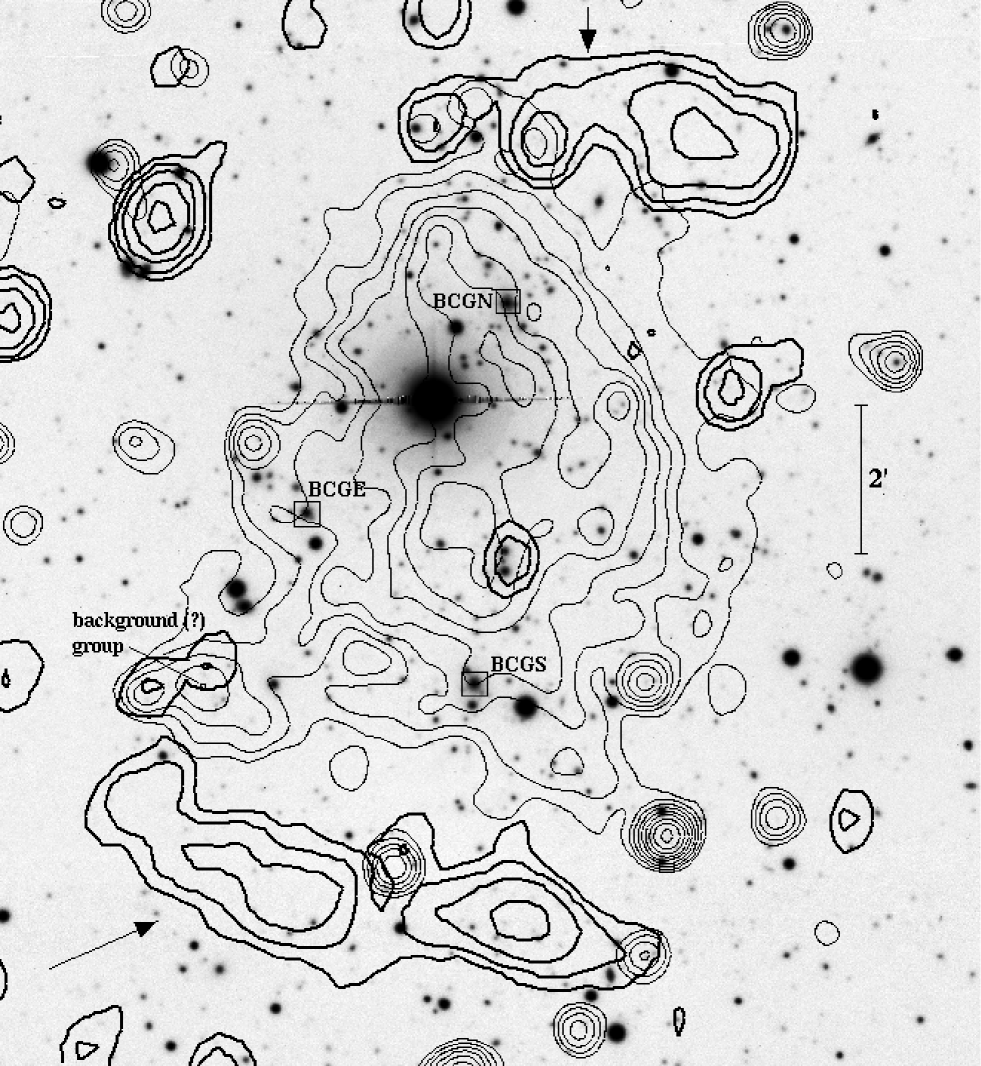
Figure 1: INT $R$–band image of the cluster A1240 (North at the top and East to the left) with, superimposed, the contour levels of the Chandra archival image ID 4961 (thin contours; photons in the energy range 0.5–2 keV) and the contour levels of a VLA radio image at 1.4 GHz (thick contours; Bonafede et al bon09 (2009)). Arrows show the positions of the two radio relics. Boxes highlight the brightest galaxies of A1240: BCGN, BCGS and BCGE (see text).

Unless otherwise stated, we give errors at the 68% confidence level (hereafter c.l.). Results with a c.l. below $90\%$ are considered very poorly/no significant. The values of these c.ls. are generally not explicitly listed throughout the paper.

Throughout this paper, we use $H_{0}=70$ km s^-1 Mpc^-1 in a flat cosmology with $\Omega_{0}=0.3$ and $\Omega_{\Lambda}=0.7$. In the adopted cosmology, 1$\mathrm{{}^{\prime}}\;$corresponds to $\sim 194$ $\mathrm{h_{70}^{-1}}$ kpc  at the cluster redshift.

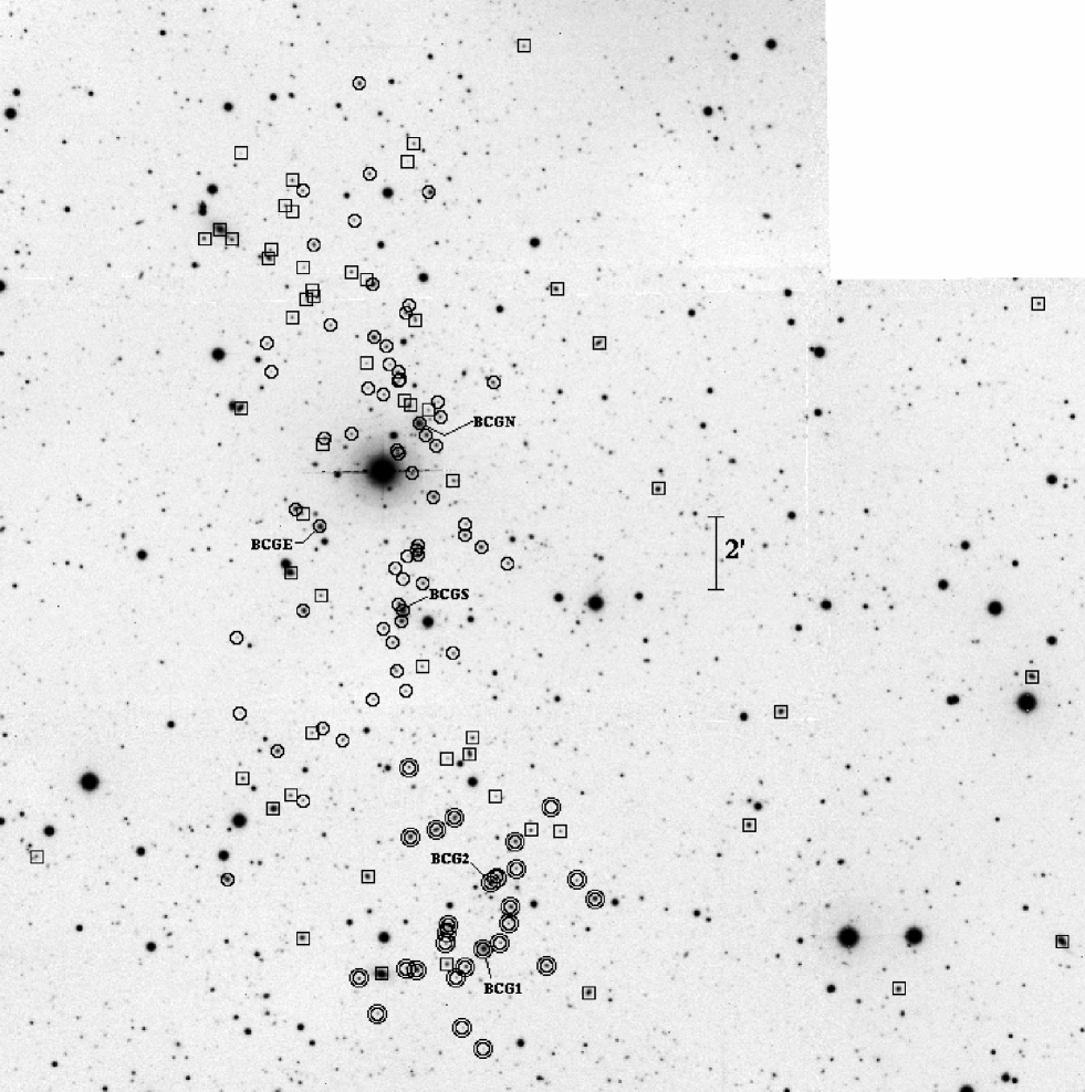
Figure 2: INT $R$–band image of the A1237+A1240 complex (North at the top and East to the left). Circles and annuli indicate cluster members of A1240 and A1237, respectively (see Table 1). Boxes indicate non–member galaxies.

2 New data and galaxy catalog

Multi–object spectroscopic observations of A1240 were carried out at the TNG telescope in December 2006 and December 2007. We used DOLORES/MOS with the LR–B Grism 1, yielding a dispersion of 187 Å/mm. In December 2006 we used the old Loral CCD, with a pixel size of 15 $\mu$m, while in December 2007 we used the new E2V CCD, with a pixel size of 13.5 $\mu$m. Both the CCDs are matrices of $2048\times 2048$ pixels. In total we observed four MOS masks (2 in 2006 and 2 in 2007) for a total of 142 slits. We acquired three exposures of 1800 s for each mask. Wavelength calibration was performed using Helium–Argon lamps. Reduction of spectroscopic data was carried out with the IRAF package.

Radial velocities were determined using the cross–correlation technique (Tonry & Davis ton79 (1979)) implemented in the RVSAO package (developed at the Smithsonian Astrophysical Observatory Telescope Data Center). Each spectrum was correlated against six templates for a variety of galaxy spectral types: E, S0, Sa, Sb, Sc, Ir (Kennicutt ken92 (1992)). The template producing the highest value of $\cal R$, i.e., the parameter given by RVSAO and related to the signal–to–noise ratio of the correlation peak, was chosen. Moreover, all spectra and their best correlation functions were examined visually to verify the redshift determination. In 4 cases (IDs 55, 61, 69, 129, 137; see Table 1) we took the EMSAO redshift as a reliable estimate of the redshift. Our spectroscopic survey in the field of A1240 consists of spectra for 118 galaxies with a median nominal error on $cz$ of 50 km s^-1. The nominal errors as given by the cross–correlation are known to be smaller than the true errors (e.g., Malumuth et al. mal92 (1992); Bardelli et al. bar94 (1994); Ellingson & Yee ell94 (1994); Quintana et al. qui00 (2000); Boschin et al. bos04 (2004)). Double redshift determinations for four galaxies allowed us to estimate real intrinsic errors. We compared the first and second determinations computing the mean and the rms of the variable $(z_{1}-z_{2})/\sqrt{err_{1}^{2}+err_{2}^{2}}$. We obtained $mean=0.3\pm 1.4$ and $rms=2.8$, to be compared with the expected values of 0 and 1. The resulting mean shows that the two sets of measurements are consistent with having the same velocity zero–point. According to the $\chi^{2}$–test the high value of the rms suggests that the errors are underestimated. Only when nominal errors are multiplied by a $\sim 2$ factor the rms is in acceptable agreement with the value of 1. Therefore, hereafter we assume that true errors are larger than nominal cross–correlation errors by a factor 2. For the four galaxies with two redshift estimates we used the weighted mean of the two measurements and the corresponding errors.

We also use 32 public redshift data as taken from NED within a box of 45x45$\mathrm{{}^{\prime}}\;$from the cluster center. They come from the SDSS (Data Release 7). Before to proceed with the merging between our and published catalogs we payed particular attention to their compatibility. Five galaxies are in common between SDSS and TNG data. For them we computed the mean and the rms of the variable $(z_{\rm our}-z_{\rm lit})/\sqrt{err_{\rm our}^{2}+err_{\rm lit}^{2}}$. We obtained $mean=-0.1\pm 0.6$ and $rms=1.5$, to be compared with the expected values of 0 and 1. The resulting mean shows that the two sets of measurements are consistent with having the same velocity zero–point, and the value of rms is compatible with a value of 1 according to the $\chi^{2}$–test. Thus we added the redshifts coming from the literature. For the five galaxies in common we used the weighted mean of the two redshift determinations and the corresponding errors. We obtained a final catalog of 145 galaxies with measured radial velocities.

As far as photometry is concerned, our observations were carried out with the Wide Field Camera (WFC), mounted at the prime focus of the 2.5m INT telescope. We observed the A1237+A1240 complex with $B_{\rm H}$ and $R_{\rm H}$ in photometric conditions. The $R$ image was obtained in December 19th 2004 with a seeing condition of 3.0$\mathrm{{}^{\prime}}\hskip-1.00006pt\mathrm{{}^{\prime}}$. We got the $B$ image in May 14th 2006 with a seeing of about 1.1$\mathrm{{}^{\prime}}\hskip-1.00006pt\mathrm{{}^{\prime}}$.

The WFC consists of a four–CCD mosaic covering a 33^′$\times$33$\mathrm{{}^{\prime}}\;$field of view, with only a 20% marginally vignetted area. We took nine exposures of 720 s in $B_{\rm H}$ and 300 s in $R_{\rm H}$ Harris filters (a total of 6480 s and 2700 s in each band) developing a dithering pattern of nine positions. This observing mode allowed us to build a “supersky” frame that was used to correct our images for fringing patterns (Gullixson gul92 (1992)). In addition, the dithering helped us to clean cosmic rays and avoid gaps between the CCDs in the final images. The complete reduction process (including flat fielding, bias subtraction and bad–column elimination) yielded a final coadded image where the variation of the sky was lower than 0.4% in the whole frame. Another effect associated with the wide field frames is the distortion of the field. In order to match the photometry of several filters, a good astrometric solution is needed to take into account these distortions. Using the $imcoords$ IRAF tasks and taking as a reference the USNO B1.0 catalog, we were able to find an accurate astrometric solution (rms $\sim$ 0.5$\mathrm{{}^{\prime}}\hskip-1.00006pt\mathrm{{}^{\prime}}$) across the full frame. The photometric calibration was performed using Landolt standard fields obtained during the observation.

We finally identified galaxies in our $B_{\rm H}$ and $R_{\rm H}$ images and measured their magnitudes with the SExtractor package (Bertin & Arnouts ber96 (1996)) and AUTOMAG procedure. In a few cases (e.g. close companion galaxies, galaxies close to defects of the CCD) the standard SExtractor photometric procedure failed. In these cases we computed magnitudes by hand. This method consists in assuming a galaxy profile of a typical elliptical galaxy and scaling it to the maximum observed value. The integration of this profile gives us an estimate of the magnitude. This method is similar to PSF photometry, but assumes a galaxy profile, more appropriate in this case.

We transformed all magnitudes into the Johnson–Cousins system (Johnson & Morgan joh53 (1953); Cousins cou76 (1976)). We used $B=B\rm_{H}+0.13$ and $R=R\rm_{H}$ as derived from the Harris filter characterization (http://www.ast.cam.ac.uk/$\sim$wfcsur/technical/photom/colours/) and assuming a $B-V\sim 1.0$ for E–type galaxies (Poggianti pog97 (1997)). As a final step, we estimated and corrected the galactic extinction $A_{B}\sim 0.10$, $A_{R}\sim 0.06$ from Burstein & Heiles’s (bur82 (1982)) reddening maps.

We estimated that our photometric sample is complete down to $R=20.5$ (22.0) and $B=22.0$ (23.0) for $S/N=5$ (3) within the observed field.

We assigned magnitudes to all galaxies of our spectroscopic catalog. We measured redshifts for galaxies down to magnitude $R\sim$ 20, but a high level of completeness is reached only for galaxies with magnitude $R<$ 19 ($\sim$45% completeness).

Table 1 lists the velocity catalog (see also Fig. 2): identification number of each galaxy, ID (Col. 1); right ascension and declination, $\alpha$ and $\delta$ (J2000, Col. 2); B and R magnitudes (Cols. 3 and 4); heliocentric radial velocities, ${\rm v}=cz_{\sun}$ (Col. 5) with errors, $\Delta{\rm v}$ (Col. 6); redshift source (Col. 7; T:TNG, S:SDSS); member assignment (Col. 8; 1:A1240, 2:A1237, 0:background/foreground).

Table 1: Velocity catalog of 145 spectroscopically measured galaxies in the field of the A1237+A1240 complex. In Col. 1, IDs 75, 56, 111, 29 and 27 (in boldface) highlight BCGS, BCGN, BCGE, BCG1 and BCG2, respectively (see text). Asterisks in Col. 8 highlight emission line galaxies.

$$\begin{array}[]{r c c r r r c r}\hline\cr\vskip 3.0pt plus 1.0pt minus 1.0pt\cr\hline\cr\vskip 3.0pt plus 1.0pt minus 1.0pt\cr\mathrm{ID}&\mathrm{\alpha},\mathrm{\delta}\,(\mathrm{J}2000)&B&R&\mathrm{v}&\mathrm{\Delta}\mathrm{v}&\mathrm{So.}&\mathrm{Cl.}\\ &&&&\mathrm{(\,km}&\mathrm{s^{-1}\,)}&&\\ \hline\cr\vskip 3.0pt plus 1.0pt minus 1.0pt\cr 1&11\ 22\ 00.12,+42\ 54\ 25.2&17.76&15.75&23230&53&\mathrm{S}&0\\ 2&11\ 22\ 03.36,+43\ 11\ 41.6&18.53&18.25&180587&338&\mathrm{S}&0\\ 3&11\ 22\ 04.44,+43\ 01\ 35.4&18.57&16.87&37090&40&\mathrm{S}&0\\ 4&11\ 22\ 24.24,+42\ 53\ 08.9&18.66&17.46&44576&27&\mathrm{S}&0\\ 5&11\ 22\ 41.52,+43\ 00\ 41.4&18.47&17.17&21546&49&\mathrm{S}&0\\ 6&11\ 22\ 46.20,+42\ 57\ 37.4&19.28&17.28&33915&46&\mathrm{S}&0\\ 7&11\ 22\ 59.88,+43\ 06\ 43.6&18.48&17.10&34993&32&\mathrm{S}&0\\ 8&11\ 23\ 08.52,+43\ 10\ 41.9&18.93&17.18&26827&42&\mathrm{S}&0\\ 9&11\ 23\ 09.24,+42\ 55\ 38.3&19.10&17.39&58448&31&\mathrm{S}&2\\ 10&11\ 23\ 10.32,+42\ 53\ 06.2&18.49&17.10&33987&41&\mathrm{S}&0\\ 11&11\ 23\ 11.96,+42\ 56\ 08.7&20.40&19.20&58737&78&\mathrm{T}&*2\\ 12&11\ 23\ 14.37,+42\ 57\ 28.6&21.00&19.34&90603&72&\mathrm{T}&*0\\ 13&11\ 23\ 15.00,+43\ 12\ 08.6&19.24&17.56&24005&30&\mathrm{S}&0\\ 14&11\ 23\ 15.76,+42\ 58\ 06.7&23.01&21.11&56786&150&\mathrm{T}&2\\ 15&11\ 23\ 16.45,+42\ 53\ 50.3&20.20&18.05&57516&56&\mathrm{T}&2\\ 16&11\ 23\ 18.74,+42\ 57\ 30.1&20.38&18.68&73676&88&\mathrm{T}&*0\\ 17&11\ 23\ 19.68,+43\ 18\ 44.6&21.96&18.84&133977&49&\mathrm{S}&0\\ 18&11\ 23\ 20.92,+42\ 56\ 28.3&21.40&19.08&57994&100&\mathrm{T}&2\\ 19&11\ 23\ 21.02,+42\ 57\ 12.5&19.58&17.91&57551&72&\mathrm{T}&2\\ 20&11\ 23\ 21.69,+42\ 55\ 25.9&20.22&17.83&57982&52&\mathrm{T}&2\\ 21&11\ 23\ 22.07,+42\ 54\ 58.6&21.64&19.22&59445&92&\mathrm{T}&2\\ 22&11\ 23\ 22.07,+43\ 04\ 44.2&20.81&18.64&59551&83&\mathrm{T}&1\\ 23&11\ 23\ 23.23,+42\ 54\ 27.7&21.22&19.03&58431&82&\mathrm{T}&2\\ 24&11\ 23\ 23.70,+42\ 56\ 13.9&20.29&17.88&58813&38&\mathrm{T}&2\\ 25&11\ 23\ 23.88,+42\ 58\ 25.7&23.49&19.78&90451&142&\mathrm{T}&*0\\ 26&11\ 23\ 24.26,+43\ 09\ 38.1&20.57&18.12&59406&140&\mathrm{T}&1\\ \textbf{27}&11\ 23\ 24.64,+42\ 56\ 06.0&19.46&16.92&57965&38&\mathrm{T+S}&2\\ 28&11\ 23\ 25.78,+42\ 51\ 34.7&22.14&20.45&58742&120&\mathrm{T}&2\\ \textbf{29}&11\ 23\ 25.80,+42\ 54\ 17.6&19.04&16.49&57482&52&\mathrm{S}&2\\ 30&11\ 23\ 26.04,+43\ 05\ 10.5&20.18&17.86&59031&50&\mathrm{T}&1\\ 31&11\ 23\ 27.35,+43\ 00\ 00.9&20.28&18.34&35290&70&\mathrm{T}&0\\ 32&11\ 23\ 27.80,+42\ 59\ 35.0&18.51&17.22&17883&26&\mathrm{T+S}&*0\\ 33&11\ 23\ 28.33,+43\ 05\ 48.1&21.23&19.27&57149&174&\mathrm{T}&1\\ 34&11\ 23\ 28.35,+42\ 53\ 49.1&20.77&18.52&57489&36&\mathrm{T}&2\\ 35&11\ 23\ 28.43,+43\ 05\ 29.9&20.49&18.22&57988&61&\mathrm{T}&1\\ \vskip 3.0pt plus 1.0pt minus 1.0pt\cr\hline\cr\vskip 3.0pt plus 1.0pt minus 1.0pt\cr\hline\cr\end{array}$$

Table 1: Continued.

$$\begin{array}[]{r c c r r r c r}\hline\cr\vskip 3.0pt plus 1.0pt minus 1.0pt\cr\hline\cr\vskip 3.0pt plus 1.0pt minus 1.0pt\cr\mathrm{ID}&\mathrm{\alpha},\mathrm{\delta}\,(\mathrm{J}2000)&B&R&\mathrm{v}&\mathrm{\Delta}\mathrm{v}&\mathrm{So.}&\mathrm{Cl.}\\ &&&&\mathrm{(\,km}&\mathrm{s^{-1}\,)}&&\\ \hline\cr\vskip 3.0pt plus 1.0pt minus 1.0pt\cr 36&11\ 23\ 28.81,+42\ 52\ 09.7&21.81&20.33&56626&86&\mathrm{T}&2\\ 37&11\ 23\ 29.80,+42\ 53\ 31.6&21.82&19.72&58741&54&\mathrm{T}&2\\ 38&11\ 23\ 29.97,+42\ 57\ 51.3&19.90&17.63&58621&142&\mathrm{T}&2\\ 39&11\ 23\ 30.13,+43\ 06\ 58.6&21.41&18.79&97901&128&\mathrm{T}&0\\ 40&11\ 23\ 30.17,+43\ 02\ 18.2&20.45&18.67&57717&112&\mathrm{T}&1\\ 41&11\ 23\ 30.84,+42\ 54\ 55.8&19.71&17.30&57368&43&\mathrm{S}&2\\ 42&11\ 23\ 31.07,+42\ 59\ 27.6&21.74&19.63&102577&106&\mathrm{T}&0\\ 43&11\ 23\ 31.17,+42\ 53\ 53.3&19.30&18.16&44948&88&\mathrm{T}&*0\\ 44&11\ 23\ 31.20,+42\ 54\ 45.8&19.84&17.54&59205&60&\mathrm{T}&2\\ 45&11\ 23\ 31.32,+42\ 54\ 26.3&21.30&19.31&59217&84&\mathrm{T}&2\\ 46&11\ 23\ 32.10,+43\ 08\ 42.0&20.75&18.41&57592&81&\mathrm{T}&1\\ 47&11\ 23\ 32.40,+43\ 09\ 06.8&22.03&19.59&58446&76&\mathrm{T}&1\\ 48&11\ 23\ 32.68,+43\ 07\ 56.0&20.83&18.79&58949&148&\mathrm{T}&1\\ 49&11\ 23\ 32.75,+42\ 57\ 31.8&19.75&17.60&57246&68&\mathrm{T}&2\\ 50&11\ 23\ 33.08,+43\ 06\ 32.2&20.18&17.86&59329&150&\mathrm{T}&1\\ 51&11\ 23\ 33.72,+43\ 14\ 47.4&19.67&17.25&59070&49&\mathrm{S}&1\\ 52&11\ 23\ 33.84,+43\ 08\ 53.3&20.96&18.62&84868&112&\mathrm{T}&*0\\ 53&11\ 23\ 34.15,+43\ 08\ 12.9&20.35&18.07&57839&128&\mathrm{T}&1\\ 54&11\ 23\ 34.67,+43\ 04\ 12.1&20.50&18.24&58620&64&\mathrm{T}&1\\ 55&11\ 23\ 34.82,+43\ 01\ 56.9&20.14&19.22&23909&87&\mathrm{T}&*0\\ \textbf{56}&11\ 23\ 35.26,+43\ 08\ 31.7&18.74&16.22&58353&96&\mathrm{T}&1\\ 57&11\ 23\ 35.46,+43\ 04\ 57.7&19.57&16.97&58717&46&\mathrm{T+S}&1\\ 58&11\ 23\ 35.48,+43\ 05\ 13.7&19.84&17.23&58230&100&\mathrm{T}&1\\ 59&11\ 23\ 35.52,+42\ 53\ 43.8&19.23&17.46&58805&43&\mathrm{S}&2\\ 60&11\ 23\ 35.60,+43\ 05\ 06.1&20.79&18.93&58415&180&\mathrm{T}&1\\ 61&11\ 23\ 35.77,+43\ 11\ 19.2&20.99&18.80&88635&156&\mathrm{T}&*0\\ 62&11\ 23\ 36.00,+43\ 16\ 06.3&21.02&18.99&53996&94&\mathrm{T}&0\\ 63&11\ 23\ 36.34,+43\ 07\ 11.1&20.99&18.77&58358&204&\mathrm{T}&1\\ 64&11\ 23\ 36.56,+42\ 57\ 20.5&19.67&17.58&56715&78&\mathrm{T}&2\\ 65&11\ 23\ 36.68,+43\ 09\ 01.9&20.38&18.00&60953&116&\mathrm{T}&0\\ 66&11\ 23\ 36.77,+42\ 59\ 13.5&21.03&18.88&57097&84&\mathrm{T}&2\\ 67&11\ 23\ 36.77,+43\ 11\ 44.5&20.99&19.00&59749&92&\mathrm{T}&1\\ 68&11\ 23\ 36.88,+43\ 04\ 56.3&22.13&19.75&59656&192&\mathrm{T}&1\\ 69&11\ 23\ 36.91,+43\ 15\ 37.3&22.17&20.82&153440&130&\mathrm{T}&*0\\ 70&11\ 23\ 37.16,+42\ 53\ 46.7&20.28&18.81&56870&74&\mathrm{T}&*2\\ \vskip 3.0pt plus 1.0pt minus 1.0pt\cr\hline\cr\vskip 3.0pt plus 1.0pt minus 1.0pt\cr\hline\cr\end{array}$$

Table 1: Continued.

$$\begin{array}[]{r c c r r r c r}\hline\cr\vskip 3.0pt plus 1.0pt minus 1.0pt\cr\hline\cr\vskip 3.0pt plus 1.0pt minus 1.0pt\cr\mathrm{ID}&\mathrm{\alpha},\mathrm{\delta}\,(\mathrm{J}2000)&B&R&\mathrm{v}&\mathrm{\Delta}\mathrm{v}&\mathrm{So.}&\mathrm{Cl.}\\ &&&&\mathrm{(\,km}&\mathrm{s^{-1}\,)}&&\\ \hline\cr\vskip 3.0pt plus 1.0pt minus 1.0pt\cr 71&11\ 23\ 37.17,+43\ 11\ 31.4&20.36&18.15&58635&142&\mathrm{T}&1\\ 72&11\ 23\ 37.28,+43\ 01\ 16.6&21.38&19.31&59878&70&\mathrm{T}&1\\ 73&11\ 23\ 37.34,+43\ 09\ 10.2&21.47&19.01&100284&258&\mathrm{T}&0\\ 74&11\ 23\ 37.53,+43\ 04\ 19.9&21.90&19.79&57709&118&\mathrm{T}&1\\ \textbf{75}&11\ 23\ 37.69,+43\ 03\ 28.2&18.82&16.12&58817&54&\mathrm{T}&1\\ 76&11\ 23\ 37.83,+43\ 03\ 10.8&19.76&17.11&56550&78&\mathrm{T}&1\\ 77&11\ 23\ 38.13,+43\ 09\ 43.9&20.84&19.42&60307&194&\mathrm{T}&*1\\ 78&11\ 23\ 38.22,+43\ 03\ 38.6&20.23&18.01&59542&92&\mathrm{T}&1\\ 79&11\ 23\ 38.32,+43\ 09\ 39.9&21.24&19.26&58342&140&\mathrm{T}&1\\ 80&11\ 23\ 38.35,+43\ 07\ 42.0&20.78&18.53&57397&53&\mathrm{T}&1\\ 81&11\ 23\ 38.37,+43\ 09\ 55.0&20.80&19.91&59828&148&\mathrm{T}&1\\ 82&11\ 23\ 38.46,+43\ 07\ 48.2&20.90&19.57&58605&200&\mathrm{T}&1\\ 83&11\ 23\ 38.63,+43\ 01\ 49.1&21.23&18.87&58509&80&\mathrm{T}&1\\ 84&11\ 23\ 38.85,+43\ 04\ 36.8&20.57&19.33&55562&134&\mathrm{T}&*1\\ 85&11\ 23\ 39.15,+43\ 02\ 35.5&20.77&18.73&57478&78&\mathrm{T}&1\\ 86&11\ 23\ 39.54,+43\ 10\ 07.4&22.07&19.63&58711&146&\mathrm{T}&1\\ 87&11\ 23\ 40.08,+43\ 10\ 36.4&20.74&18.37&57351&160&\mathrm{T}&1\\ 88&11\ 23\ 40.47,+43\ 09\ 18.7&21.41&18.97&59078&94&\mathrm{T}&1\\ 89&11\ 23\ 40.50,+43\ 02\ 59.3&20.92&18.79&56851&82&\mathrm{T}&1\\ 90&11\ 23\ 40.87,+42\ 53\ 37.4&17.00&15.19&23141&37&\mathrm{T+S}&0\\ 91&11\ 23\ 41.42,+42\ 52\ 33.5&20.59&19.47&58938&118&\mathrm{T}&*2\\ 92&11\ 23\ 41.92,+43\ 10\ 51.7&19.76&17.41&57628&138&\mathrm{T}&1\\ 93&11\ 23\ 42.04,+43\ 01\ 03.9&21.19&19.61&56216&120&\mathrm{T}&1\\ 94&11\ 23\ 42.05,+43\ 12\ 17.8&19.45&17.16&57828&42&\mathrm{T+S}&1\\ 95&11\ 23\ 42.60,+43\ 15\ 17.3&20.91&18.65&59502&120&\mathrm{T}&1\\ 96&11\ 23\ 42.85,+43\ 09\ 29.3&22.03&19.57&57407&144&\mathrm{T}&1\\ 97&11\ 23\ 42.89,+43\ 12\ 24.4&21.43&18.91&90672&92&\mathrm{T}&0\\ 98&11\ 23\ 42.94,+42\ 56\ 16.2&18.87&17.55&23440&94&\mathrm{T}&*0\\ 99&11\ 23\ 43.03,+43\ 10\ 09.4&21.59&19.79&90196&186&\mathrm{T}&0\\ 100&11\ 23\ 44.16,+43\ 17\ 44.5&18.97&17.96&59099&29&\mathrm{S}&1\\ 101&11\ 23\ 44.19,+42\ 53\ 30.4&21.03&18.45&57649&46&\mathrm{T}&2\\ 102&11\ 23\ 44.90,+43\ 14\ 02.4&21.25&19.06&59238&186&\mathrm{T}&1\\ 103&11\ 23\ 45.26,+43\ 08\ 14.8&21.35&19.93&56860&110&\mathrm{T}&1\\ 104&11\ 23\ 45.29,+43\ 12\ 38.4&21.18&18.88&98761&94&\mathrm{T}&0\\ 105&11\ 23\ 46.58,+42\ 59\ 57.6&20.57&18.78&56478&76&\mathrm{T}&1\\ \vskip 3.0pt plus 1.0pt minus 1.0pt\cr\hline\cr\vskip 3.0pt plus 1.0pt minus 1.0pt\cr\hline\cr\end{array}$$

Table 1: Continued.

$$\begin{array}[]{r c c r r r c r}\hline\cr\vskip 3.0pt plus 1.0pt minus 1.0pt\cr\hline\cr\vskip 3.0pt plus 1.0pt minus 1.0pt\cr\mathrm{ID}&\mathrm{\alpha},\mathrm{\delta}\,(\mathrm{J}2000)&B&R&\mathrm{v}&\mathrm{\Delta}\mathrm{v}&\mathrm{So.}&\mathrm{Cl.}\\ &&&&\mathrm{(\,km}&\mathrm{s^{-1}\,)}&&\\ \hline\cr\vskip 3.0pt plus 1.0pt minus 1.0pt\cr 106&11\ 23\ 48.35,+43\ 11\ 11.6&20.54&18.95&58801&84&\mathrm{T}&*1\\ 107&11\ 23\ 49.20,+43\ 08\ 07.9&20.39&18.30&57904&118&\mathrm{T}&1\\ 108&11\ 23\ 49.42,+43\ 00\ 17.4&21.08&18.78&58494&116&\mathrm{T}&1\\ 109&11\ 23\ 49.54,+43\ 07\ 59.1&22.51&20.07&84937&196&\mathrm{T}&0\\ 110&11\ 23\ 49.83,+43\ 03\ 52.8&21.37&18.79&91883&118&\mathrm{T}&0\\ \textbf{111}&11\ 23\ 49.92,+43\ 05\ 44.7&19.21&16.72&56134&66&\mathrm{T}&1\\ 112&11\ 23\ 50.86,+43\ 13\ 22.2&21.25&19.06&59144&104&\mathrm{T}&1\\ 113&11\ 23\ 51.09,+43\ 12\ 01.0&21.51&19.94&61506&118&\mathrm{T}&0\\ 114&11\ 23\ 51.14,+43\ 00\ 09.2&20.62&19.24&48223&126&\mathrm{T}&*0\\ 115&11\ 23\ 51.15,+43\ 12\ 06.5&20.98&19.59&78030&138&\mathrm{T}&*0\\ 116&11\ 23\ 51.87,+43\ 11\ 54.8&20.96&18.85&152164&138&\mathrm{T}&0\\ 117&11\ 23\ 52.35,+43\ 12\ 45.5&21.11&19.50&55225&94&\mathrm{T}&0\\ 118&11\ 23\ 52.44,+42\ 54\ 36.4&18.55&17.45&23511&28&\mathrm{S}&0\\ 119&11\ 23\ 52.44,+43\ 03\ 28.1&19.62&17.15&58336&48&\mathrm{S}&1\\ 120&11\ 23\ 52.47,+42\ 58\ 19.6&21.25&19.12&58639&86&\mathrm{T}&1\\ 121&11\ 23\ 52.51,+43\ 14\ 50.0&20.93&18.83&59284&104&\mathrm{T}&1\\ 122&11\ 23\ 52.59,+43\ 06\ 05.3&22.05&19.03&84545&166&\mathrm{T}&0\\ 123&11\ 23\ 53.52,+43\ 06\ 13.3&19.76&17.30&59022&47&\mathrm{S}&1\\ 124&11\ 23\ 54.07,+43\ 15\ 07.2&20.21&18.63&21528&86&\mathrm{T}&0\\ 125&11\ 23\ 54.10,+43\ 11\ 24.4&20.63&18.97&77906&94&\mathrm{T}&*0\\ 126&11\ 23\ 54.21,+43\ 14\ 17.2&21.87&19.94&106774&98&\mathrm{T}&0\\ 127&11\ 23\ 54.31,+42\ 58\ 28.1&20.48&18.59&87022&90&\mathrm{T}&0\\ 128&11\ 23\ 54.60,+43\ 04\ 30.0&17.76&16.07&21275&45&\mathrm{S}&0\\ 129&11\ 23\ 55.13,+43\ 14\ 26.0&19.61&18.90&24046&30&\mathrm{T}&*0\\ 130&11\ 23\ 56.24,+42\ 59\ 40.4&19.98&17.58&58805&68&\mathrm{T}&1\\ 131&11\ 23\ 56.76,+42\ 58\ 06.2&18.00&16.57&23303&31&\mathrm{S}&0\\ 132&11\ 23\ 57.23,+43\ 09\ 56.6&21.71&20.56&58966&130&\mathrm{T}&*1\\ 133&11\ 23\ 57.48,+43\ 13\ 13.8&21.14&18.78&331328&450&\mathrm{S}&0\\ 134&11\ 23\ 57.57,+43\ 13\ 01.2&19.36&17.22&54792&80&\mathrm{T}&0\\ 135&11\ 23\ 57.81,+43\ 10\ 41.5&21.44&19.24&58346&156&\mathrm{T}&1\\ 136&11\ 24\ 01.38,+42\ 58\ 55.5&20.18&18.45&48099&74&\mathrm{T}&0\\ 137&11\ 24\ 01.72,+43\ 15\ 50.5&21.28&20.33&78070&71&\mathrm{T}&*0\\ 138&11\ 24\ 01.75,+43\ 00\ 42.0&21.17&19.56&57426&144&\mathrm{T}&*1\\ 139&11\ 24\ 01.80,+43\ 08\ 57.5&17.77&16.31&21326&56&\mathrm{S}&0\\ 140&11\ 24\ 02.20,+43\ 02\ 44.4&22.03&19.78&56604&212&\mathrm{T}&1\\ 141&11\ 24\ 03.24,+43\ 13\ 30.7&19.66&18.04&96076&37&\mathrm{S}&0\\ 142&11\ 24\ 03.60,+42\ 56\ 11.4&19.51&17.03&58204&46&\mathrm{S}&1\\ 143&11\ 24\ 04.83,+43\ 13\ 48.0&17.54&15.48&21158&112&\mathrm{T}&0\\ 144&11\ 24\ 07.19,+43\ 13\ 32.7&20.41&18.03&55467&102&\mathrm{T}&0\\ 145&11\ 24\ 31.68,+42\ 56\ 49.6&21.16&18.28&92075&75&\mathrm{S}&0\\ \vskip 3.0pt plus 1.0pt minus 1.0pt\cr\hline\cr\vskip 3.0pt plus 1.0pt minus 1.0pt\cr\hline\cr\end{array}$$

3 Analysis and Results

3.1 Member selection

To select cluster members out of 145 galaxies having redshifts, we follow a two steps procedure. First, we perform the 1D adaptive–kernel method (hereafter DEDICA, Pisani pis93 (1993) and pis96 (1996); see also Fadda et al. fad96 (1996); Girardi et al. gir96 (1996)). We search for significant peaks in the velocity distribution at $>$99% c.l.. This procedure detects A1237+A1240 as a peak at $z\sim 0.196$ populated by 95 galaxies considered as candidate cluster members (see Fig. 3). Out of 50 non members, 24 and 26 are foreground and background galaxies, respectively.

Figure 3: Redshift galaxy distribution. The solid line histogram refers to the 95 galaxies assigned to the A1237+A1240 complex according to the DEDICA reconstruction method.

All the galaxies assigned to the cluster peak are analyzed in the second step which uses the combination of position and velocity information: the “shifting gapper” method by Fadda et al. (fad96 (1996)). This procedure rejects galaxies that are too far in velocity from the main body of galaxies within a fixed bin that shifts along the distance from the cluster center. The procedure is iterated until the number of cluster members converges to a stable value. Following Fadda et al. (fad96 (1996)) we use a gap of $1000$ km s${}^{-1}\;$– in the cluster rest–frame – and a bin of 0.6 $h_{70}^{-1}$ Mpc, or large enough to include 15 galaxies.

The choice of the center of A1240 is not obvious. No evident dominant galaxy is present, rather there are some luminous galaxies. In particular, the two brightest ones, ID. 75 and ID. 56, lie in the southern and northern region of A1240, respectively, and show comparable luminosity (hereafter BCGS and BCGN). The third one is located in the eastern region, but is $\gtrsim 0.5$ $R$–magnitudes fainter than BCGS and BCGN (ID. 111, hereafter BCGE). As for the cluster center, hereafter we assume the position of the centroid of the X–ray emission as recovered by David et al. (dav99 (1999)) [R.A.=$11^{\mathrm{h}}23^{\mathrm{m}}37\,\hbox to0.0pt{\hbox{$\mathrm{{}^{s}}$}\hss}{\hbox{$.$}}\,6$, Dec.=$+43\mathrm{{}^{\circ}}05\mathrm{{}^{\prime}}51\mathrm{{}^{\prime}}\hskip-1.00006pt\mathrm{{}^{\prime}}\;$ (J2000.0)] which lies between the two dominant galaxies. After the “shifting gapper” procedure we obtain a sample of 89 fiducial cluster members (see Fig. 4).

Figure 4: Rest–frame velocity vs. projected clustercentric distance for the 95 galaxies in the main peak (Fig. 3) showing galaxies detected as interlopers by our “shifting gapper” procedure (crosses). Circles indicate the 89 cluster members.

We also check the result of alternative member selection procedures. We apply the “shifting gapper” procedure adopting as cluster center the brightest cluster galaxy (BCGS). We find a cluster sample of 89 galaxies, 88 of which are in common with our above sample. In order to analyze the effect of a fully alternative selection procedure we also apply the classical 3–$\sigma$ clipping procedure by Yahil & Vidal (1977) on the whole sample of 145 galaxies after a very rough cut in the velocity space, i.e. rejecting galaxies with velocities differing by more than 8000 km s${}^{-1}\;$from the mean velocity. This classical procedure leads to a sample of 90 galaxies, 89 of which forms our adopted sample. In conclusion, the sample of member galaxies we adopt in this work is quite robust against the member selection procedure.

The galaxy distribution analyzed through the 2D DEDICA method clearly shows the presence of a southern external clump (see Fig. 5, see also Sect. 3.7). Gal et al. (gal03 (2003)) recovered a cluster in the same position from the digitized Second Palomar Observatory Sky Survey. We identify this galaxy clump with A1237 which is likely to have a cluster redshift similar to that of A1240 (cf. the magnitudes of their 10th–ranked cluster galaxies, Abell et al. abe89 (1989)). Notice that the center reported by Abell et al. is quite imprecise and lies on the southern border of the galaxy concentration we detect.

Figure 5: Spatial distribution on the sky and relative isodensity contour map of cluster members (A1237+A1240), obtained with the DEDICA method. The positions of the brightest galaxies are indicated (BCGN, BCGS, BCGE for A1240 and BCG1 and BCG2 for A1237). The plot is centered on the cluster center defined in this paper as the X–ray center. The two relics are indicated in a schematic way.

We use the 2D DEDICA results, i.e. the peaks detected in the 2D galaxy distribution, to assign galaxies to different subclumps. The 2D DEDICA algorithm detects nine peaks, four of which are more significant than the $99\%$ c.l.. The southern three peaks, only one of which is very significant, are assigned to A1237 (for a total of 27 members). The six northern peaks, three of which are very significant, are assigned to A1240 (for a total of 62 members). This assignment is shown in Fig. 6 – left panel.

As for A1240, the 2D DEDICA algorithm shows a clear bimodal structure (see Fig. 5) along the North-South direction. This bimodality is also shown in our analysis of photometric “likely” members in Sect. 3.7 and corresponds to the elongated hot gas distribution shown by the previous analyses of ROSAT data (David et al. dav99 (1999); Bonafede et al. bon09 (2009)) and our analysis of Chandra data (see Sect. 4). Therefore we decide to consider: a southern structure – hereafter A1240S – associated to the southern peak of A1240 (the most significant in the whole DEDICA analysis); a northern structure – hereafter a1240N – associated to the four northern peaks (two of which are very significant). In this way we assign 32 (27) members to A1240N (A1240S). A1240S and A1240N host the brightest and the second brightest galaxies, BCGS and BCGN, respectively. We consider separately three galaxies belonging to a minor, eastern peak (hereafter A1240E) since their assignation to A1240N or A1240S is not obvious. A1240E hosts the BCGE. The assignment of galaxies within A1240 is summarized as follow: we assign to A1240S the galaxies belonging to the southern peak (detected with a $>99.99\%$ c.l.); to A1240N the galaxies belonging to the four, northern peaks (two of which are detected with a $>99.8\%$ c.l.); to a1240E the galaxies belonging to the eastern peak.

Figure 6: Spatial distribution on the sky of 89 cluster members. Left panel: open symbols indicate cluster members. In particular, squares, circles, rotated squares and triangles indicate A1240N, A1240S, A1240E and A1237. The crosses indicate emission line galaxies. Right panel: the larger the symbol, the smaller is the radial velocity. The six close northern circles indicate the high velocity galaxies we consider responsible of the apparent large global mean velocity of A1240N galaxies (see Sect. 3.4 and Fig. 10 in the following, too).

3.2 The A1237+A1240 complex in the velocity space

According to the 1D Kolmogorov–Smirnov test (hereafter 1DKS–test; see, e.g., Press et al pre92 (1992)), there is no significant difference between the velocity distributions of A1237 and A1240 (see also Fig. 6 – right panel). This result suggests us to investigate the global velocity distribution of the complex.

We analyze the velocity distribution of cluster galaxies (see Fig. 7) using a few tests where the null hypothesis is that the velocity distribution is a single Gaussian. We estimate three shape estimators: the kurtosis, the skewness, and the scaled tail index (see, e.g., Beers et al. bee91 (1991)). According to the value of the skewness (-0.379) the velocity distribution is marginally asymmetric differing from a Gaussian at the $90-95\%$ c.l. (see Table 2 of Bird & Beers bir93 (1993)). We also analyze the presence of “weighted gaps” in the velocity distribution. A weighted gap in the space of the ordered velocities is defined as the difference between two contiguous velocities, weighted by the location of these velocities with respect to the middle of the data (Wainer and Schacht wai78 (1978); Beers et al. bee91 (1991)). We detect a strongly significant gap (at the $>99.9\%$ c.l.) and five minor gaps (at the $\gtrsim 98\%$ c.l.), see Fig. 7 – lower panel. The most important gap, very significant since it is located in the central region of the velocity distribution, separates the cluster into two subgroups of 37 and 52 galaxies. When comparing the 2D galaxy distributions of these subgroups we find no difference according to the 2D Kolmogorov–Smirnov test (Fasano & Franceschini fas87 (1987)).

Figure 7: Upper panel: velocity histogram for the whole cluster sample (thin line), A1240 (solid line) and A1237 (dashed line). The velocities of the three brightest galaxies of A1240 are indicated (BCGN, BCGS and BCGE), as well as the two brightest galaxies of A1237 (BCG1 and BCG2). Lower panel: stripe density plot where the arrows indicate the positions of the significant gaps. The main and minor weighted gaps are indicated by big and small arrows, respectively.

We also perform the 2D and 3D Kaye’s mixture model (KMM) test (as implemented by Ashman et al. ash94 (1994)) and compare the results to check the effect of the addition of the velocity information. The KMM algorithm fits a user–specified number of Gaussian distributions to a dataset and assesses the improvement of that fit over a single Gaussian and give an assignment of objects into groups. We use the A1237+A1240 galaxy assignment found by the 2D DEDICA analysis to determine the first guess when fitting two groups. The 2D KMM algorithm fits a two–group partition, at the $>99.9\%$ c.l. according to the likelihood ratio test, leading to two groups of 66 and 23 galaxies. The addition of the velocity information in the KMM algorithm leads to the same group partition.

Finally, we combine galaxy velocity and position information to compute the $\Delta$–statistics devised by Dressler & Shectman (dre88 (1988)). This test is sensitive to spatially compact subsystems that have either an average velocity that differs from the cluster mean, or a velocity dispersion that differs from the global one, or both. We find no significant substructure.

We conclude that, although the velocity distribution shows evidence of a complex structure, A1237 and A1240 are so similar in the velocity space that the velocity information is not useful to improve the galaxy assignment recovered from the 2D analysis (see Sect. 3.1).

3.3 Global Kinematical properties

As for the whole cluster complex, by applying the biweight estimator to the 89 members (Beers et al. bee90 (1990)), we compute a mean redshift of $\left<z\right>=0.1937\pm$ 0.0003, i.e. $\left<\rm{v}\right>=(58273\pm 89)$ km s^-1. We estimate the LOS velocity dispersion, $\sigma_{\rm V}$, by using the biweight estimator and applying the cosmological correction and the standard correction for velocity errors (Danese et al. dan80 (1980)). We obtain $\sigma_{\rm V}=842_{-55}^{+63}$ km s^-1, where errors are estimated through a bootstrap technique.

The results obtained for the 62 members of A1240 are: $\left<z\right>=0.1948\pm$ 0.0004, i.e. $\left<\rm{v}\right>=(58408\pm 111)$ km s${}^{-1}\;$, and $\sigma_{\rm V}=870_{-79}^{+91}$ km s^-1. To evaluate the robustness of $\sigma_{\rm V}$ of A1240 we analyze the velocity dispersion profile (Fig. 8). The integral profile is roughly flat in the external cluster regions suggesting that the value of $\sigma_{\rm V}$ for A1240 is quite robust. Figure 8 also shows that the $\left<\rm{v}\right>$ and $\sigma_{\rm V}$ profiles are not disturbed by the presence of A1237.

Figure 8: Upper panel: rest–frame velocity (in units of $10^{3}$ km s^-1) vs. projected clustercentric distance for the 89 cluster galaxies. Circles and squares indicate members of A1240 and A1237. Central and lower panels: integral profiles of mean LOS velocity (in units of $10^{3}$ km s^-1) and LOS velocity dispersion (in units of km s^-1) for the 62 members of A1240 (dots with the $68\%$ c.l. errorbar) and for all the 89 cluster members (A1237+A1240, solid line). The mean and dispersion at a given (projected) radius from the cluster–center is estimated by considering all galaxies within that radius – the first value computed on the five galaxies closest to the center. In the lower panel, the horizontal lines represent the X–ray temperature with the respective $68\%$ errors transformed in $\sigma_{\rm V}$ assuming the density–energy equipartition between gas and galaxies, i.e. $\beta_{\rm spec}=1$ where $\beta_{\rm spec}=\sigma_{\rm V}^{2}/(kT/\mu m_{\rm p})$ with $\mu=0.58$ the mean molecular weight and $m_{\rm p}$ the proton mass. In all the panels the center is the X–ray center of A1240.

Table 2 lists the number of the member galaxies $N_{\rm g}$ and the main kinematical properties of A1237 and A1240.

Table 2: Global properties of galaxy systems.

$$\begin{array}[]{l c c c c c c}\hline\cr\vskip 3.0pt plus 1.0pt minus 1.0pt\cr\hline\cr\vskip 3.0pt plus 1.0pt minus 1.0pt\cr\mathrm{System}&N_{\rm g}&\alpha,\,\delta&\mathrm{<v>}&\sigma_{\rm V}&R_{\rm vir}&M(<R_{\rm vir})\\ &&({\rm J}2000)&\mathrm{km\ s^{-1}}&\mathrm{km\ s^{-1}}&h_{70}^{-1}{\rm Mpc}&h_{70}^{-1}10^{14}\mathrm{M}_{\odot}\\ \hline\cr\vskip 3.0pt plus 1.0pt minus 1.0pt\cr\mathrm{A1237}&27&112329.5+425419&58021\pm 145&738_{-54}^{+82}&1.6&6\pm 2\\ \mathrm{A1240}&62&112337.6+430551&58408\pm 111&870_{-79}^{+91}&1.9-2.4^{\mathrm{b}}&9-19^{\mathrm{b}}\\ \mathrm{A1240N^{\mathrm{a}}}&32&112335.2+430832&\sim 58353&709_{-83}^{+88}&1.6&5\pm 2\\ \mathrm{A1240S^{\mathrm{a}}}&27&112337.7+430328&\sim 58817&991_{-99}^{+149}&2.2&14\pm 5\\ \vskip 3.0pt plus 1.0pt minus 1.0pt\cr\hline\cr\vskip 3.0pt plus 1.0pt minus 1.0pt\cr\hline\cr\end{array}$$

• As center and mean velocity of this clump we list the position and velocity of the respective brightest galaxy.

• The lower limit comes from the observed $\sigma_{\rm V}$. The upper limit is obtained when considering the bimodal structure of the cluster (see text).

Figure 9 compares the $\left<\rm{v}\right>$ and $\sigma_{\rm V}$ profiles of A1240 and A1237, where for A1240 we show separately the results for A1240N and A1240S. The value $\left<\rm{v}\right>$ of A1237 is similar to that of A1240S, suggesting a continuity in the velocity field. However the value of $\sigma_{\rm V}$ of A1237 is clearly lower than that of A1240S, suggesting that A1237 is really a less massive system.

Figure 9: Upper panel: rest–frame velocity (in units of $10^{3}$ km s^-1) vs. projected clustercentric distance for the members of A1240N (squares), A1240S (circles) and A1237 (crosses). In this and other panels the lower axis give the clustercentric distance of A1240N (A1240S) galaxies versus the negative (positive) axis from the A1240 center, while the upper axis give the clustercentric distance of A1237 galaxies from the A1237 center. The center of A1240 is defined as the X–ray center. The center of A1237 is defined as the position of the main peak in the 2D analysis. Central and lower panels: $68\%$ error bands of integral profiles of LOS mean velocity (in units of $10^{3}$ km s^-1) and LOS velocity dispersion (in units of km s^-1) for A1240N and A1240S (solid lines) and A1237 (dashed lines). The circles in the central panel indicate the positions and velocities of the two brightest galaxies of A1240 (BCGN and BCGS) and the two brightest galaxies of A1237 (BCG1 and BCG2).

3.4 Internal structure of A1240

According to the 1DKS–test there is no difference between the velocity distributions of A1240N and A1240S. The velocity distribution of A1240 shows signatures of non–Gaussianity similar to those of the whole cluster complex (e.g. a slight asymmetry and an important gap, see Fig. 7). Like for the A1237 vs. A1240 case, we find that A1240N and A1240S are so similar in the velocity space that the velocity information is not useful to improve the galaxy assignment. However, at the contrary of the A1237 vs. A1240 case, A1240N and A1240S are spatially closer and likely strongly interacting (see Sect. 5). This suggests that the galaxy assignment might be questionable and that we must devote more cure in determining the individual kinematical properties of the two subclumps.

The value of global $\left<\rm{v}\right>$ of A1240N is nominally larger than that of A1240S, i.e. $\left<\rm{v}\right>=(58624\pm 128)$ km s${}^{-1}\;$and $\left<\rm{v}\right>=(58091\pm 195)$ km s${}^{-1}\;$respectively, only at a $\sim$ 2$\sigma$ c.l. Moreover, looking at Fig. 9, the two cores of A1240N and A1240S seem to have similar $\left<\rm{v}\right>$: this is better shown in Fig.10, where we directly compare the profiles of A1240N and A1240S. The large global $\left<\rm{v}\right>$ of A1240N is likely due to few high velocity galaxies in the extreme northern cluster regions (see the six galaxies shown as close circles in Fig. 6 – right panel; see also Fig. 10). Indeed, the recent merger of two subclumps may result in a plume, or arm, of outflying galaxies detected for their different velocity with respect to the cluster (see e.g. the case of Abell 3266; Quintana et al. qui96 (1999) and Flores et al. flo00 (2000)). Due to these difficulties in detecting a quantitative difference between A1240N and A1240S, we prefer to use the position and velocity of BCGN and BCGS as tracers of the two interveining clumps. In fact, dominant galaxies trace the cluster substructures (Beers & Geller bee83 (1983)) and are good tracers of interacting subclumps during a cluster merger, too (e.g., Boschin et al. bos06 (2006); Barrena et al. 2007a ; Boschin et al. bos09 (2009)).

The nominal value of global $\sigma_{\rm V}$ of A1240N is smaller than that of A1240S, $\sigma_{\rm V}=709_{-83}^{+88}$ km s${}^{-1}\;$and $\sigma_{\rm V}=991_{-99}^{+149}$ km s${}^{-1}\;$respectively. Using the brightest galaxies as centers the comparison of the respective $\sigma_{\rm V}$ profiles confirms this trend (see Fig.10 – right lower panel). Thus, although the nominal values of individual $\sigma_{\rm V}$ might be not fully reliable, we decide to adopt them for describing A1240N and A1240S.

Table 2 summarizes the properties of A1240N and A1240S.

Figure 10: Upper panels: Error bands of integral profiles of LOS mean velocity for A1240N (dashed line) and A1240S (solid line). The distance is computed using as the center the position of the most important peak (on the left) and the position of the brightest cluster member (on the right). The horizontal lines indicate the velocities of BCGN and BCGS (dashed and solid lines, respectively). The close circles point out at which radius the six northern high velocity galaxies in A1240N are included to show their effect on the estimate of the mean velocity (see the text and Fig. 6, too). Lower panels: The same for integral profiles of the LOS velocity dispersion.

3.5 Internal structure of A1237

As for A1237, it appears dominated by two bright galaxies, BCG1 and BCG2 (IDs. 29 and 27, see Table 1) and the 2D DEDICA algorithm shows the presence of one significant peak (at the $>99\%$ c.l.) and two minor peaks significant at the $97\%$ and $89\%$ c.l. (see the somewhat elongated structure of A1237 in Fig. 5). Both the analysis of SDSS and our photometric data show that A1237 has only one well defined peak in the 2D galaxy distribution (see Sect. 3.7). This last result is based on a much larger sample, thus we conclude that we have no evidence for a complex structure in A1237. The velocity distribution shows evidence for a platykurtic behavior, but at a poorly significant level (at the $\sim 95\%$ c.l.).

3.6 Mass estimates

Under the usual assumptions (cluster sphericity, dynamical equilibrium and galaxy distribution tracing the mass distribution), we can compute global virial quantities. Following the prescriptions of Girardi & Mezzetti (gir01 (2001)), the virial radius is $R_{\rm vir}=0.17\times\sigma_{\rm V}/H(z)$ $h_{70}^{-1}$ Mpc (see their Eq. 1 after introducing the scaling with $H(z)$; see also Eq.  8 of Carlberg et al. car97 (1997) for $R_{200}$) and the virial mass (Limber & Mathews lim60 (1960); see also, e.g., Girardi et al. gir98 (1998)) is:

$$M=3\pi/2\cdot\sigma_{\rm V}^{2}R_{\rm PV}/G-{\rm SPT}.$$ (1)

The quantity SPT, the surface pressure term correction (The & White the86 (1986)), is assumed to be equal to the $20\%$ of the mass since this is the typical value recovered for the mass computed within the virial radius in the literature when the data of many clusters are combined together to enlarge the statistics (Carlberg et al. car97 (1997); Girardi et al. gir98 (1998)). The quantity $R_{\rm PV}$ is a projected radius (equal to two times the projected harmonic radius). The value of $R_{\rm PV}$ depends on the size of the sampled region and possibly on the quality of the spatial sampling (e.g., whether the cluster is uniformly sampled or not). It is also possible to use an alternative estimate of $R_{\rm PV}$ based on a priori knowledge of the galaxy distribution (see the Appendix in Girardi et al. gir95 (1995)). Following Girardi et al. (gir98 (1998); see also Girardi & Mezzetti gir01 (2001)) we can assume a King–like distribution with parameters typical of nearby/medium–redshift clusters: a core radius $R_{\rm c}=1/20\times R_{\rm vir}$ and a slope–parameter $\beta_{\rm fit,gal}=0.8$, i.e., the volume galaxy density at large radii scales as $r^{-3\beta_{\rm fit,gal}}=r^{-2.4}$. With these assumptions we can use the eq. A6 of Girardi et al. (gir95 (1995)) to estimate $R_{\rm PV}$, see also eq. 13 of Girardi et al. gir98 (1998) for a useful approximation (i.e., $R_{\rm PV}=1.189R_{\rm vir}[1+0.053(R_{\rm vir}/R_{\rm c})]/[1+0.117(R_{\rm vir}/R_{\rm c})]$. Having assumed the galaxy distribution, the value of $R_{\rm PV}$ depends only on $R_{\rm vir}$. In this way our estimates of global virial quantities only depend on our estimate of $\sigma_{\rm V}$.

Through this procedure we obtain a mass estimate $M_{\rm A1237}(<R_{\rm vir}=1.63\;h_{70}^{-1}\mathrm{Mpc})=(6\pm 2)$ $\times 10^{14}\;h_{70}^{-1}\;M_{\odot}\;$and $M_{\rm A1240}(<R_{\rm vir}=1.92\;h_{70}^{-1}\mathrm{Mpc})=(9\pm 3)$ $\times 10^{14}\;h_{70}^{-1}\;M_{\odot}$.

When a cluster shows a strongly substructured appearance (e.g., a bimodal structure), the use of the global $\sigma_{\rm V}$ to compute the mass might be misleading (Girardi et al. gir97 (1997) and refs. therein). The true mass could be overestimated or underestimated depending on the angle of view of the cluster structure. When the two subclumps are aligned along the LOS, they cannot be clearly distinguished in their projection onto the sky, but they can appear as two peaks (less or more overlapped, depending on their relative velocity) in the redshift distribution: in this case the mass estimated by the observed global $\sigma_{\rm V}$ is likely to be an overestimate of the true cluster mass (e.g., cf. Tabs. 7 and  8 of Girardi et al. gir98 (1998)). When the two subclumps are aligned along an axis parallel to the plane of sky, they appear as two structures in their projection onto the sky but they cannot be distinguished in the redshift distribution (since their relative velocity has no component along the LOS direction). In this case the global velocity distribution is likely formed by the velocity distributions of the two clusters somewhat superimposed and the observed global $\sigma_{\rm V}$ does not take into account the existence of both the two subclumps.

The A1240N+A1240S system is comparable to the second case discussed above: the two subclumps are distinguished in the sky, but lie at a similar $z$. Indeed our analysis of Sect. 5 will show that the axis of the A1240N+A1240S system is likely roughly parallel to the plane of sky. A more reliable mass estimate of A1240 might be obtained adding the mass estimates of the two subclumps, each mass recovered from their respective $\sigma_{\rm V}$ (see Table 2). We obtain a mass $M_{\rm A1240}\sim 1.9$ $\times 10^{15}\;h_{70}^{-1}\;M_{\odot}$. Another possible approach is to consider the future, virialized A1240 cluster and its global properties. Since the cluster virial mass computed within the virial radius scales with $\sim\sigma_{\rm V}^{3}$, we expect that the $\sigma_{\rm V,vir}$ of the virialized A1240 corresponds to $(\sigma_{\rm V,A1240N}^{3}+\sigma_{\rm V,A1240S}^{3})^{1/3}$, i.e. $\sigma_{\rm V,vir}\sim 1100$ km s${}^{-1}\;$well larger than the LOS $\sigma_{\rm V}$ measured on observed data. This corresponds to a mass of $M_{\rm A1240}(<R_{\rm vir}=2.4\;h_{70}^{-1}\mathrm{Mpc})\sim 1.9$ $\times 10^{15}\;h_{70}^{-1}\;M_{\odot}\;$in good agreement with the above estimate.

In conclusion, we estimate a mass range of $M_{\rm A1240}=(0.9-1.9)$ $\times 10^{15}\;h_{70}^{-1}\;M_{\odot}\;$and of $M_{\rm A1237+A1240}=(1.5-2.5)$ $\times 10^{15}\;h_{70}^{-1}\;M_{\odot}$.

3.7 Analysis of photometric data

The results of the 2D DEDICA method applied to the 89 cluster members are shown in Sect. 3.1. However, our spectroscopic data suffer from magnitude incompleteness and the field around the cluster is not covered in an homogeneous way. To overcome these limits we use our photometric catalog.

We select likely members on the basis of the $B$–$R$ vs. $R$ relation, as already performed in some previous works of ours (e.g., Barrena et al. 2007b ). To determine the relation we fix the slope according to López–Cruz et al. (lop04 (2004), see their Fig. 3) and apply the two–sigma–clipping fitting procedure to the cluster members obtaining $B$–$R=3.557-0.069\times R$ for the red sequence of A1240 galaxies. Figure 11 shows $B$–$R$ vs. $R$ diagram for galaxies with available spectroscopy and the fitted line.

Out of our photometric catalog we consider galaxies (objects with SExtractor stellar index $\leq 0.9$) lying within 0.25 mag of the relation. Following Visvanathan & Sandage (vis77 (1977)) the width of 0.25 mag approximately corresponds to 2$\sigma$ around the color–magnitude relation (see also Mazure et al. maz88 (1988) for a classical application to Coma cluster). The contour map for 370 likely cluster members having $R\leq 20.5$ shows the bimodal structure of A1240 and the presence of A1237, confirming the results of Sect. 3.1 (see Fig. 12). Similar results are obtained with different magnitude cut–offs (e.g., $R\leq 20$ and $R\leq 21$).

Figure 11: $B$–$R$ vs. $R$ diagram for galaxies with available spectroscopy is shown by large circles and squares (members and non members, respectively). Small points indicate galaxies found in our INT photometric sample, i.e. objects with a class star $\leq 0.9$. The solid line gives the best–fit color–magnitude relation as determined on spectroscopically confirmed member galaxies; the dashed lines are drawn at $\pm$0.25 mag from the color–magnitude relation.

Figure 12: Spatial distribution on the sky and relative isodensity contour map of likely cluster members (applying the color–magnitude selection to the INT photometric catalog) with $R\leq 20.5$, obtained with the DEDICA method. The positions of the brightest galaxies are indicated. The two relics are indicated in a schematic way.

In this paper we also use public photometric data from the SDSS. In particular, we use $r^{\prime}$, $i^{\prime}$, $z^{\prime}$ magnitudes, already corrected for Galactic extinction and consider galaxies within a radius of 30$\mathrm{{}^{\prime}}\;$from the cluster center.

Following Boschin et al. (bos08 (2008), see also Goto et al. got02 (2002)), out of SDSS photometric catalog we consider galaxies (here objects with $r^{\prime}$ phototype parameter $=3$) lying within $\pm$0.08 mag from the median values of $r^{\prime}$–$i^{\prime}$=0.47 and $i^{\prime}$–$z^{\prime}$=0.32 colors of the spectroscopically cluster members. The value of 0.08 mag is two times the typical scatter reported by Goto et al. (got02 (2002)) for the corresponding color–magnitude relations $r^{\prime}$–$i^{\prime}$ vs. $r^{\prime}$ and $i^{\prime}$–$z^{\prime}$ vs. $r^{\prime}$. However, this member selection seems not enough conservative for the case of A1240. In fact, using our spectroscopic catalog, we notice that this color–color selection recognizes as “likely members” 21 out of the 56 non member galaxies (against the 11 out of 56 by using the color–magnitude selection). Therefore we decide to use here a more conservative selection, i.e. considering only galaxies lying within $\pm$0.04 mag from the median values of $r^{\prime}$–$i^{\prime}$ and $i^{\prime}$–$z^{\prime}$ colors (see Fig. 13 with 272 galaxies with $r^{\prime}<20.8$). The galaxy distribution shows the N–S elongation of A1240 and the presence of A1237. Moreover, another cluster is shown at $\sim$ 25$\mathrm{{}^{\prime}}\;$South–East of A1240. This cluster was also detected by Gal et al. (gal03 (2003)) and Koester et al. (koe07 (2007)), who estimated a photometric $z\sim 0.18$–0.19.

Figure 13: Spatial distribution on the sky and relative isodensity contour map of likely cluster members (applying the color–color selection to the SDSS photometric catalog) with $r^{\prime}\leq 20.8$, obtained with the DEDICA method. The positions of the brightest galaxies are indicated. The two relics are indicated in a schematic way.

4 X–ray analysis of A1240

The X–ray analysis of A1240 is performed on the archival data of the Chandra ACIS–I observation 800407 (exposure ID #4961). The pointing has an exposure time of 52 ks. Data reduction is performed using the package CIAO (Chandra Interactive Analysis of Observations) on chips I0, I1, I2 and I3 (field of view $\sim 17\arcmin\times 17\arcmin$). First, we remove events from the level 2 event list with a status not equal to zero and with grades one, five and seven. Then, we select all events with energy between 0.3 and 10 keV. In addition, we clean bad offsets and examine the data, filtering out bad columns and removing times when the count rate exceeds three standard deviations from the mean count rate per 3.3 s interval. We then clean the chips for flickering pixels, i.e., times where a pixel has events in two sequential 3.3 s intervals. The resulting exposure time for the reduced data is 51.3 ks.

A quick look of the reduced image is sufficient to have an hint of the morphology of the extended X–ray emission of A1240. However, the cluster was centered exactly in the “cross” of the gaps among the four chips. To obtain a more precise result, we have to correct the photon counts in the poorly exposed ACIS CCD gaps. First, we operate a binning of the reduced image. Then, we operate a soft smoothing and correct the photon counts with a division by an exposure map. The result is an image from which we extract the contour levels (soft photons in the energy range 0.5–2 keV) plotted in Fig. 1.

The complex X–ray morphology of A1240 is evident. In particular, the central X–ray emission is clearly elongated in the N–S direction, i.e. the same direction defined by the two galaxy clumps A1240N and A1240S. Contour levels in Fig. 1 also reveal a diffuse source $\sim$6$\mathrm{{}^{\prime}}\;$SE of the cluster center. A visual inspection of the INT $R$–band image shows that this structure does not match with any evident galaxy concentration. We suspect it could be a distant background galaxy group. Unfortunately, a more quantitative morphological analysis is not trivial. In fact, the gaps among the ACIS chips make quite critical the computation of the surface brightness distribution. Moreover, the disturbed morphology of the ICM does not justify the spherical symmetric assumption. This does not encourage the presentation of X-ray profiles.

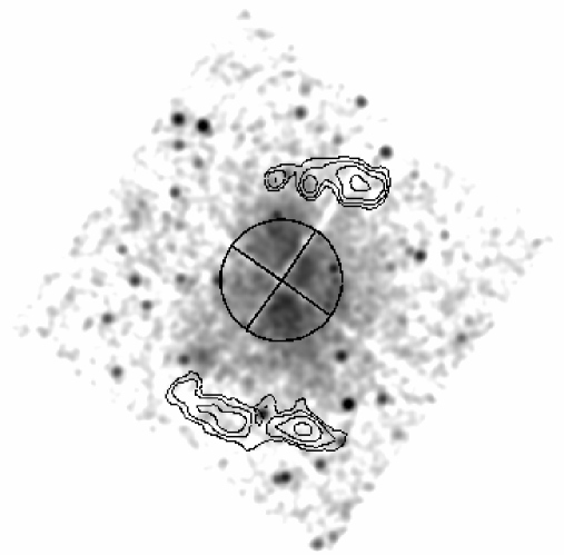
Figure 14: 17^′$\times$17$\mathrm{{}^{\prime}}\;$Chandra X–ray smoothed image (ID 4961) of A1240 in the energy band 0.5–2 keV (North at the top and East to the left). The central circle has a radius of $\sim$2.58$\mathrm{{}^{\prime}}\;$(0.5 Mpc at the cluster redshift, see text). Black contours show the two radio relics.

As for the spectral properties of the cluster X–ray photons, we compute a global estimate of the ICM temperature. The temperature is computed from the X–ray spectrum of the cluster within a circular aperture of $\sim$2.58$\arcmin$ radius (0.5 Mpc at the cluster redshift; see Fig. 14) around the center of the four ACIS chips. Fixing the absorbing galactic hydrogen column density at 1.99$\times$10²⁰ cm^-2, computed from the HI maps by Dickey & Lockman (dic90 (1990)), we fit a Raymond–Smith (ray77 (1977)) spectrum using the CIAO package Sherpa with a $\chi^{2}$ statistics and assuming a metal abundance of 0.3 in solar units. We find a best fitting temperature of $T_{\rm X}=\,$6.0 $\pm\,0.5$ keV.

We then search for temperature gradients by dividing the 0.5 Mpc radius circle in four quadrants (chosen in order to avoid the gaps among the chips), as shown in Fig. 14. As expected for a merging cluster, there is some evidence that the ICM temperature is not homogeneous, with the Western quadrant ($T_{\rm X}$=6.7${}^{+1.9}_{-1.2}$ keV) somewhat hotter than the Northern ($T_{\rm X}$=5.1${}^{+1.0}_{-0.8}$ keV), the Eastern ($T_{\rm X}$=5.2${}^{+1.9}_{-1.2}$ keV) and Southern ($T_{\rm X}$=5.4${}^{+0.9}_{-0.8}$ keV) quadrants. More detailed temperature and metallicity maps would be highly desirable to better describe the properties of the ICM, but the photon statistics is not good enough to this aim. In particular, we do not provide any estimate of the ICM temperature in proximity of the two relics, where the X–ray surface brightness is too low to obtain any reliable measurement (see Fig. 14).

5 Cluster structure: discussion

Both optical and X–ray data indicate that A1240 is a strongly substructured cluster, elongated in the N–S direction, the same of the axis of symmetry of the relics. We also detect two clumps, separated by $1.2$ $h_{70}^{-1}$ Mpc, in the galaxy distribution. These observational features suggest that we are looking at a cluster just forming through the merging of two main subclumps. The difficulty in separating the two subclumps in the velocity space and the small LOS velocity difference of the two BCGs suggest that the axis of the merger lies in the plane of the sky. The evidence of a very disturbed ICM distribution, somewhat displaced from the galaxy distribution, suggests that the merger is seen after the phase of the core passage, as shown by the results of the numerical simulation (e.g., Roettiger et al. roe97 (1997), their Figs. 7–14).

As for the observational cluster structure, A1240 is similar to Abell 3667 (see Roettiger et al. roe99 (1999) and refs. therein) where the optical and X–ray structures are elongated in a direction roughly similar to that of the axis of symmetry of the two radio relics which are separated by $\sim 3-4$ $h_{70}^{-1}$ Mpc. The two intervening galaxy subclumps are separated by $\sim 1$ $h_{70}^{-1}$ Mpc with a small LOS velocity difference $\sim 120$ km s${}^{-1}\;$between the dominant galaxies. Basic observational features of Abell 3667 were explained with the “outgoing merger shocks” model, where shocks provide sites for diffusive shock acceleration of relativistic electrons causing the presence of the radio sources (Roettiger et al. roe99 (1999)).

For A1240 we have detected two galaxy subclumps in the N–S direction, the same direction of the elongation of the X–ray surface brightness and the axis of symmetry of the two radio relics. The values of relevant parameters for the two–clumps system, as deduced from the BCGN and BCGS, are: the relative LOS velocity in the rest–frame, $V_{\rm rf}=390$ km s${}^{-1}\;$, and the projected linear distance between the two clumps, $D=1.2$ $h_{70}^{-1}$ Mpc. The two roughly symmetric relics lie more externally, separated by a projected linear distance $\sim 2$ $h_{70}^{-1}$ Mpc (Bonafede et al. bon09 (2009)).

We now use the above parameters and the mass of the system computed in a range $M_{\rm A1240}=(0.9-1.9)$ $\times 10^{15}\;h_{70}^{-1}\;M_{\odot}\;$to investigate the relative dynamics of A1240N and A1240S. In particular, we use different analytic approaches based on an energy integral formalism in the framework of locally flat spacetime and Newtonian gravity (e.g., Beers et al. bee82 (1982)).

First, we compute the Newtonian criterion for gravitational binding stated in terms of the observables as $V_{\rm r}^{2}D\leq 2GM_{\rm sys}\rm{sin}^{2}\alpha\,\rm{cos}\alpha$, where $\alpha$ is the projection angle between the plane of the sky and the line connecting the centers of the two clumps. The thin curve in Fig. 15 separates the bound and unbound regions according to the Newtonian criterion (above and below the curve, respectively). Considering the lower (upper) limit of $M_{\rm A1240}$, the N+S system is bound between $9\mathrm{{}^{\circ}}$ and $84\mathrm{{}^{\circ}}$ ($6\mathrm{{}^{\circ}}$ and $89\mathrm{{}^{\circ}}$); the corresponding probability, computed considering the solid angles (i.e., $\int^{\alpha 2}_{\alpha 1}{\rm cos}\,\alpha\,d\alpha$), is 84% (89%).

Then, we apply the analytical two–body model introduced by Beers et al. (bee82 (1982)) and Thompson (tho82 (1982); see also Lubin et al. lub98 (1998) for a more recent application). This model assumes radial orbits for the clumps with no shear or net rotation of the system. According to the boundary conditions usually considered, the clumps are assumed to start their evolution at time $t_{0}=0$ with separation $d_{0}=0$, and now moving apart or coming together for the first time in their history.

In the case of A1240N+A1240S system, where the first core passage has likely already occurred, we assume that the time $t_{0}=0$ with separation $d_{0}=0$ is the time of their core crossing and that we are looking at the cluster a time $t$ after. To obtain an estimate of $t$ we use the Mach number of the shock ${\cal M}\sim 3$ as recovered by Bonafede et al. (bon09 (2009)) from the radio spectral index. The Mach number is defined as ${\cal M}={\rm v}_{\rm s}/c_{\rm s}$, where ${\rm v}_{\rm s}$ is the velocity of the shock and $c_{\rm s}$ in the sound speed in the pre–shock gas (see e.g., Sarazin sar02 (2002) for a review). The value of $c_{\rm s}$, obtained from our estimate of $T_{\rm X}$, i.e. $c_{\rm s}\sim 995$ km s^-1, leads to a value of ${\rm v}_{\rm s}\sim 3\times 10^{3}$ km s^-1. Assuming the shock velocity as a constant, the shock covered a $\sim 1$ $h_{70}^{-1}$ Mpc scale (i.e. the distance of the relics from the cluster center) in a time of $\sim 0.3$ Gyrs. We assume this time as our estimate of $t$. Although the velocity of the shock is not constant, recent studies based on numerical simulations show how the variation of ${\rm v}_{\rm s}$ is much smaller than the variation of the relative velocity of the subclumps identified with their dark matter components (see Fig. 4 of Springel & Farrar spr07 (2007); see Fig. 14 of Mastropietro & Burkert mas08 (2008)), thus our rough estimate of $t$ is acceptable at the first order of approximation.

The bimodal model solution gives the total system mass $M_{\rm sys}$ as a function of $\alpha$ (e.g., Gregory & Thompson gre84 (1984)). Figure 15 compares the bimodal–model solutions with the observed mass of the system. The present solutions span the bound outgoing solutions (i.e. expanding), BO; the bound incoming solutions (i.e. collapsing), BI_a and BI_b; and the unbound outgoing solutions, UO. For the incoming case there are two solutions because of the ambiguity in the projection angle $\alpha$. Both the BO and UO solutions are, in principle, consistent with the observed mass range. However, the BO solution is the more likely since the probability associated to the BO solution is much higher than that associated to the UO solution. In fact, we obtain that P(BO) and P(UO) are $92\%$ and $8\%$, respectively, where these probabilities are computed considering the solid angles (see above) and assuming that the region of $M_{\rm sys}$ values is equally probable for individual solutions (see e.g. Barrena et al. 2007b ). As for the projection angle we estimate a value of $\alpha\sim 10$^∘. This small angle means that the real spatial distance between A1240 subclumps is similar to the projected one while the real, i.e. deprojected, velocity difference is $V_{\rm rf}\sim 2000$ km s^-1, a quite reasonable value during cluster mergers (see, e.g. Springel & Farrar spr07 (2007) and refs. therein). Notice that the relative velocity between galaxy clumps is smaller than the shock velocity, i.e. the regime is not stationary, but this is expected when comparing shock and collisionless components in numerical simulations (Springel & Farrar spr07 (2007); Mastropietro & Burkert mas08 (2008)).

Figure 15: System mass vs. projection angle for bound and unbound solutions (thick solid and thick dashed curves, respectively) of the two–body model applied to A1240N and A1240S subsystems. Labels BI_a and BI_b indicate the bound and incoming, i.e. collapsing solutions (thick solid curve). Label BO indicates the bound outgoing, i.e. expanding solutions (thick solid curve). Label UO indicates the unbound outgoing solutions (thick dashed curve). The horizontal lines give the range of observational values of the mass system. The thin dashed curve separates bound and unbound regions according to the Newtonian criterion (above and below the thin dashed curve, respectively).

Since the merger of A1240 clumps occurred largely in the plane of the sky, this likely explains the similarity between the observational features of A1240 and Abell 3667. However, the case of A1240 is made more complex by the presence of A1237.

We investigate the relative dynamics of A1237 and A1240 with the same approach described above. The values of the relevant observable quantities for the two–clumps system are based on Table 2, i.e. LOS $V_{\rm rf}=320$ km s${}^{-1}\;$and $D=2.7$ $h_{70}^{-1}$ Mpc. For the mass of the system we use the mass range computed in Sect. 3.6, $M_{\rm A1237+A1240}=(15-25)$ $\times 10^{15}\;h_{70}^{-1}\;M_{\odot}$. The Newtonian criterion for gravitational binding leads to a system bound between $8\mathrm{{}^{\circ}}$ and $89\mathrm{{}^{\circ}}$ ($7\mathrm{{}^{\circ}}$ and $89\mathrm{{}^{\circ}}$); the corresponding probability, computed considering the solid angles (i.e., $\int^{89}_{6}{\rm cos}\,\alpha\,d\alpha$), is $87\%$ ($89\%$).

In the case of A1237 and A1240 we have no evidence of a previous merger since the gas distribution of A1240 (although very complex) does not show evidence of a peculiar displacement in direction of A1237. Therefore we assume that we are looking at A1237 and A1240 before their encounter. X–ray observations of A1237 would be useful to confirm this hypothesis. Under our assumption we can use the standard version of the analytical two–body model to study the A1237+A1240 system, where the clumps are assumed to start their evolution at time $t_{0}=0$ with separation $d_{0}=0$, and are moving apart or coming together for the first time in their history. We are looking at the system at the time of $t=11.090$ Gyrs, i.e. the age of the Universe at the system redshift. The solutions consistent with the observed mass span these cases: the bound and present incoming solution (i.e. collapsing), BI_a and BI_b, and the bound–outgoing solution, BO (see Fig. 16). The associated probabilities are $61\%$, $31\%$ and $8\%$, for BI_a, BI_b and BO respectively. The most probable solution is also the most interesting one since the BI_a solution gives the same value of $\alpha\sim 10$^∘already found for the A1240N+S merger. In this case, the direction of the clump velocities are consistent, too: at the present time A1240N has already crossed A1240S, being now in front of A1240S and moving outgoing; A1237 is lying behind A1240 and is infalling onto it along almost the same N–S direction.

Figure 16: System mass vs. projection angle for bound and unbound solutions (solid and dashed curves, respectively) of the two–body model applied to A1237 and A1240 systems.

6 Conclusions

Our results strongly support the conclusion of Bonafede et al. (bon09 (2009)), based on radio data, in favor of the “outgoing merger shocks” model for the double relics of A1240. In fact, we detect the intervening merging subclumps and recover an acceptable model for the internal cluster dynamics. Moreover, our results also suggest that we are looking at the cluster accretion along a large scale structure filament.

Our analysis shows how powerful is the study of the internal cluster dynamics through the analysis of kinematics of cluster galaxies. Other insights into A1240 might be recovered from a better knowledge of galaxy properties, e.g. spectral signatures of past activity which could be useful to determine the relevant time–scales (see e.g., Ferrari et al. fer03 (2003); Boschin et al. bos04 (2004)) and from deeper X–ray observations (see, e.g Vikhlinin et al. vik01 (2001) for the discover of a “cold front” in Abell 3667). Finally, we point out that A1240, with its displacement between collisional (gas) and collisionless components (galaxies), is an excellent candidate to study the properties of the dark matter, in particular its collisional cross section, as already performed in other merging clusters (Markevitch et al. mar04 (2004); Bradǎc et al. bra08 (2008)).

- (1) Abell, G. O., Corwin, H. G. Jr., & Olowin, R. P. 1989, ApJS, 70, 1
- (2) Ashman, K. M., Bird, C. M., & Zepf, S. E. 1994, AJ, 108, 2348
- (3) Bagchi, J., Durret, F., Lima Neto, G. B., & Paul, S. 2006, Science, 314, 791
- (4) Bardelli, S., Zucca, E., Vettolani, G., et al. 1994, MNRAS, 267, 665
- (5) Barrena, R., Boschin, W., Girardi, M., & Spolaor, M. 2007a, A&A, 467, 37
- (6) Barrena, R., Boschin, W., Girardi, M., & Spolaor, M. 2007b, A&A, 469, 861
- (7) Beers, T. C., Flynn, K., & Gebhardt, K. 1990, AJ, 100, 32
- (8) Beers, T. C., Forman, W., Huchra, J. P., Jones, C., & Gebhardt, K. 1991, AJ, 102, 1581
- (9) Beers, T. C., & Geller, M. J. 1983, ApJ, 274, 491
- (10) Beers, T. C., Geller, M. J., & Huchra, J. P. 1982, ApJ, 257, 23
- (11) Bertin, E., & Arnouts, S. 1996, A&AS, 117, 393
- (12) Bird, C. M., & Beers, T. C. 1993, AJ, 105, 1596
- (13) Bonafede, A., Giovannini, G., Feretti, L., Govoni, F., & Murgia M. 2009, A&A, 494, 429
- (14) Boschin, W., Barrena, R., & Girardi, M. 2009, A&A, 495, 15
- (15) Boschin, W., Barrena, R., Girardi, M., & Spolaor, M. 2008, A&A, 487, 33
- (16) Boschin, W., Girardi, M., Barrena, R., et al. 2004, A&A, 416, 839
- (17) Boschin, W., Girardi, M., Spolaor, M., & Barrena, R. 2006, A&A, 449, 461
- (18) Bradǎc, M., Allen, S. W., Treu, T., et al. 2008, ApJ, 687, 959
- (19) Buote, D. A. 2002, in “Merging Processes in Galaxy Clusters”, eds. L. Feretti, I. M. Gioia, & G. Giovannini (The Netherlands, Kluwer Ac. Pub.): Optical Analysis of Cluster Mergers
- (20) Burstein, D., & Heiles, C. 1982, AJ, 87, 1165
- (21) Carlberg, R. G., Yee, H. K. C., & Ellingson, E. 1997, ApJ, 478, 462
- (22) Cassano, R., & Brunetti, G. 2005, MNRAS, 357, 1313
- (23) Cousins, A. W. J., 1976, Mem. R. Astr. Soc, 81, 25
- (24) Danese, L., De Zotti, C., & di Tullio, G. 1980, A&A, 82, 322
- (25) David, L. P., Forman, W., & Jones, C. 1999, ApJ, 519, 533
- (26) Dickey, J. M., & Lockman, F. J. 1990, ARA&A, 28, 215
- (27) Dressler, A., & Shectman, S. A. 1988, AJ, 95, 985
- (28) Ebeling, H., Voges, W., Böhringer, H., et al. 1996, MNRAS, 281, 799
- (29) Ellingson, E., & Yee, H. K. C. 1994, ApJS, 92, 33
- (30) Ensslin, T. A., Biermann, P. L., Klein, U., & Kohle, S. 1998, A&A, 332, 395
- (31) Ensslin, T. A., & Gopal–Krishna 2001, A&A, 366, 26
- (32) Fadda, D., Girardi, M., Giuricin, G., Mardirossian, F., & Mezzetti, M. 1996, ApJ, 473, 670
- (33) Fasano, G., & Franceschini, A. 1987, MNRAS, 225, 155
- (34) Feretti, L. 2008, Mem. SAIt, 79, 176
- (35) Feretti, L. 2006, Proceedings of the XLIst Rencontres de Moriond, XXVIth Astrophysics Moriond Meeting: ”From dark halos to light”, L.Tresse, S. Maurogordato and J. Tran Thanh Van, Eds, e-print astro-ph/0612185
- (36) Feretti, L. 1999, MPE Report No. 271
- (37) Feretti, L. 2002a, The Universe at Low Radio Frequencies, Proceedings of IAU Symposium 199, held 30 Nov – 4 Dec 1999, Pune, India. Edited by A. Pramesh Rao, G. Swarup, and Gopal–Krishna, 2002., p.133
- (38) Feretti, L. 2005a, X–Ray and Radio Connections (eds. L. O. Sjouwerman and K. K. Dyer). Published electronically by NRAO, http://www.aoc.nrao.edu/events/xraydio. Held 3–6 February 2004 in Santa Fe, New Mexico, USA
- (39) Feretti, L., Gioia I. M., and Giovannini G. eds., 2002b, Astrophysics and Space Science Library, vol. 272 “Merging Processes in Galaxy Clusters”, Kluwer Academic Publisher, The Netherlands
- (40) Feretti, L., Schuecker, P., Böehringer, H., Govoni, F., & Giovannini, G. 2005b, A&A, 444, 157
- (41) Ferrari, C., Govoni, F., Schindler, S., Bykov, A. M., & Rephaeli, Y. 2008, Space Sci. Rev., 134, 93
- (42) Ferrari, C., Maurogordato, S., Cappi, A., & Benoist C. 2003, A&A, 399, 813
- (43) Flores, R. A., Quintana, H., & Way, M. J. 2000, ApJ, 532, 206
- (44) Gal, R. R., de Carvalho, R. R., Lopes, P. A. A., et al. 2003, AJ, 125, 2064
- (45) Giovannini, G., & Feretti, L. 2002, in “Merging Processes in Galaxy Clusters”, eds. L. Feretti, I. M. Gioia, & G. Giovannini (The Netherlands, Kluwer Ac. Pub.): Diffuse Radio Sources and Cluster Mergers
- (46) Giovannini, G., Tordi, M., & Feretti, L. 1999, New Astronomy, 4, 141
- (47) Girardi, M., Barrena, R., and Boschin, W. 2007, Contribution to “Tracing Cosmic Evolution with Clusters of Galaxies: Six Years Later” conference – http://www.si.inaf.it/sesto2007/contributions/Girardi.pdf
- (48) Girardi, M., & Biviano, A. 2002, in “Merging Processes in Galaxy Clusters”, eds. L. Feretti, I. M. Gioia, & G. Giovannini (The Netherlands, Kluwer Ac. Pub.): Optical Analysis of Cluster Mergers
- (49) Girardi, M., Biviano, A., Giuricin, G., Mardirossian, F., & Mezzetti, M. 1995, ApJ, 438, 527
- (50) Girardi, M., Escalera, E., Fadda, D., et al. 1997, ApJ, 482, 11
- (51) Girardi, M., Fadda, D., Giuricin, G. et al. 1996, ApJ, 457, 61
- (52) Girardi, M., Giuricin, G., Mardirossian, F., Mezzetti, M., & Boschin, W. 1998, ApJ, 505, 74
- (53) Girardi, M., & Mezzetti, M. 2001, ApJ, 548, 79
- (54) Goto, T., Sekiguchi, M., Nichol, R. C., et al. 2002, AJ, 123, 1807
- (55) Gregory, S. A., & Thompson, L. A. 1984, ApJ, 286, 422
- (56) Gullixson, C. A. 1992, in “Astronomical CCD Observing and Reduction techniques” (ed. S. B. Howell), ASP Conf. Ser., 23, 130
- (57) Hoeft, M., Brüggen, M., & Yepes, G. 2004, MNRAS, 347, 389
- (58) Johnson, H. L., & Morgan, W. W. 1953, ApJ, 117, 313
- (59) Kempner, J. C., Blanton, E. L., Clarke, T. E. et al. 2003, Proceedings of “The Riddle of Cooling Flows in Galaxies and Clusters of Galaxies”, eds. T. H. Reiprich, J. C. Kempner, & N. Soker, e-print astro-ph/0310263
- (60) Kempner, J. C., & Sarazin, C. L. 2001, ApJ, 548, 639
- (61) Kennicutt, R. C. 1992, ApJS, 79, 225
- (62) Koester, B. P., McKay, T. A., Annis, J., et al. 2007, ApJ, 660, 239
- (63) Limber, D. N., & Mathews, W. G. 1960, ApJ, 132, 286
- (64) López–Cruz, O., Barkhouse, W. A., & Yee, H. K. C. 2004, ApJ, 614, 679
- (65) Lubin, L. M., Postman, M., & Oke, J. B. 1998, AJ, 116, 643
- (66) Malumuth, E. M., Kriss, G. A., Dixon, W. Van Dyke, Ferguson, H. C., & Ritchie, C. 1992, AJ, 104, 495
- (67) Markevitch, M., Gonzalez, A. H., Clowe, D., et al. 2004, ApJ, 606, 819
- (68) Mastropietro, C., & Burkert, A. 2008, MNRAS, 389, 967
- (69) Mazure, A., Proust, D., Mathez, G., & Mellier, Y. 1988, A&AS, 76, 339
- (70) Pisani, A. 1993, MNRAS, 265, 706
- (71) Pisani, A. 1996, MNRAS, 278, 697
- (72) Poggianti, B. M. 1997, A&AS, 122, 399
- (73) Press, W. H., Teukolsky, S. A., Vetterling, W. T., & Flannery, B. P. 1992, in Numerical Recipes (Second Edition), (Cambridge University Press)
- (74) Quintana, H., Carrasco, E. R., & Reisenegger, A. 2000, AJ, 120, 511
- (75) Quintana, H., Ramírez, A., & Way, M. J. 1996, AJ, 112, 360
- (76) Raymond, J. C., & Smith, B. W. 1977, ApJS, 35, 419
- (77) Roettiger, K., Burns, J. O., & Stone, J. M. 1999, ApJ, 518, 603
- (78) Roettiger, K., Loken, C., & Burns, J. O. 1997, ApJS, 109, 307
- (79) Röttgering, H. J. A., Wieringa, M. H., Hunstead, R. W., & Ekers, R. D. 1997, MNRAS, 290, 577
- (80) Sarazin, C. L. 2002, in “Merging Processes in Galaxy Clusters”, eds. L. Feretti, I. M. Gioia, & G. Giovannini (The Netherlands, Kluwer Ac. Pub.): The Physics of Cluster Mergers
- (81) Springel, V., & Farrar, G. R. 2007, MNRAS, 380, 911
- (82) The, L. S., & White, S. D. M. 1986, AJ, 92, 1248
- (83) Thompson, L. A. 1982, in IAU Symposium 104, Early Evolution of the Universe and the Present Structure, eds. G.O. Abell and G. Chincarini (Dordrecht: Reidel)
- (84) Tonry, J., & Davis, M. 1979, ApJ, 84, 1511
- (85) Venturi, T., Giacintucci, S., Brunetti, G., et al. 2007, A&A, 4363, 937
- (86) Vikhlinin, A., Markevitch, M., & Murray, S. S. 2001, ApJ, 551, 160
- (87) Visvanathan, N., & Sandage, A. 1977, ApJ, 216, 214
- (88) Wainer, H., & Schacht, S. 1978, Psychometrika, 43, 203