Piecewise Parabolic Method on a Local Stencil for Magnetized Supersonic Turbulence Simulation

Abstract

Stable, accurate, divergence-free simulation of magnetized supersonic turbulence is a severe test of numerical MHD schemes and has been surprisingly difficult to achieve due to the range of flow conditions present. Here we present a new, higher order-accurate, low dissipation numerical method which requires no additional dissipation or local ”fixes” for stable execution. We describe PPML, a local stencil variant of the popular PPM algorithm for solving the equations of compressible ideal magnetohydrodynamics. The principal difference between PPML and PPM is that cell interface states are evolved rather that reconstructed at every timestep, resulting in a compact stencil. Interface states are evolved using Riemann invariants containing all transverse derivative information. The conservation laws are updated in an unsplit fashion, making the scheme fully multidimensional. Divergence-free evolution of the magnetic field is maintained using the higher order-accurate constrained transport technique of Gardiner and Stone. The accuracy and stability of the scheme is documented against a bank of standard test problems drawn from the literature. The method is applied to numerical simulation of supersonic MHD turbulence, which is important for many problems in astrophysics, including star formation in dark molecular clouds. PPML accurately reproduces in three-dimensions a transition to turbulence in highly compressible isothermal gas in a molecular cloud model. The low dissipation and wide spectral bandwidth of this method make it an ideal candidate for direct turbulence simulations.

1 Introduction

Piecewise Parabolic Method on a Local Stencil (PPML) [1, 2] is a new numerical scheme developed for solving multidimensional compressible Euler (HD) and ideal magnetohydrodynamic (MHD) equations. The method is based on a piecewise parabolic approximation of variables inside individual grid cells. It is third order-accurate in space and it implies second order temporal accuracy. This method is an improvement over the popular PPM introduced by Colella and Woodward [3, 4] for nonmagnetized flows with strong shocks and extended by Dai and Woodward to compressible ideal magnetohydrodynamics [5]. PPM has been widely used in computational practice ever since, and versions of the PPM gas dynamics scheme have been incorporated into a number of codes for astrophysical applications [6].

The main new feature of PPML is the procedure for calculating interface values between adjacent cells. Instead of an interpolation procedure used in the original PPM formulation, which employs a four-point stencil, PPML relies on the information preserved from a previous time step. The required values are obtained via Riemann invariants transferred along the characteristic curves of the equations to cell boundaries using an approximate parabolic solution within a cell [7, 8, 9, 10, 11]. To preserve the order of the scheme at local extrema, a monotonicity constraint is applied to these interface values [12, 13, 14, 15]. In a multidimensional case a monotonicity preserving method from [16] is additionally applied. The scheme is multidimensional as it keeps terms containing derivatives with respect to the tangential directions in the equations for wave amplitudes. This approach provides the left and right states for the Riemann problem based on multidimensional reconstruction. For the ideal MHD case in three dimensions, a zero-divergence constraint on the magnetic field is enforced by the use of the Stokes theorem (the so-called constrained transport approach [17]). An updated component of the electric field at a cell boundary is calculated by averaging the quantities obtained from given components of flux-vectors, taking into account a value of the electric field gradient and the information about the sign of the tangential velocity at that boundary [18].

PPML has been tested on a number HD and MHD problems that demonstrated the ability of the method to resolve discontinuous solutions without adding excessive dissipation. PPML provides a very accurate treatment of strong discontinuities, minimizes numerical dissipation of the kinetic and magnetic energy, and substantially improves the spectral bandwidth for compressible turbulence models compared to its predecessors [19].

In this paper we present a comprehensive description of the numerical method for 3D MHD simulations as well as results of numerical tests. The method has been substantially improved and remastered compared to its previous version presented in [1, 2]. The new PPML features in this paper include: (i) an improved approach to maintaining zero divergence for the magnetic field following [18], see Section 5; (ii) a monotonicity constraint proposed by Rider et al. [14], as described in Section 6; (iii) an extended suite of test problems that includes a comparison with the FLASH3 MHD solver, see Section 8; Finally, in Section 9 we illustrate the performance of PPML on a three-dimensional problem of highly compressible weakly magnetized forced turbulence with a sonic Mach number of 10. The problem of supersonic, super-Alfvénic turbulence with an isothermal equation of state proved to be a challenging regime for numerical modeling due to the presence of strong rarefactions and very high density contrasts in the flow. PPML scheme is perfectly stable numerically on problems of this sort. We also briefly discuss the effects of the weak magnetic field on the spectral properties of MHD turbulence and obtain good correspondence between our numerical results and observed characteristics of supersonic turbulence in star forming molecular clouds.

2 PPML description

Let us consider a homogeneous one-dimensional grid with the spacing $h$ and a function $q(x,t_{0})\equiv q_{0}(x)$ defined on this grid at $t=t_{0}$. It is assumed that the function $q_{0}(x)$ can be approximated by a parabola inside every grid cell (Fig. 1):

Figure 1: Approximation of $q(x)$ inside a cell.

$$q_{0}(x)=q_{i}^{L}+\xi\left(\Delta q_{i}+q_{i}^{(6)}(1-\xi)\right),$$ (1)

where

$$\xi=\left(x-x_{i-1/2}\right)h^{-1},\quad\Delta q_{i}=q_{i}^{R}-q_{i}^{L},$$

$$q_{i}^{(6)}=6\left(q_{i}-1/2\left(q_{i}^{L}+q_{i}^{R}\right)\right).$$

Function $q_{i}$ satisfies a condition

$$q_{i}=h^{-1}\int\limits_{x_{i-1/2}}^{x_{i+1/2}}q_{0}(x)\,dx.$$

Let us consider a linear advection equation

$$\frac{\partial q(x,t)}{\partial t}+\frac{\partial F(x,t)}{\partial x}=0,$$ (2)

where $F(x,t)=a\,q(x,t)$ and find its solution for the moment $t=t_{0}+\tau$. On a discrete grid we have a number of local Riemann problems which lead to some average states $q^{*}(x_{i+1/2},t)$ on every interface $x_{i+1/2}$ between the adjacent cells. The equation (2) has only one characteristic defined by $dx/dt=a$. To find a value $q_{i+1/2}$, for example, on the right boundary of a cell number $i$ at the time step $t=t_{0}+\tau$, we suggest to move along the characteristic line from the point $x_{i+1/2}$ back to the moment $t=t_{0}$ and use a value from some point on a previous parabola (Fig. 2).

Then for $a>0$ we have

$$q_{i+1/2}(t_{0}+\tau)\equiv q_{i}^{\,R}(t_{0}+\tau)=q_{i}^{\,L}+\xi\left(\Delta q_{i}+q_{i}^{(6)}(1-\xi)\right),$$ (3)

where

$$\xi=\left(x-x_{i-1/2}\right)h^{-1}=\left(h-a\tau\right)h^{-1}=1-a\tau h^{-1}.$$ (4)

All the values in the rhs of (3) must be taken from a previous time step $t=t_{0}$. For $a<0$ a value $q_{i+1/2}$ is defined by a parabola in the cell number $i+1$:

$$q_{i+1/2}(t_{0}+\tau)\equiv q_{i+1}^{\,L}(t_{0}+\tau)=q_{i+1}^{\,L}+\xi\left(\Delta q_{i+1}+q_{i+1}^{(6)}(1-\xi)\right),$$

where $\xi=-a\tau h^{-1}$.

Figure 2: A characteristic inside a grid cell ($a>0$).

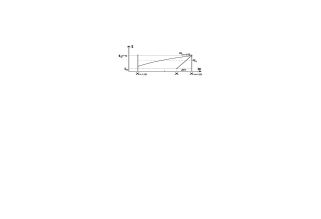
In monotonic regions, where $q_{i+1/2}\in\left[q_{i}\ldots q_{i+1}\right]$, it is assumed that $q_{i}^{\,R}=q_{i+1}^{\,L}=q_{i+1/2}$ and $q_{i}^{\,L}=q_{i-1}^{\,R}=q_{i-1/2}$. In non-monotonic regions we must redefine $q_{i}^{\,L}$ and $q_{i}^{\,R}$. If $q_{i}$ is a local maximum or minimum, the interpolation function (1) must be constant, i.e. $q_{i}^{\,L}=q_{i}^{\,R}=q_{i}$. If $q_{i}$ is too close to $q_{i}^{\,L}$ or $q_{i}^{\,R}$, the parabola (1) can have an extremum inside the grid cell (it happens when $|\Delta q_{i}|<|q_{i}^{(6)}|$). In this case we must move this extremum to the boundary of the cell. These conditions can be written as

$$q_{i}^{\,L}=q_{i},\quad q_{i}^{\,R}=q_{i},\quad\mbox{if}\;\left(q_{i}^{\,L}-q_{i}\right)\left(q_{i}-q_{i}^{\,R}\right)\leq 0$$ (5)

and

$$\begin{array}[]{l}q_{i}^{\,L}=3q_{i}-2q_{i}^{\,R},\quad\mbox{if}\;\;\Delta q_{i}\cdot q_{i}^{(6)}>\left(\Delta q_{i}\right)^{2},\\ q_{i}^{\,R}=3q_{i}-2q_{i}^{\,L},\quad\mbox{if}\;\;\Delta q_{i}\cdot q_{i}^{(6)}<-\left(\Delta q_{i}\right)^{2}.\\ \end{array}$$ (6)

If we know the function $q(x)$, we can compute its average for the interval

$\left[x_{i+1/2}-y\ldots x_{i+1/2}\right]$ (for $y>0$):

$$\overline{q}_{i+1/2}^{\,L}(y)=y^{-1}\int\limits_{x_{i+1/2}-y}^{x_{i+1/2}}q(x)\,dx=q_{i}^{\,R}-1/2\,y\,h^{-1}\left[\Delta q_{i}-\left(1-2/3\,y\,h^{-1}\right)q_{i}^{(6)}\right].$$ (7)

For $a>0$, the solution of (2) at time $t=t_{0}+\tau$ can be found by averaging over the interval $\left[x_{i+1/2}-a\tau\ldots x_{i+1/2}\right]$, i.e. $q^{*}(x_{i+1/2},t_{0}+\tau)\equiv q_{i+1/2}^{\,L}=\overline{q}_{i+1/2}^{\,L}(a\tau)$. For $a<0$ the zone of influence is $\left[x_{i+1/2}\ldots x_{i+1/2}+a\tau\right]$. In this case $q^{*}(x_{i+1/2},t_{0}+\tau)\equiv q_{i+1/2}^{\,R}=\overline{q}_{i+1/2}^{\,R}(-a\tau)$, where

$$\overline{q}_{i+1/2}^{\,R}(y)=y^{-1}\int\limits_{x_{i+1/2}}^{x_{i+1/2}+y}q(x)\,dx\\ =q_{i+1}^{\,L}+1/2\,y\,h^{-1}\left[\Delta q_{i+1}+\left(1-2/3\,y\,h^{-1}\right)q_{i+1}^{(6)}\right],\quad y>0.$$ (8)

The flux on the interface can be computed as

$$F_{i+1/2}=a^{+}q_{i+1/2}^{\,L}+a^{-}q_{i+1/2}^{\,R},$$ (9)

where $a^{+}=\max(a,0)=\left(a+|a|\right)/2$, $a^{-}=\min(a,0)=\left(a-|a|\right)/2$. We can use an arbitrary value for $q_{i+1/2}^{\,L}$ if $a<0$, and for $q_{i+1/2}^{\,R}$ if $a>0$.

3 The governing equations

Let us consider the ideal MHD equations in 3D in the following form:

$$\partial_{t}{\bf U}+\partial_{x}{\bf F}+\partial_{y}{\bf G}+\partial_{z}{\bf H}=0.$$ (10)

Here ${\bf U}$ is a vector of eight conservative variables, ${\bf F}$, ${\bf G}$ and ${\bf H}$ are the fluxes:

$${\bf U}=\left(\rho,\rho\,u,\rho\,v,\rho\,w,B_{x},B_{y},B_{z},E\right)^{T},$$ (11)

$${\bf F}=\left(\rho\,u,\rho\,u^{2}+\overline{p}-B_{x}^{2},\rho uv-B_{x}B_{y},\rho uw-B_{x}B_{z},0,\right.\\ \bigl{.}uB_{y}-vB_{x},uB_{z}-wB_{x},u(E+\overline{p})-B_{x}(uB_{x}+vB_{y}+wB_{z})\bigr{)}^{T},$$ (12)

$${\bf G}=\left(\rho\,v,\rho uv-B_{x}B_{y},\rho\,v^{2}+\overline{p}-B_{y}^{2},\rho vw-B_{y}B_{z},vB_{x}-uB_{y},\right.\\ \bigl{.}0,vB_{z}-wB_{y},v(E+\overline{p})-B_{y}(uB_{x}+vB_{y}+wB_{z})\bigr{)}^{T},$$ (13)

$${\bf H}=\left(\rho\,w,\rho uw-B_{x}B_{z},\rho vw-B_{y}B_{z},\rho\,w^{2}+\overline{p}-B_{z}^{2},wB_{x}-uB_{z},\right.\\ \bigl{.}wB_{y}-vB_{z},0,w(E+\overline{p})-B_{z}(uB_{x}+vB_{y}+wB_{z})\bigr{)}^{T},$$ (14)

where $\rho$ is the density; $u$, $v$ and $w$ are the velocity components; $B_{x}$, $B_{y}$ and $B_{z}$ are the magnetic field components; $E$ is the total energy and $\overline{p}$ is the total pressure:

$$\overline{p}=p+\frac{\bf BB}{2}.$$

We have included the factor $1/\sqrt{4\pi}$ in the definition of ${\bf B}$. An equation for the total energy and an ideal gas equation of state are

$$E=\rho\,\varepsilon+\frac{\rho{\bf vv}}{2}+\frac{{\bf BB}}{2},$$

$$p=(\gamma-1)\,\rho\,\varepsilon,$$

where $\gamma$ - the adiabatic index, $\varepsilon$ - the specific internal energy. If we denote

$$(b_{x},b_{y},b_{z})=\frac{1}{\sqrt{\rho}}\left(B_{x},B_{y},B_{z}\right),\quad b^{2}=b_{x}^{2}+b_{y}^{2}+b_{z}^{2},$$

we can write the sound velocity $c$, Alfvén velocity $c_{a}$, the fast and the slow magneto-acoustic velocities $c_{f,\,s}$ as

$$c=\sqrt{\frac{\gamma p}{\rho}},$$

$$c_{a}=|b_{x}|,$$

$$c_{f,\,s}=\left[\frac{1}{2}\left(c^{\,2}+b^{\,2}\right)\pm\frac{1}{2}\sqrt{\left(c^{\,2}+b^{\,2}\right)^{\,2}-4c^{\,2}b_{x}^{\,2}}\right]^{1/2}.$$

We will also deal with a non-conservative form of the MHD equations:

$$\partial_{t}{\bf V}+A\,\partial_{x}{\bf V}+B\,\partial_{y}{\bf V}+C\,\partial_{y}{\bf V}=0,$$ (15)

where

$${\bf V}=\left(\rho,u,v,w,B_{x},B_{y},B_{z},p\,\right)^{T}.$$ (16)

The matrices $A$, $B$ and $C$ can be computed using Jacobians of (10) and a transition matrix

$$M=\frac{\partial{\,\bf U}}{\partial{\,\bf V}}.$$

For example, the Jacoby matrix $A$ is

$$A=M^{-1}\,\frac{\partial{\,\bf F}}{\partial{\,\bf U}}\,M=\left(\begin{array}[]{cccccccc}u&\rho&0&0&0&0&0&0\\ 0&u&0&0&0&B_{y}/\rho&B_{z}/\rho&1/\rho\\ 0&0&u&0&0&-B_{x}/\rho&0&0\\ 0&0&0&u&0&0&-B_{x}/\rho&0\\ 0&0&0&0&u&0&0&0\\ 0&B_{y}&-B_{x}&0&0&u&0&0\\ 0&B_{z}&0&-B_{x}&0&0&u&0\\ 0&\gamma p&0&0&0&0&0&u\\ \end{array}\right).$$ (17)

The corresponding eigenvalues are

$$\lambda^{\,1,\,8}_{\,x}=u\pm c_{f},\quad\lambda^{\,2,\,7}_{\,x}=u\pm c_{a},\quad\lambda^{\,3,\,6}_{\,x}=u\pm c_{s},\quad\lambda^{\,4,\,5}_{\,x}=u.$$

$\lambda^{\,1,\,8}_{\,x}$ represent a pair of fast magneto-acoustic waves, $\lambda^{\,2,\,7}_{\,x}$ – a pair of Alfvén waves, $\lambda^{\,3,\,6}_{\,x}$ – a pair of slow magneto-acoustic waves, $\lambda^{\,4}_{\,x}$ – an entropy wave, $\lambda^{\,5}_{\,x}$ – a magnetic-flux wave. The eigenvectors of the Jacobians could have singularities at the points of degeneracy of the eigenvalues since the MHD equations are nonstrictly hyperbolic. To avoid those, Brio and Wu [20] suggested a scaled version of the eigenvectors that comes from defining

$$(\beta_{y},\beta_{z})=\left\{\begin{aligned} \frac{(B_{y},B_{z})}{\sqrt{B_{y}^{\,2}+B_{z}^{\,2}}}\quad\mbox{if}\;B_{y}^{\,2}+B_{z}^{\,2}\neq 0,\\ \left(\frac{1}{\sqrt{2}},\frac{1}{\sqrt{2}}\right)\;\mbox{otherwise},\\ \end{aligned}\right.$$

$$(\alpha_{f},\alpha_{s})=\left\{\begin{aligned} \frac{\left(\sqrt{\vphantom{c_{f}^{2}}c^{\,2}-c_{s}^{\,2}},\sqrt{c_{f}^{\,2}-c^{\,2}}\right)}{\sqrt{c_{f}^{\,2}-c_{s}^{\,2}}}\quad\mbox{if}\;B_{y}^{\,2}+B_{z}^{\,2}\neq 0\;\mbox{or}\;\gamma p\neq B_{x}^{\,2},\\ \left(\frac{1}{\sqrt{2}},\frac{1}{\sqrt{2}}\right)\;\mbox{otherwise.}\\ \end{aligned}\right.$$

Thus the left and the right eigenvectors are

$${\bf l}^{\,1,\,8}_{\,x}=\left(\vphantom{\frac{1}{2}}0,\pm\frac{\alpha_{f}\,c_{f}}{2c^{\,2}},\mp\frac{\alpha_{s}}{2c^{\,2}}\,c_{s}\,\beta_{y}\,{\rm sgn}B_{x},\mp\frac{\alpha_{s}}{2c^{\,2}}\,c_{s}\,\beta_{z}\,{\rm sgn}B_{x},\right.\\ \left.0,\frac{\alpha_{s}}{2\sqrt{\rho}\,c}\,\beta_{y},\frac{\alpha_{s}}{2\sqrt{\rho}\,c}\,\beta_{z},\frac{\alpha_{f}}{2\rho\,c^{\,2}}\vphantom{\frac{1}{2}}\right),$$

$${\bf r}^{\,1,\,8}_{\,x}=\left(\vphantom{A^{A^{A}}}\rho\,\alpha_{f},\pm\alpha_{f}\,c_{f},\mp\alpha_{s}\,c_{s}\,\beta_{y}\,{\rm sgn}B_{x},\mp\alpha_{s}\,c_{s}\,\beta_{z}\,{\rm sgn}B_{x},\right.\\ \left.0,\alpha_{s}\sqrt{\rho}\,c\,\beta_{y},\alpha_{s}\sqrt{\rho}\,c\,\beta_{z},\alpha_{f}\gamma\,p\vphantom{A^{A^{A}}}\right)^{T},$$

$${\bf l}^{\,2,\,7}_{\,x}=\left(0,0,-\frac{\beta_{z}}{\sqrt{2}}\,{\rm sgn}B_{x},\frac{\beta_{y}}{\sqrt{2}}\,{\rm sgn}B_{x},0,\pm\frac{\beta_{z}}{\sqrt{2\rho}},\mp\frac{\beta_{y}}{\sqrt{2\rho}},0\right),$$

$${\bf r}^{\,2,\,7}_{\,x}=\left(0,0,-\frac{\beta_{z}}{\sqrt{2}}\,{\rm sgn}B_{x},\frac{\beta_{y}}{\sqrt{2}}\,{\rm sgn}B_{x},0,\pm\sqrt{\frac{\rho}{2}}\,\beta_{z},\mp\sqrt{\frac{\rho}{2}}\,\beta_{y},0\right)^{T},$$

$${\bf l}^{\,3,\,6}_{\,x}=\left(\vphantom{\frac{1}{2}}0,\pm\frac{\alpha_{s}\,c_{s}}{2c^{\,2}},\pm\frac{\alpha_{f}}{2c^{\,2}}\,c_{f}\,\beta_{y}\,{\rm sgn}B_{x},\pm\frac{\alpha_{f}}{2c^{\,2}}\,c_{f}\,\beta_{z}\,{\rm sgn}B_{x},\right.\\ \left.0,-\frac{\alpha_{f}}{2\sqrt{\rho}\,c}\,\beta_{y},-\frac{\alpha_{f}}{2\sqrt{\rho}\,c}\,\beta_{z},\frac{\alpha_{s}}{2\rho\,c^{\,2}}\vphantom{\frac{1}{2}}\right),$$

$${\bf r}^{\,3,\,6}_{\,x}=\left(\Bigr{.}\rho\,\alpha_{s},\pm\alpha_{s}\,c_{s},\pm\alpha_{f}\,c_{f}\,\beta_{y}\,{\rm sgn}B_{x},\pm\alpha_{f}\,c_{f}\,\beta_{z}\,{\rm sgn}B_{x},\right.\\ \left.0,-\alpha_{f}\sqrt{\rho}\,c\,\beta_{y},-\alpha_{f}\sqrt{\rho}\,c\,\beta_{z},\alpha_{s}\gamma\,p\vphantom{A^{A^{A}}}\right)^{T},$$

$${\bf l}^{\,4}_{\,x}=\left(1,0,0,0,0,0,0,-\frac{1}{c^{,2}}\right),$$

$${\bf r}^{\,4}_{\,x}=\left(1,0,0,0,0,0,0,0\right)^{T},$$

$${\bf l}^{\,5}_{\,x}=\left(0,0,0,0,1,0,0,0\right),$$

$${\bf r}^{\,5}_{\,x}=\left(0,0,0,0,1,0,0,0\right)^{T}.$$

4 A numerical scheme

To solve (10) we apply a conservative difference scheme:

$${\bf U}^{n+1}_{i,j,k}={\bf U}^{n}_{i,j,k}-\frac{\tau}{\Delta x}\left({\bf F}^{\,n+1/2}_{\,i+1/2,\,j,\,k}-{\bf F}^{\,n+1/2}_{\,i-1/2,\,j,\,k}\right)-\\ \frac{\tau}{\Delta y}\left({\bf G}^{\,n+1/2}_{\,i,\,j+1/2,\,k}-{\bf G}^{\,n+1/2}_{\,i,\,j-1/2,\,k}\right)-\frac{\tau}{\Delta z}\left({\bf H}^{\,n+1/2}_{\,i,\,j,\,k+1/2}-{\bf H}^{\,n+1/2}_{\,i,\,j,\,k-1/2}\right).$$ (18)

Half-integer indices such as $i+1/2$ denote the boundaries of grid cells, half-integer time index $n+1/2$ means that we use the averaged values of the fluxes over a time step $\tau$ in order to get a second-order temporal accuracy.

The solution inside every grid cell is approximated by a parabola along any Cartesian grid axis. The boundary values for each parabola are determined from a conservation property of Riemann invariants that remain constant along the characteristics of the initial linearized system of equations. Parabolae must be built using the primitive variables (16), so we need to consider a non-conservative form of the MHD equations (15).

We can expand $A$, $B$ and $C$ in (15) into their eigenvectors. For example, for the $x$-direction:

$$A=R_{\,x}\,\Lambda_{\,x}\,L_{\,x},$$ (19)

where $R_{\,x}$ is a matrix with columns filled by the right eigenvectors ${\bf r}_{\,x}^{\,p}$ ($p=1,\ldots,8$), $L_{x}=R_{x}^{-1}$ is an inverse matrix, with rows filled by the left eigenvectors ${\bf l}_{\,x}^{\,p}$. $\Lambda_{\,x}$ is a diagonal matrix of the eigenvalues: $(\Lambda_{\,x})_{ij}=0$ for $i\neq j$, $(\Lambda_{\,x})_{ij}=\lambda^{\,p}$ for $i=j=p\,$.

To construct piecewise parabolae for every time step, one needs to define the states on the cell edges and the states at their centers. For simplicity, let us further consider a 1D case:

$$\partial_{t}{\bf V}(x,t)+A\,\partial_{x}{\bf V}(x,t)=0.$$ (20)

Inserting (19) into (20) and multiplying by the $L$ matrix from the left, we arrive at

$$L\,\partial_{\,t}{\bf V}+\Lambda L\,\partial_{\,x}{\bf V}=0.$$ (21)

Let us expand a vector ${\bf V}(x,t)$ into the local basis of the right eigenvectors ${\bf r}^{\,p}$, which are fixed in every cell:

$${\bf V}(x,t)=\sum_{p}\alpha^{\,p}(x,t)\,{\bf r}^{\,p}.$$ (22)

Inserting (22) into (21), we arrive at

$$\partial_{\,t}\,\alpha^{\,p}+\lambda^{\,p}\,\partial_{\,x}\,\alpha^{\,p}=0,\quad p=1,\ldots,8.$$ (23)

The equations (23) mean that the coefficients $\alpha^{\,p}\,(x,t)$ in the expansion (22) (the wave amplitudes) must be constant along the characteristics $x^{\,p}\,(t)$:

$$\frac{d\,x^{\,p}}{d\,t}=\lambda^{\,p},$$

i.e. $\alpha^{\,p}\,(x,t)$ are Riemann invariants. A value of Riemann invariant on the boundary of a cell ($x=x_{i+1/2}$) at the moment $t+\tau$ could be computed using its value at the moment $t$ as

$$\alpha^{\,p}\,(x_{i+1/2},t+\tau)=\alpha^{\,p}\,(x_{i+1/2}-\lambda^{\,p}\,\tau,t).$$ (24)

Figure 3: The characteristics in the adjacent cells for $\lambda^{p_{\,1}}>0$ and $\lambda^{p_{\,2}}<0$.

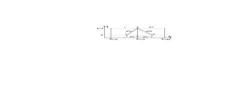
Fig. 3 shows two adjacent cells $i$ and $i+1$. The characteristics in the cell $i$ have index $p_{\,1}$, in the cell $i+1$ – index $p_{\,2}$. One of the characteristics $x^{\,p_{\,1}}\,(t)$ with the eigenvalue $\lambda^{p_{\,1}}>0$ is shown in the cell $i$, another one $x^{\,p_{\,2}}\,(t)$ with the eigenvalue $\lambda^{p_{\,2}}<0$ is shown in the cell $i+1$. According to (24) the amplitude of a wave at point 3, which propagates inside the cell $i$ along the characteristic $x^{\,p_{\,1}}\,(t)$ with the eigenvalue $\lambda^{p_{\,1}}$, is equal to its value at point 1. In the same way the amplitude of a wave at point 3, which propagates inside the cell $i+1$ along the characteristic $x^{\,p_{\,2}}\,(t)$, is equal to its value at point 2.

The state at point 3, which is computed according to (22) by summation with respect to all the eigenvectors, fixed in cell $i$, with $\lambda^{p_{\,1}}>0$ will be on the left side of the interface. Let ${\bf V}^{L}$ denote this value. Similarly, let ${\bf V}^{R}$ denote the state at point 3 on the right side of the interface which is computed by summation with respect to all the eigenvectors fixed in cell $i+1$, with $\lambda^{p_{\,2}}<0$.

The amplitudes of waves $\alpha^{\,p}\,(x^{p},t)$ at the point $x^{p}=x_{i+1/2}-\lambda^{\,p}\,\tau$ in (24), which influence the right boundary of cell $i$ ($\lambda^{\,p}>0$), can be computed by multiplying the expansion (22) by the left eigenvectors, fixed in cell $i$:

$$\alpha^{\,p}\,(x^{p},t)={\bf l}^{\,p}\>{\bf V}(x^{p},t),\quad\lambda^{\,p}>0,$$ (25)

where

$${\bf V}(x^{p})\equiv\frac{1}{x_{i+1/2}-x^{p}}\int^{x_{i+1/2}}_{x^{p}}{\bf V}(x)dx.$$ (26)

We can use arbitrary values for the wave amplitudes for $\lambda^{\,p}<0$ because these waves have no effect on the right boundary of the cell and will be omitted in the sum (22). For convenience let them be

$$\alpha^{\,p}\,(x^{p},t)={\bf l}^{\,p}\>{\bf V}(x_{i},t),\quad\lambda^{\,p}<0.$$ (27)

With the help of $\Theta$-function we can rearrange (25)-(27) as

$$\alpha^{\,p}\,(x^{p},t)=\Theta(\lambda^{\,p})\Bigl{(}{\bf l}^{\,p}\,{\bf V}(x^{p},t)\Bigr{)}+\left(1-\Theta(\lambda^{\,p})\right)\Bigl{(}{\bf l}^{\,p}\,{\bf V}(x_{i},t)\Bigr{)}.$$ (28)

Multiplying (28) by ${\bf r}^{\,p}$ and summing over all $p$ such as $\lambda^{\,p}>0$ according to (22), after some simple manipulations we obtain the boundary value at time $t+\tau$:

$${\bf V}^{L}(x_{i+1/2},t+\tau)={\bf V}(x_{i},t)+\sum_{p\;(\lambda^{\,p}>0)}{\bf r}^{\,p}\left[{\bf l}^{\,p}\Bigl{(}{\bf V}(x^{p},t)-{\bf V}(x_{i},t)\Bigr{)}\right].$$ (29)

If we consider cell $i+1$ and waves with $\lambda^{\,p}<0$ we will obtain a similar expression for the value ${\bf V}^{R}$ on the right side of the interface at time $t+\tau$:

$${\bf V}^{R}(x_{i+1/2},t+\tau)={\bf V}(x_{i+1},t)+\sum_{p\;(\lambda^{\,p}<0)}{\bf r}^{\,p}\left[{\bf l}^{\,p}\Bigl{(}{\bf V}(x^{p},t)-{\bf V}(x_{i+1},t)\Bigr{)}\right].$$ (30)

The left and the right eigenvectors in (29)-(30) are fixed in every cell. To compute them we can use a state from any point $x$ inside the cell - it has been shown by numerical experiments that this choice has no influence on the solution. We suggest using the values of states in the centres of the cells, i.e. ${\bf l}^{\,p}={\bf l}^{\,p}({\bf V}(x_{i},t))$.

Figure 4: Approximation of ${\bf V}(x)$ in the adjacent cells.

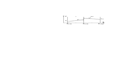
A possible approximation of the component $V(x)$ of the vector-function ${\bf V}(x,t)$ inside grid cells $i$ and $i+1$ at some time step is shown in Fig. 4. The arrows point to the values on the left and the right sides of the interface, note that $V^{L}\neq V^{R}$. The dotted lines are the average values of $V(x)$:

$$V_{i}=\frac{1}{\Delta x}\int\limits_{x_{i-1/2}}^{x_{i+1/2}}V(x)\,d\,x.$$

In order to solve the 3D problem we split the initial set (15) by the space variables and solve the 1D equations separately for the $x$-, $y$- and $z$-directions. However, in this case we have an additional change in the quantities because of the fluxes in the orthogonal directions.

Figure 5: A 2D mesh.

For example, a flux in the $y$-direction will affect the quantities at point 1 between cells $(i,j)$ and $(i+1,j)$ (see Fig. 5). To obtain the correct result, we can solve equation (15) in the $x$-direction considering the terms $B\,\partial_{y}{\bf V}$ and $C\,\partial_{z}{\bf V}$ as sources. Then instead of (23) we arrive at

$$\partial_{\,t}\,\alpha^{\,p}+\lambda^{\,p}\,\partial_{\,x}\,\alpha^{\,p}=-D^{\,p},\quad p=1,\ldots,8,$$ (31)

where $D^{\,p}$ are the components of the vector

$${\bf D}=L_{x}\left(B\>\partial_{\,y}{\bf V}\right)+L_{x}\left(C\>\partial_{\,z}{\bf V}\right).$$ (32)

The components of the partial derivatives in (32) can be calculated as

$$\partial_{\,y}V^{p}=\frac{V^{p}_{i,\,j+1/2,\,k}-V^{p}_{i,\,j-1/2,\,k}}{\Delta y}.$$ (33)

The solution of (31) can be obtained from a Taylor series expansion of $\alpha^{\,p}\,(x,t)$ near the boundary $x=x_{i+1/2}$. It is similar to (24) but has the additional term

$$\alpha^{\,p}\,(x_{i+1/2},t+\tau)=\alpha^{\,p}\,(x_{i+1/2}-\lambda^{\,p}\,\tau,t)-D^{\,p}(t)\,\frac{\tau}{2}.$$ (34)

Then instead of (29)-(30) we arrive at

$${\bf V}^{L}(x_{i+1/2},t+\tau)={\bf V}(x_{i},t)+\sum_{p\;(\lambda^{\,p}>0)}{\bf r}^{\,p}\left[{\bf l}^{\,p}\Bigl{(}{\bf V}(x^{p},t)-{\bf V}(x_{i},t)-D^{\,p}(t)\,\frac{\tau}{2}\Bigr{)}\right],$$ (35)

$${\bf V}^{R}(x_{i+1/2},t+\tau)={\bf V}(x_{i+1},t)+\sum_{p\;(\lambda^{\,p}<0)}{\bf r}^{\,p}\left[{\bf l}^{\,p}\Bigl{(}{\bf V}(x^{p},t)-{\bf V}(x_{i+1},t)-D^{\,p}(t)\,\frac{\tau}{2}\Bigr{)}\right].$$ (36)

In (34)-(36) we have omitted indices $j$ and $k$. The state at point 2 on Fig. 5 is computed in a similar way considering the $x$-derivative as a source.

To obtain states ${\bf V}_{i+1/2}$ in PPML, we solve the Riemann problem for the ${\bf V}^{L}$ and ${\bf V}^{R}$ states on every interface using, e.g., the Roe solver [21] or the HLLD solver [22]:

$${\bf V}_{i+1/2}=R\left({\bf V}^{L},{\bf V}^{R}\right),$$ (37)

where $R$ is the Riemann solver. Note, that in the original PPM, the states ${\bf V}_{i+1/2}$ are obtained through monotonic interpolation [7]. We then apply a monotonicity- and extrema-preserving procedure proposed by Rider et al. [14] to the values of ${\bf V}_{i+1/2}$, as described in Section 6. Finally, we modify the resulting interface states with the standard PPM monotonicity procedure (5)-(6).

So far we have obtained the boundary values of piecewise parabolae at time $t+\tau$ in each grid cell. Now we need to define the fluxes to compute the new central states. Again we can use the Roe solver [21] or the HLLD solver [22] with ${\bf V}^{L}$ and ${\bf V}^{R}$ from (35)-(36) but in this case the numerical scheme will have the first order of temporal accuracy. To design a second order scheme, we must average the amplitudes $\alpha^{\,p}\,(x,t)$ over the zones of influence.

Figure 6: Characteristics inside a grid cell.

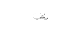
Fig. 6 shows a set of characteristics corresponding to waves with $\lambda^{\,p}>0$. The characteristic $x^{\,1}\,(t)$ has the maximum eigenvalue $\lambda^{\,1}$. Point 1 is the point of intersection between this characteristic and the piecewise parabola at time $t$. Obviously, only the zone between the interface $x=x_{i+1/2}$ and point 1 affects the left boundary state at point 2.

If we consider a wave which propagates along the characteristic with $\lambda^{\,p}>0$ inside cell $i$, its averaged amplitude on the interface $x=x_{i+1/2}$ at time $t+\tau$ can be calculated as

$$\overline{\mathstrut\alpha}^{\,p}_{i+1/2}=\frac{1}{\lambda^{\,p}\,\tau}\int\limits_{x_{i+1/2}-\lambda^{\,p}\,\tau}^{x_{i+1/2}}\alpha^{\,p}\,(x)\,d\,x,\quad\lambda^{\,p}>0.$$ (38)

Multiplying the expansion (22) by the left eigenvectors, fixed in cell $i$, will yield

$$\alpha^{\,p}\,(x)={\bf l}^{\,p}\>{\bf V}(x),\quad\lambda^{\,p}>0.$$ (39)

Inserting (39) into (38) and removing the factor ${\bf l}^{\,p}$ from the integral, we arrive at

$$\overline{\mathstrut\alpha}^{\,p}_{i+1/2}={\bf l}^{\,p}\overline{\vphantom{V^{L}}\,{\bf V}}^{\;L,\,p}_{i+1/2}\,,$$

$$\overline{\vphantom{V^{L}}\,{\bf V}}^{\;L,\,p}_{i+1/2}=\frac{1}{\lambda^{\,p}\,\tau}\int\limits_{x_{i+1/2}-\lambda^{\,p}\,\tau}^{x_{i+1/2}}{\bf V}(x)\,d\,x,\quad\lambda^{\,p}>0.$$ (40)

After that we can arrive at

$$\overline{\vphantom{V^{L}}\,{\bf V}}^{\;L}=\overline{\vphantom{V^{L}}{\bf V}}^{\;L,\,1}_{i+1/2}+\sum_{p\;(\lambda^{\,p}>0)}{\bf r}^{\,p}\left[{\bf l}^{\,p}\Bigl{(}\overline{\vphantom{V^{L}}{\bf V}}^{\;L,\,p}_{i+1/2}-\overline{\vphantom{V^{L}}{\bf V}}^{\;L,\,1}_{i+1/2}-D^{\,p}\,\frac{\tau}{2}\Bigr{)}\right]$$ (41)

which is similar to (35). Here $\overline{\vphantom{V^{L}}{\bf V}}^{\;L,\,1}_{i+1/2}$ is the averaged by formula (40) solution ${\bf V}(x)$ at time $t$ over the zone of influence of the wave in cell $i$, corresponding to the maximum eigenvalue ($\lambda^{\,1}>0$).

For cell $i+1$ and the negative eigenvalues we arrive at

$$\overline{\vphantom{V^{R}}\,{\bf V}}^{\,R}=\overline{\vphantom{V^{L}}{\bf V}}^{\;R,\,1}_{i+1/2}+\sum_{p\;(\lambda^{\,p}<0)}{\bf r}^{\,p}\left[{\bf l}^{\,p}\Bigl{(}\overline{\vphantom{V^{L}}{\bf V}}^{\;R,\,p}_{i+1/2}-\overline{\vphantom{V^{L}}{\bf V}}^{\;R,\,1}_{i+1/2}-D^{\,p}\,\frac{\tau}{2}\Bigr{)}\right],$$ (42)

$$\overline{\vphantom{V^{R}}\,{\bf V}}^{\;R,\,p}_{i+1/2}=\frac{1}{|\lambda^{\,p}|\,\tau}\int\limits_{x_{i+1/2}}^{x_{i+1/2}-\lambda^{\,p}\,\tau}{\bf V}(x)\,d\,x,\quad\lambda^{\,p}<0.$$ (43)

To get the second order of accuracy for time we must compute fluxes on every interface solving the Riemann problem with $\overline{\vphantom{V^{L}}\,{\bf V}}^{\;L}$ and $\overline{\vphantom{V^{R}}\,{\bf V}}^{\,R}$ from (41)-(42). Note that the values of components of the integrals (40) and (43) can be computed as (7) and (8), respectively.

Figure 7: Computation of the component $E_{z}$ at a node.

The time step $\tau$ in (18) is obtained from the Courant condition

$$\tau=\sigma\min_{i,j,k}\left\{\frac{\Delta x}{\left|u_{i,j,k}\right|+c_{f\;i,j,k}^{\,x}},\frac{\Delta y}{\left|v_{i,j,k}\right|+c_{f\;i,j,k}^{\,y}},\frac{\Delta z}{\left|w_{i,j,k}\right|+c_{f\;i,j,k}^{\,z}}\right\},$$ (44)

where $\sigma$ is the Courant number and $c_{f}^{x}$, $c_{f}^{y}$, and $c_{f}^{z}$ are the fast magneto-acoustic velocities along the coordinate directions.

5 Zero divergence constraint for the magnetic field

Our numerical method must provide numerical solutions that satisfy a condition

$${\rm div}\,{\bf B}=0.$$ (45)

There are several approaches to this problem in the literature [18, 23, 24, 25, 17, 26]. In our numerical scheme we used an unsplit Godunov method for ideal MHD with a constrained transport developed in [18] that is based on the Stokes theorem

$$\frac{\partial{\bf\,B}}{\partial\,t}=-\nabla\times{\bf E}.$$ (46)

Calculated from (46) the magnetic field obviously satisfies condition (45). To apply the Stokes theorem in 3D case, we define the magnetic field components on the cell faces and the electric field components on the cell edges. The algorithm exploits the fact that some components of the fluxes ${\bf F}$, ${\bf G}$ and ${\bf H}$ are actually the components of the electric field.

For simplicity let us consider a 2D case. Thus the sixth component of the flux ${\bf F}$ is the $z$-component of the electric field reversed in sign, which correspond to the left and right boundaries of a cell. The fifth component of the flux ${\bf G}$ is the $z$-component of electric field, which correspond to the top and bottom boundaries of a cell. Computing Taylor series for these components near the nodes of the mesh and averaging them, we obtain the components of the electric field at the nodes (Fig. 7).

$$E_{z\;i+1/2,j+1/2}=\frac{1}{4}\left(E^{left}_{z\;i+1/2,j+1/2}+E^{right}_{z\;i+1/2,j+1/2}\right.\\ \left.+E^{top}_{z\;i+1/2,j+1/2}+E^{bottom}_{z\;i+1/2,j+1/2}\right),$$

where for example

$$E^{left}_{z\;i+1/2,j+1/2}=E_{z\;i,j+1/2}+\left.\frac{\partial E_{z}}{\partial x}\right|_{i,j+1/2}\frac{\Delta x}{2},$$

$$\left.\frac{\partial E_{z}}{\partial x}\right|_{i,j+1/2}=\left\{\begin{aligned} \left(\frac{\partial E_{z}}{\partial x}\right)_{i,j},\quad v_{i,j+1/2}>0,\\ \left(\frac{\partial E_{z}}{\partial x}\right)_{i,j+1},\quad v_{i,j+1/2}<0,\\ \frac{1}{2}\left[\left(\frac{\partial E_{z}}{\partial x}\right)_{i,j}+\left(\frac{\partial E_{z}}{\partial x}\right)_{i,j+1}\right],\quad v_{i,j+1/2}=0.\\ \end{aligned}\right.$$

These values of $E_{z\;i+1/2,j+1/2}$ are used in a discrete version of (46):

$$B_{x\;i+1/2,j}^{n+1}=B_{x\;i+1/2,j}^{n}-\frac{\tau}{\Delta y}\left(\vphantom{A^{A^{A}}}E_{z\;i+1/2,j+1/2}-E_{z\;i+1/2,j-1/2}\right),$$

$$B_{y\;i,j+1/2}^{n+1}=B_{y\;i,j+1/2}^{n}+\frac{\tau}{\Delta x}\left(\vphantom{A^{A^{A}}}E_{z\;i+1/2,j+1/2}-E_{z\;i-1/2,j+1/2}\right).$$

Updated components of magnetic field at the center of $(i,j)$-cell are computed by averaging:

$$B_{x\;i,j}^{n+1}=\frac{1}{2}\left(\vphantom{A^{A^{A}}}B_{x\;i-1/2,j}^{n+1}+B_{x\;i+1/2,j}^{n+1}\right),$$

$$B_{y\;i,j}^{n+1}=\frac{1}{2}\left(\vphantom{A^{A^{A}}}B_{y\;i,j-1/2}^{n+1}+B_{y\;i,j+1/2}^{n+1}\right).$$

The magnetic field computed this way will automatically satisfy (45). To make sure that this is indeed the case, ${\rm div}{\bf B}$ should be approximated by the following expression

$$\left({\rm div}\,{\bf B}\right)_{i+1/2,j+1/2}=\frac{1}{2\,\Delta x}\left(\vphantom{A^{A^{A}}}B_{x\;i+1,j}+B_{x\;i+1,j+1}-B_{x\;i,j}-B_{x\;i,j+1}\right)\\ +\frac{1}{2\,\Delta y}\left(\vphantom{A^{A^{A}}}B_{y\;i,j+1}+B_{y\;i+1,j+1}-B_{y\;i,j}-B_{y\;i+1,j}\right).$$

6 Monotonicity constraints

A standard PPM monotonicity preserving procedure (5)-(6) is insufficient for the ideal MHD case. We need to use additional procedures to suppress spurious oscillations.

Procedure 1. To keep a solution monotonic without reducing the order of the scheme and to preserve all the local extrema in MHD simulations we can follow a number of approaches described in the literature [12, 13, 14, 15]. In our method we rely on a Piecewise Parabolic Accurate Monotonicity- and Extrema-Preserving procedure described in [14].

We compute the wave amplitudes $\alpha_{i}^{p}$ for the central states ${\bf V}_{i}$ and $\alpha_{i\pm 1/2}^{p}$ for the interface states ${\bf V}_{i\pm 1/2}$. We then calculate new values for wave amplitudes of the interface states:

$$\alpha_{i\pm 1/2}^{p,\,*}={\rm median}\left(\alpha_{i}^{p},\alpha_{i\pm 1/2}^{p},\alpha_{i\pm 1}^{p}\right)$$

and

$$\alpha_{i\pm 1/2}^{p,\,**}={\rm median}\left(\alpha_{i}^{p},\alpha_{i\pm 1/2}^{p,\,*},3\alpha_{i}^{p}-2\alpha_{i\mp 1/2}^{p,\,*}\right),$$

where the ${\rm median}$ function is defined in a usual way

$${\rm median}\left(a,b,c\right)=a+{\rm minmod}\left(b-a,c-a\right)$$

through the ${\rm minmod}$ function

$${\rm minmod}\left(a,b\right)=\frac{1}{2}\left({\rm sign}(a)+{\rm sign}(b)\right)\min\left(|a|,|b|\right).$$

If $\alpha_{i\pm 1/2}^{p,\,**}=\alpha_{i\pm 1/2}^{p}$ for all $p$, the procedure is completed. Otherwise, we compute a set of fifth-order WENO interface values $\alpha_{i\pm 1/2,*}^{p}$, using Algorithm 2.2.4 from [14], and check for a local extremum. If $\alpha_{i\pm 1/2}^{p,\,**}=\alpha_{i}^{p}$ for all $p$, we apply Algorithm 2.1.2, 4(b), otherwise the region is monotonic but too steep to be approximated with the values obtained from the Riemann solver (37) and we apply Algorithm 2.1.2, 4(c).

Procedure 2. To keep a solution monotonic in a multidimensional case, we employ a method proposed in [16].

Let us consider a 2D case for simplicity. A parabola that approximates a solution along the $x$-axis for every component $V(x)$ of a state ${\bf V}(x,t)$ at some point in time can be defined as

$$V(x)=V_{\,i,j}+\phi(V)\left[s_{\,i,j}\,(x-x_{i})+\frac{\sigma_{\,i,j}}{2}\left((x-x_{i})^{2}-\frac{\Delta x^{2}}{12}\right)\right],$$

where

$$s_{\,i,j}=\frac{V_{i+1/2,j}-V_{i-1/2,j}}{\Delta x},\quad\sigma_{\,i,j}=6\,\frac{V_{i+1/2,j}-2V_{i,j}+V_{i-1/2,j}}{\Delta x^{2}}.$$

As a limiting function $\phi(V)$ we can use that described in [16]:

$$\phi(V)=\min\left(1,\frac{|V_{i,j}-\max(V_{l,m})|}{|V_{i,j}-\max(V_{i-1/2,j},V_{i+1/2,j},V_{i,j-1/2},V_{i,j+1/2})|},\right.\\ \left.\frac{|V_{i,j}-\min(V_{l,m})|}{|V_{i,j}-\min(V_{i-1/2,j},V_{i+1/2,j},V_{i,j-1/2},V_{i,j+1/2})|}\right),$$ (47)

where $l=i-2,i-1,i,i+1,i+2$, $m=j-2,j-1,j,j+1,j+2$ except $(l,m)=(i,j)$. In a 3D case, the limiting function (47) must include all the neighbors of the cell $(i,j)$.

7 A FORTRAN implementation

The algorithm for computing the left and the right boundary values ${\bf V}^{L}$ and ${\bf V}^{R}$ (35)-(36) could be implemented in FORTRAN this way:

integer n, n2

real dt, dx

real VL(8), VC(8), VR(8), Vm(8), V(8), D(8), dVy(8)

real Lambda(8), sumL(8), VLnew(8), VLinterface(8)

real B(8,8), L(8,8), R(8,8)

call Eigenvalues(VC,Lambda) ! compute the eigenvalues at the center of the

! cell $i$ (VC - a state in the center)

if (Lambda(1).gt.0.) then     ! if $\lambda^{1}>0$ then compute a new state VLnew

! on the left side of the interface between the

! cells $i$ and $i+1$

VLnew=0.

xi=1.- Lambda(1)*dt/dx      ! $\xi$ in (1) for $\lambda^{1}$ (see (4))

call Vxi(xi,VL,VC,VR,Vm)   ! formula (1); VL, VR - the left and the right

! boundary values of a parabola, Vm - the result

call MatrixB(VC,B)             ! compute the matrix $B$

call Vectors(VC,L,R)          ! compute the left (L) and right (R) eigenvectors

D=0.

do n=1,8

do n2=1,8

D(n)=D(n)+B(n,n2)*dVy(n2)/dy   ! $\left(B^{\,p}\>\partial_{\,y}V^{p}\right)$ (see (32)-(33))

enddo

enddo

D=D*dt/2.

sumL=0.

do n=1,8

if (Lambda(n).gt.0.) then   ! only these waves affect the interface

xi=1.- Lambda(n)*dt/dx     ! $\xi$ in (1) for $\lambda^{p}$

call Vxi(xi,VL,VC,VR,V)   ! V - the result (a state at the point $\xi$)

do n2=1,8

sumL(n)=sumL(n)+L(n,n2)*(V(n2)-Vm(n2)-D(n2)) ! a part of (35)

enddo

do n2=1,8

VLnew(n2)=VLnew(n2)+R(n2,n)*sumL(n) ! a part of (35)

enddo

end if

enddo

VLnew=Vm+VLnew           ! the result for (35)

else                              ! if the maximum eigenvalue $\lambda^{1}<0$

VLnew= VLinterface     ! we keep the old value on the left side of the interface

end if

A FORTRAN code for computing $\overline{\vphantom{V^{L}}\,{\bf V}}^{\;L}$ and $\overline{\vphantom{V^{R}}\,{\bf V}}^{\,R}$ is similar. We only need to replace the function call call Vxi(xi,...) with one that computes the integral (7) or (8), using

xi=Lambda(1)*dt/dx

or

xi=-Lambda(8)*dt/dx ,

respectively. Lambda(8) is the maximum absolute value of the negative eigenvalue.

To obtain a monotonic solution for a 3D MHD problem, we suggest using the following algorithm:

1. Compute the average interface states $\overline{\vphantom{V^{L}}\,{\bf V}}^{\;L}$ and $\overline{\vphantom{V^{R}}\,{\bf V}}^{\,R}$ from (41)-(42).

2. Solve Riemann problem between $\overline{\vphantom{V^{L}}\,{\bf V}}^{\;L}$ and $\overline{\vphantom{V^{R}}\,{\bf V}}^{\,R}$ to determine the fluxes.

3. Use a conservative difference scheme (18) to compute new central states.

4. Modify the magnetic field at the centers accordingly, see section 5.

5. Compute the interface states ${\bf V}^{L}$ and ${\bf V}^{R}$ from (35)-(36).

6. Solve Riemann problem between ${\bf V}^{L}$ and ${\bf V}^{R}$ to determine the new interface states.

7. Apply procedure 1 in $x$-direction (section 6).

8. Apply procedure 1 in $y$-direction (section 6).

9. Apply procedure 1 in $z$-direction (section 6).

10. Apply procedure 2 (section 6).

11. Apply PPM procedure (5)-(6).

Note that only the interface states are modified by the monotonicity preserving procedures. The solution of the Riemann problem joins the interface values, but the monotonicity procedures split them again into the left and right values.

8 Numerical tests

8.1 Riemann problem with multiple weak discontinuities

This is a 1D problem from [27]. An interval $x\in[0\ldots 1]$ is divided in two by $x=0.5$. The left and the right states at the initial moment are defined as

$$\left(\rho^{\,L},u^{\,L},v^{\,L},w^{\,L},B_{y}^{\,L},B_{z}^{\,L},p^{\,L}\right)=(1.08,1.2,0.01,0.5,3.6,2,0.95),$$

$$\left(\rho^{\,R},u^{\,R},v^{\,R},w^{\,R},B_{y}^{\,R},B_{z}^{\,R},p^{\,R}\right)=(1,0,0,0,4,2,1),$$

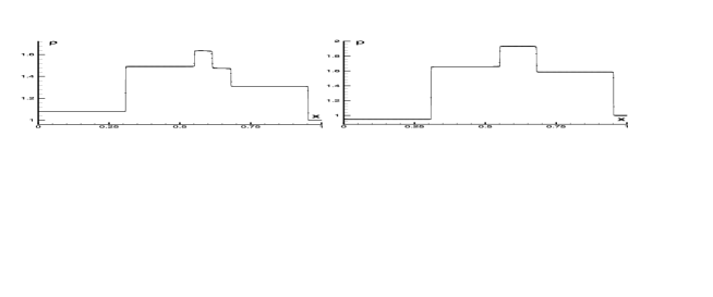
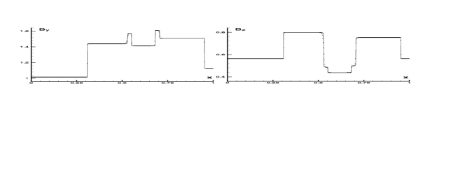
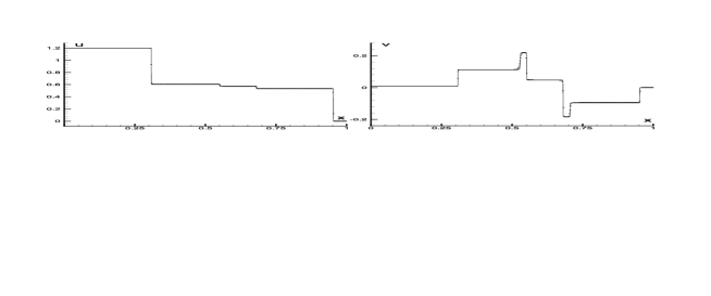
$B_{x}=2$, $\gamma=5/3$, $N=512$. The solution involves two fast shocks with Mach numbers 1.22 and 1.28, two slow shocks with Mach numbers 1.09 and 1.07, two rotational and one contact discontinuities. The solution for the moment $t=0.2$ is presented in Figs. 8-10. The solid line represents the exact solution and points represent the numerical one. PPML produces very sharp fronts resolved with only a few grid points.

Figure 8: Riemann problem with multiple weak discontinuities. Density and pressure distributions.

Figure 9: Same as in Fig. 8 but for $y$- and $z$-components of the magnetic field.

Figure 10: Same as in Fig. 8 but for $x$- and $y$-components of the velocity.

8.2 Numerical dissipation and decay of Alfvén waves

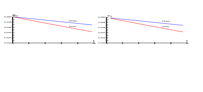
Numerical calculations on a discrete grid always lead to energy loss due to numerical dissipation. In order to estimate the properties of numerical dissipation of the PPML ideal MHD scheme, we used the test problem from [28] and followed a decay of two-dimensional Alfvén wave. We used a standing wave propagating along the grid diagonal with initial conditions

$$\delta v_{x}=v_{amp}\>c_{a}\>\sin(k_{x}x+k_{y}y),$$

$$\delta\rho=\delta p=\delta v_{x}=\delta v_{y}=\delta B_{x}=\delta B_{y}=\delta B_{z}=0$$

in a stationary background flow with $\rho_{0}=1$, $p_{0}=1$, $B_{x}=1$, $B_{y}=B_{z}=0$. This gives the sound speed $c=1.291$ and the Alfvén velocity $c_{a}=0.7071$. The computational domain is a square box with size $L=1$ divided into $64\times 64$ grid cells. The wavenumbers $k_{x}=k_{y}=2\pi/L$, the total wave number $k=\sqrt{k_{x}^{2}+k_{y}^{2}}=\sqrt{2}(2\pi/L)$, the initial peak amplitude $v_{amp}=0.1$, adiabatic exponent $\gamma=5/3$. Computations were carried out with a Courant number $\sigma=0.4$. We used the periodic boundary conditions.

Figure 11 shows the envelope for the maxima of $z$-component of the magnetic field and velocity obtained with PPML and PPM reconstruction procedures as a function of time. While both schemes show very low dissipation, PPML dissipation is even smaller than that of PPM.

Figure 11: Decay of Alfvén waves. The maximum values of $B_{z}$ and $v_{z}$ as a functions of time.

8.3 Travelling circularly polarized Alfvén wave problem

This problem was suggested in [23] as a test for numerical accuracy of smooth flow solutions. The circularly polarized Alfvén wave propagates at an angle of $\alpha=30^{{\rm o}}$ with respect to an axis $x$ in the domain $[0,1/\cos\alpha]\times[0,1/\sin\alpha]$. The initial conditions are

$$\rho=1,\quad v_{\parallel}=0,\quad v_{\perp}=0.1\sin(2\pi\xi),\quad w=0.1\cos(2\pi\xi)$$

$$B_{\parallel}=1,\quad B_{\perp}=0.1\sin(2\pi\xi),\quad B_{z}=0.1\cos(2\pi\xi),\quad p=0.1,$$

where $\xi=x\cos\alpha+y\sin\alpha$. For convenience the parallel and the orthogonal to the direction of Alfvén wave propagation components of the velocity and the magnetic field are used instead the of the components $u$, $v$, $B_{x}$ $B_{y}$. For example $B_{\parallel}=B_{x}\cos\alpha+B_{y}\sin\alpha$, $B_{\perp}=B_{y}\cos\alpha-B_{x}\sin\alpha$. Alfvén wave travels to the point $(x,y)=(0,0)$ with the velocity $B_{\parallel}/\sqrt{\rho}=1$. Note that the wave becomes standing if $v_{\parallel}=1$.

Figure 12: The orthogonal component $B_{\perp}$ in travelling Alfvén wave in computations on meshes with $N=8$, $16$, $32$ and $64$.

Table 1: Travelling Alfvén wave. The average relative errors and the rates of convergence at $t=0.5$.

$N$	$\bar{\delta}_{N}$	$R_{N}$
8	$2.2384\times 10^{-1}$	-
16	$5.7258\times 10^{-2}$	1.967
32	$1.7031\times 10^{-2}$	1.755
64	$5.0365\times 10^{-3}$	1.771

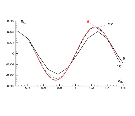
The problem was solved on a set of rectangular $N\times 2N$ meshes with $N=8$, $16$, $32$ and $64$. The averaged relative numerical errors were estimated as

$$\delta_{N}(U)=\frac{\sum\limits_{i=1}^{N}\sum\limits_{j=1}^{2N}|U_{i,j}^{N}-U_{i,j}^{E}|}{\sum\limits_{i=1}^{N}\sum\limits_{j=1}^{2N}|U_{i,j}^{E}|},\quad\mbox{for}\;U=v_{\perp},w,B_{\perp},B_{z},$$ (48)

where the solution on the mesh $N=128$ regarded as the exact one $U_{i,j}^{E}$. The rate of convergence was calculated as follows

$$R_{N}={\rm log}_{2}\left(\delta_{N/2}/\delta_{N}\right),$$ (49)

where $\delta_{N}$ is an averaged value:

$$\delta_{N}=\frac{1}{4}\left(\vphantom{r^{A}}\delta_{N}(v_{\perp})+\delta_{N}(w)+\delta_{N}(B_{\perp})+\delta_{N}(B_{z})\right).$$ (50)

Figure 13: Rotor problem. The contours represent thirty levels of the density in the range from 1.3 to 13.5 and the pressure in the range from 0.12 to 2.1 at $t=0.15$.

Figure 14: Rotor problem. The lines represent thirty levels of absolute value of the magnetic field in the range from 0.32 to 2.288 and the Mach numbers in the range between 0.144 and 4.27 at $t=0.15$.

The calculations were carried out up to $t=5$ with a Courant number $\sigma=0.4$ and $\gamma=5/3$. We applied periodic boundary conditions. Figure 12 demonstrates the convergence of the numerical solution. It shows the orthogonal component $B_{\perp}$ in travelling Alfvén wave for computations on meshes of different size $N$. Table 1 gives average relative numerical errors and rates of convergence obtained for the PPML scheme.

8.4 Rotor problem

The Rotor problem was suggested in [26] and has been widely used to test numerical schemes [e.g., 23, 29, 30]. It turned out to be a hard nut to crack for many codes due to the appearance of negative pressure values [23].

The computational domain in this case is a square $[0,1]\times[0,1]$ with a uniform pressure $p=1$ and magnetic field components $B_{x}=5/\sqrt{4\pi}$, $B_{y}=0$. There is a rotating disk of dense fluid at the center with a radius $r_{0}=0.1$. For $r<r_{0}$ we specify $\rho=10$, $u=-v_{0}(y-0.5)/r_{0}$, $v=v_{0}(x-0.5)/r_{0}$, where $r=\sqrt{(x-0.5)^{2}+(y-0.5)^{2}}$, $v_{0}=2$. For $r>r_{1}=0.115$ the fluid is initially at rest ($u=v=0$) with density $\rho=1$. In the intermediate zone $r_{0}<r<r_{1}$ we use a linear interpolation of the variables: $\rho=1+9f$, $u=-fv_{0}(y-0.5)/r$, $v=fv_{0}(x-0.5)/r$, $f=(r_{1}-r)/(r_{1}-r_{0})$. In this setup, the initial configuration is imbalanced due to centrifugal forces. The rotating fluid will tend to equilibrate, while the magnetic field holds the oblate shape of the rotor.

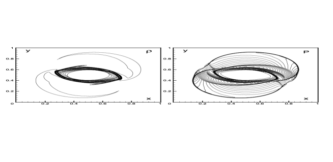
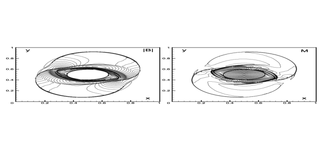
The computations were carried out on a set of $N\times N$ meshes with $N=50$, 100, 200 and 400, with a Courant number $\sigma=0.4$ and $\gamma=1.4$ until $t=0.15$. The boundary conditions are obtained through zero-order interpolation. Figures 13 and 14 show the flow fields for $N=400$.

Table 2: The rotor problem. The average relative errors and the rates of convergence in the numerical codes at $t=0.15$.

N	PPML		Flash3 USM-MEC
	$\bar{\delta}_{N}$	$R_{N}$	$\bar{\delta}_{N}$	$R_{N}$
50	$9.4274\times 10^{-2}$	-	$1.1470\times 10^{-1}$	$-$
100	$4.5204\times 10^{-2}$	1.06	$5.9800\times 10^{-2}$	0.94
200	$1.9262\times 10^{-2}$	1.24	$2.5000\times 10^{-2}$	1.26

We compare numerical solutions obtained with PPML with those presented in [23, 29, 30]. In Table 2 the average relative numerical errors and the rates of convergence are given for PPML and for Flash3 USM-MEC (unsplit staggered mesh algorithm with modified electric field construction introduced in [30]). Both PPML and Flash3 USM-MEC codes use a Roe solver [21] for this test. The relative numerical errors were computed using eq. (48), where for $U_{i,j}^{E}$ we used the highest resolution result ($N=400$). The average error $\bar{\delta}_{N}(U)$ is defined as the average $\delta_{N}(U)$ for all non-zero variables $U$. The rate of convergence is estimated as in (49). PPML results are more accurate and have a comparable rate of (self-)convergence with those from the new Flash3 MHD solver.

Figure 15: Orszag-Tang vortex problem. The contours represent thirty levels of pressure equally spaced in the range from 0.02 to 0.5 at $t=0.5$.

Figure 16: Orszag-Tang vortex problem. The pressure along the lines $y=0.3125$ and $y=0.4277$ at $t=0.5$.

8.5 Orszag-Tang vortex problem

This problem was suggested in [31] and since then has been used in many papers as a standard test problem for numerical codes in 2D MHD. It involves formation and an interaction of multiple shocks and a transition to supersonic turbulence.

In the computational domain $[0,1]\times[0,1]$, we set a uniform density $\rho=25/(36\pi)$ and pressure $p=5/(12\pi)$ with $\gamma=5/3$ (in this case the sound velocity $c=\sqrt{\gamma p/\rho}=1$). The initial velocities and components of the magnetic field are set using harmonic functions: $u=-\sin 2\pi y$, $v=\sin 2\pi x$, $w=0$, $B_{x}=-B_{0}\sin 2\pi y$, $B_{y}=B_{0}\sin 4\pi x$, $B_{z}=0$, where $B_{0}=1/\sqrt{4\pi}$. Despite such smooth initial conditions the fluid motion becomes very complex.

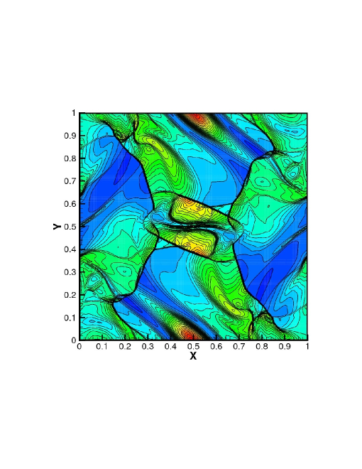
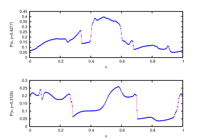
We carried out computations on $N\times N$ meshes with several values of $N$ using periodic boundary conditions and a Courant number $\sigma=0.3$. Figure 15 demonstrates the pressure distribution at time $t=0.5$ for $N=256$. In Fig. 16 the pressure distributions along the lines $y=0.3125$ ($j=83$) and $y=0.4277$ ($j=112$) are shown to illustrate the accuracy and sharpness of the main flow features.

Table 3 contains the average relative numerical errors and the rates of convergence for PPML and Flash3 USM-MEC [30] solvers at $t=0.5$. As an “exact” solution $U_{i,j}^{E}$, we used a solution obtained on the grid with $N=400$. The corresponding PPML results are more accurate and demonstrate better convergence.

Table 3: Orszag-Tang vortex problem. The averaged relative errors and the rates of convergence in the numerical codes at $t=0.5$.

N	PPML		Flash3 USM-MEC
	$\bar{\delta}_{N}$	$R_{N}$	$\bar{\delta}_{N}$	$R_{N}$
50	$8.9095\times 10^{-2}$	-	$1.0160\times 10^{-1}$	$-$
100	$4.4249\times 10^{-2}$	1.013	$5.2200\times 10^{-2}$	0.964
200	$1.8851\times 10^{-2}$	1.235	$1.9900\times 10^{-2}$	1.390

9 A compressible turbulence simulation

Magnetized supersonic turbulence plays an important role in statistical star formation theories [35]. This stimulated development of accurate numerical methods suitable for modeling turbulent molecular clouds. One of the motivations behind the design of PPML has been a need for an MHD scheme with low numerical dissipation comparable or better than that of PPM. In this section we illustrate the performance of PPML on a challenging problem of forced super-Alfvénic turbulence. Some numerical methods that successfully pass the tests discussed above turn unstable on this application. Since adding more dissipation where needed – the usual way to cure for “blow ups” caused by numerical instabilities – would ultimately damage the derived statistics of turbulence [33], the issue of inherent stability of numerical methods is crucial for both supersonic turbulence and star formation simulations.

Figure 17: Supersonic turbulence simulation with PPML on a $512^{3}$ grid. Four snapshots show the density field on a slice $x\equiv 0$ illustrating a transition to fully developed turbulence with $M_{s}\approx M_{A}\approx 10$. The transition includes formation of first strong shocks on the caustics of the initial solenoidal velocity field ($t=0.5t_{d}$, top-left), shock interactions and active development of first shear instabilities ($t=1t_{d}$, top-right), and a gradual transition to a statistical steady state ($t=2t_{d}$ and $4t_{d}$, bottom row). The standard logarithmic black-red-white color ramp shows high-density regions in light-red and rarefactions in black.

For illustrative purposes, we present here a simulation of weakly magnetized supersonic turbulence. In this experiment, turbulence in a periodic domain of linear dimension $L=1$ is driven by a large-scale solenoidal force for 8 flow-crossing times $t_{d}\equiv L/2M_{s}$. At time $t=0$, a uniform gas with density $\rho\equiv 1$ is permeated by a weak uniform magnetic field ${\bf B}_{0}\parallel\boldsymbol{x}$, such that $\beta_{0}\equiv 2p/B_{0}^{2}=20$. We apply an initial large-scale velocity field that corresponds to an rms sonic Mach number $M_{s}\sim 10$ and assume an isothermal equation of state ($c\equiv 1$) to mimic the average physical conditions in the dense parts of molecular clouds ($n=10^{3}$ cm^-3, $T=10$ K).

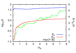
The evolution begins with the formation of strong shocks on “caustics” of the initial velocity field. Shock interactions then cascade the initial kinetic energy of large-scale motion of the gas down to smaller and smaller scales á la Kolmogorov-Richardson, see Fig. 17. The magnetic field gets amplified by a factor of about 50 via the small-scale dynamo action [34]. The large-scale solenoidal force (acceleration) keeps the rms sonic Mach number roughly constant at $M_{s}\approx 10$. The evolution of kinetic and magnetic energies is shown in Fig. 18, left panel. Also shown is $max(\left|\boldsymbol{\nabla\cdot}{\bf B}\right|)$ as a function of time during this simulation. The method keeps the absolute value of the divergence of magnetic field below $10^{-12}$ at all times, even after 70,000 integration time steps (if double precision is used). After about 4 crossing times of evolution, the system completes a transition to a fully developed isotropic state with $M_{s}\approx 10$ and $M_{A}\approx 10$. The right panel of Fig. 18 illustrates spectral characteristics of this saturated state by showing the time-average (over 25 flow snapshots taken between $t=4t_{d}$ and $t=8t_{d}$) power spectra for the density, velocity, and magnetic field strength.

 

Figure 18: Supersonic turbulence simulation with PPML on a $512^{3}$ grid. Time-evolution of kinetic and magnetic energy and maximum absolute value of $\boldsymbol{\nabla\cdot}{\bf B}$ (left panel) and turbulent power spectra for the velocity, density and magnetic field (right panel).

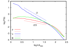
The velocity spectrum has an extended scaling range with a slope of about $-2$, as in the Burgers turbulence, similar to the corresponding scaling in non-magnetized flows at high Mach numbers [32]. This is expected, as turbulence here is only weakly magnetized. The density spectrum slope of about $-0.7$ is again consistent with our previous results for non-magnetized flows obtained with PPM ($-1.0$ at $M_{s}=6$) and with an anticipated trend towards a flat “white noise” spectrum at $M_{s}=\infty$. The magnetic energy spectrum does not show a clear scaling range, as expected at this modest resolution, assuming the effective magnetic Prandtl number of PPML is of order unity. We also looked at more advanced spectral characteristics for compressible flows, such as the power spectrum of $\rho^{1/3}{\bf v}$, and found a slope of $-1.7$. This power spectrum related to the energy transfer rate in wavenumber space is insensitive to the turbulent Mach number and should have a Kolmogorov $-5/3$ slope [32] in both incompressible and highly compressible regimes, although a steeper scaling does occur due to intermittency [36]. This is true for both non-magnetized and weakly magnetized flows.

We have also carried out two additional simulations of the same kind but with higher degrees of magnetization, $\beta_{0}=2$ and 0.2 [37]. While the saturated turbulent state in the $\beta_{0}=2$ variant is still super-Alfvénic with $M_{A}\approx 3$ and the magnetic energy is about 3 times smaller than the kinetic energy, the trans-Alfvénic case, $\beta_{0}=0.2$, reaches an equipartition of kinetic and magnetic energies. In both cases, PPML proved to be perfectly stable at a Courant number $\sigma=0.2$, as in the super-Alfvénic case $\beta_{0}=20$ discussed above.

Our approach to handle the stability issues in MHD turbulence simulations with PPML is as follows: (i) we use locally multidimensional reconstruction that improves the quality of Right and Left interface states and helps to avoid numerous well-known pathologies, such as “carbuncles”, etc. [38]; (ii) we control the quality of these states before moving forward with the flux calculation; (iii) if we find that the states are not satisfactory, we reduce the order of reconstruction to linear or further skip the whole reconstruction step; (iv) we use only nonlinear Riemann solver in all cases lacking the reconstruction step.

Overall, the derived spectral properties of weakly magnetized highly compressible turbulence demonstrate that low dissipation and wide spectral bandwidth of PPML make it an ideal numerical scheme for large-scale simulations of magnetized supersonic turbulence.

10 Conclusions

In this paper we presented PPML, a new numerical method for compressible ideal MHD that is based on the piecewise parabolic approximation. Interface values for the interpolation parabolae in every grid cell are defined with the help of the Riemann invariants which remain constant along the characteristics. The monotonicity of the states on the interfaces between adjacent cells is provided by the monotonicity- and extrema-preserving procedure from [14]. The scheme is fully multidimensional as it includes the terms corresponding to the tangential directions in the amplitude equations. This helps to avoid numerous well-known pathologies, such as “carbuncles”, etc.

The states in the cell centers are defined by the conservative difference scheme (18). To obtain the second-order temporal accuracy we must average the wave amplitudes over the corresponding domains of influence. To define the fluxes we need to solve the Riemann problem between the states at the cell interfaces computed with the averaged amplitudes.

To preserve zero divergence of the magnetic field in three dimensions, we use an unsplit Godunov method based on the constrained transport approach [18]. We use the information about the magnetic field gradients to fulfill the constraint on the magnetic field more accurately.

We tested the performance of PPML on several numerical problems which demonstrated its high accuracy on both smooth and discontinuous solutions. Two-dimensional flow fields generated by PPML are highly resolved without any wiggled contour lines. Our pilot simulations of supersonic magnetized turbulence in three dimensions with PPML show that low dissipation and wide spectral bandwidth of this method make it an ideal candidate for direct turbulence simulations.

References

- [1] M. V. Popov, and S. D. Ustyugov, Piecewise parabolic method on local stencil for gas dynamic simulations, Comput. Mathem. and Mathem. Phys. 47, Issue 12, 1970 (2007).
- [2] M. V. Popov, and S. D. Ustyugov, Piecewise parabolic method on local stencil for ideal magnetohydrodynamics, Comput. Mathem. and Mathem. Phys. 48, Issue 3, 477 (2008).
- [3] P. Colella, P. Woodward, The piecewise parabolic method for gasdynamical simulations, J. Comput. Phys. 54, 174 (1984).
- [4] P. Woodward, P. Colella, The numerical simulation of two-dimensional fluid flow with strong shocks, J. Comput. Phys. 54, 115 (1984).
- [5] W. Dai, P. R. Woodward, Extension of the Piecewise Parabolic Method to multidimensional ideal magnetohydrodynamics, J. Comput. Phys. 115, 485 (1994).
- [6] P. Woodward, The PPM compressible gas dynamics scheme, in “Implicit Large Eddy Simulation: Computing Turbulent Fluid Dynamics”, eds. F. F. Grinstein, L. G. Margolin, and W. J. Rider, Cambridge University Press, p. 130 (2007).
- [7] B. van Leer, Towards the ultimate conservative difference scheme. II. Monotonicity and conservation combined in a second-order scheme, J. Comput. Phys. 14, 361 (1974).
- [8] V. Guinot, High resolution Godunov-type schemes with small stencils, Internat. J. Numer. Methods Fluids 44, 1119 (2004).
- [9] R. Sanders, A third-order accurate variation nonexpansive difference scheme for single nonlinear conservation laws, Mathem. Comput. 51, 535 (1988).
- [10] R. Sanders, A. Weiser, A high order staggered grid method for hyperbolic systems of conservation laws in one space dimension, Comput. Methods Appl. Mech. Eng. 75, 91 (1989).
- [11] R. Sanders, A. Weiser, High resolution staggered mesh approach for nonlinear hyperbolic systems of conservation laws, J. Comput. Phys. 101, 314 (1992).
- [12] A. Suresh, H. T. Huynh, Accurate monotonicity-preserving schemes with Runge-Kutta time stepping, J. Comput. Phys. 136, 83 (1997).
- [13] D. S. Balsara, C.-W. Shu, Monotonicity preserving weighted essentially non-oscillatory schemes with increasingly high order of accuracy, J. Comput. Phys. 160, 405 (2000).
- [14] W. J. Rider, J. A. Greenough, J.R. Kamm, Accurate monotonicity- and extrema-preserving methods through adaptive nonlinear hybridizations, J. Comput. Phys. 225, 1827 (2007).
- [15] P. Colella, M. D. Sekora, A limiter for PPM that preserves accuracy at smooth extrema, J. Comput. Phys. 227, 7069 (2008).
- [16] T. J. Barth, On unstructured grids and solvers, Comput. Fluid Dynamics (Von Kármán Institute for Fluid Dynamics, 1990), Lecture Series 1990-04.
- [17] C. R. Evans, J. F. Hawley, Simulation of magnetohydrodynamic flows: A constrained transport method, Astrophys. J. 332, 659 (1988).
- [18] T. A. Gardiner, J. M. Stone, An unsplit Godunov method for ideal MHD via constrained transport, J. Comput. Phys. 205, 509 (2005).
- [19] A. G. Kritsuk, S. Ustyugov, M. L. Norman, P. Padoan, et al., KITP07 MHD Code Comparison Project, in preparation (2009).
- [20] M. Brio, C. C. Wu, An upwind differencing scheme for the equations of ideal magnetohydrodynamics, J. Comput. Phys. 75, 400 (1988).
- [21] P. L. Roe, Characteristic-based schemes for the Euler equations, Annu. Rev. Fluid Mech. 18, 337 (1986).
- [22] T. Miyoshi, K. Kusano, A multi-state HLL approximate Riemann solver for ideal magnetohydrodynamics, J. Comput. Phys. 208, 315 (2005).
- [23] G. Tóth, The constraint in shock-capturing magnetohydrodynamics codes, J. Comput. Phys. 161, 605 (2000).
- [24] T. I. Gombosi, K. G. Powell, D. L. De Zeeuw, Axisymmetric modeling of cometary mass loading on an adaptively refined grid: MHD results, J. Geophys. Research. 99, 21525 (1994).
- [25] J. U. Brackbill, D. C. Barnes, The effect of nonzero on the numerical solution of the magnetohydrodynamic equations, J. Comput. Phys. 35, 426 (1980).
- [26] D. S. Balsara, D. S. Spicer, A staggered mesh algorithm using high order Godunov fluxes to ensure solenoidal magnetic fields in magnetohydrodynamic simulations, J. Comput. Phys. 149, 270 (1999).
- [27] W. Dai, P. Woodward, An approximate Riemann solver for ideal magnetohydrodynamics, J. Comput. Phys. 111, 354 (1994).
- [28] D. Ryu, T. W. Jones, A. Frank, Numerical magnetohydrodynamics in astrophysics: algorithm and tests for multidimensional flow, Astrophys. J. 452, 785 (1995).
- [29] J. Han, H. Tang, An adaptive moving mesh method for two-dimensional ideal magnetohydrodynamics, J. Comp. Phys. 220, 791 (2007).
- [30] D. Lee, A. E. Deane, An unsplit staggered mesh scheme for multidimensional magnetohydrodynamics, J. Comp. Phys. 228, 952 (2009).
- [31] A. Orszag, C. M. Tang, Small-scale structure of two-dimensional magnetohydrodynamic turbulence, J. Fluid Mech. 90, 129 (1979).
- [32] A. G. Kritsuk, M. L. Norman, P. Padoan, and R. Wagner, The Statistics of Supersonic Isothermal Turbulence, Astrophys. J., 665, 416 (2007).
- [33] H. C. Yee and B. Sjögreen, Development of low dissipative high order filter schemes for multiscale Navier Stokes/MHD systems, J. Comput. Phys., 225, 910 (2007).
- [34] A. A. Schekochihin and S. C. Cowley. Turbulence and Magnetic Fields in Astrophysical Plasmas, p. 85, in Magnetohydrodynamics: Historical Evolution and Trends, (2007).
- [35] C. F. McKee and E. C. Ostriker, Theory of Star Formation, Annual Rev. of Astron. & Astrophys., 45, 565 (2007).
- [36] A. G. Kritsuk, P. Padoan, R. Wagner, and M. L. Norman, Scaling Laws and Intermittency in Highly Compressible Turbulence, AIP Conf. Proc., 932, 393 (2007).
- [37] A. G. Kritsuk, S. D. Ustyugov, M. L. Norman, and P. Padoan, Simulations of Supersonic Turbulence in Molecular Clouds: Evidence for a New Universality, ASP Conf. Series, 406, 15 (2009).
- Quirk [1994] Quirk, J. J., A contribution to the great Riemann solver debate, International Journal for Numerical Methods in Fluids, 18 , 555 (1994).