The chromospherically–active binary CF Tuc revisited

Abstract

This paper presents results derived from analysis of new spectroscopic and photometric observations of the chromospherically active binary system CF Tuc. New high-resolution spectra, taken at the Mt. John University Observatory in 2007, were analyzed using two methods: cross-correlation and Fourier–based disentangling. As a result, new radial velocity curves of both components were obtained. The resulting orbital elements of CF Tuc are: $a_{1}{\sin}i$=$0.0254\pm 0.0001$ AU, $a_{2}{\sin}i$=$0.0228\pm 0.0001$ AU, $M_{1}{\sin}i$=$0.902\pm 0.005$ $M_{\odot}$, and $M_{2}{\sin}i$=$1.008\pm 0.006$ $M_{\odot}$. The cooler component of the system shows H$\alpha$ and CaII H & K emissions. Using simultaneous spectroscopic and photometric observations, an anti-correlation between the H$\alpha$ emission and the $BV$ light curve maculation effects was found. This behaviour indicates a close spatial association between photospheric and chromospheric active regions. Our spectroscopic data and recent $BV$ light curves were solved simultaneously using the Wilson-Devinney code. A dark spot on the surface of the cooler component was assumed to explain large asymmetries observed in the light curves. The following absolute parameters of the components were determined: $M_{1}$=$1.11\pm 0.01$ $M_{\odot}$, $M_{2}$=$1.23\pm 0.01$ $M_{\odot}$, $R_{1}$=$1.63\pm 0.02$ $R_{\odot}$, $R_{2}$=$3.60\pm 0.02$ $R_{\odot}$, $L_{1}$=$3.32\pm 0.51$ $L_{\odot}$ and $L_{2}$=$3.91\pm 0.84$ $L_{\odot}$. The primary component has an age of about 5 Gyr and is approaching its Main Sequence terminal age. The distance to CF Tuc was calculated to be $89\pm 6$ pc from the dynamic parallax, neglecting interstellar absorption, in agreement with the Hipparcos value. The orbital period of the system was studied using the $O-C$ analysis. The $O-C$ diagram could be interpreted in terms of either two abrupt changes or a quasi-sinusoidal form superimposed on a downward parabola. These variations are discussed by reference to the combined effect of mass transfer and mass loss, the Applegate mechanism and also a light-time effect due to the existence of a third body in the system.

1 Introduction

Recently, the study of chromospherically active binaries (hereafter CAB) has become more popular (e.g. Eker et al. (2008) for a third version of the catalogue of CABs; Zhang and Gu (2008) for SZ Psc; Frasca et al. (2008) for $\lambda$ And and II Peg; Strassmeier et al. (2008) for HD 6286; Fekel et al. (1985) and later series of papers). CAB stars are usually either detached or semi-detached systems and their components include late spectral types of F, G or K, with luminosity classes V or IV. They show large asymmetries in their light curves, that are usually explained in terms of cool/dark spot(s) models. The chromospheric activity is associated with CaII H and K or/and H$\alpha$ emission lines, ultraviolet excess, soft X-rays and radio emission. There is a wealth of associated phenomena - including starspots, plages, flares, non-radiatively heated outer atmospheres, activity cycles, and deceleration of rotation rates.

The study of such active binary stars provides understanding of the origin, evolution, and effects of magnetic fields in cool stars. In this context, we have chosen CF Tuc as the target of the present work. A review of this binary is presented below, new spectroscopic observations and their reductions are described in Section 2. The procedure used to obtain radial velocities and the orbital solution are outlined in Section 3, while rotation velocities of the components are examined in Section 4. Magnetic activity indicators, H$\alpha$ and CaII H & K emission lines, are examined in Section 5, while simultaneous solutions of the $BV$ light and radial velocity curves are given in Section 6. The orbital period analysis is reviewed in Section 6, and a discussion of the new results is given in the last section.

CF Tuc (HD 5303 = HIP 4157, $V$ = 7.60 mag) is a well known southern hemisphere CAB. In the third edition of the CAB catalogue, recently published by Eker et al. (2008), the following physical properties are given: (i) It is a RS CVn-type SB2 system with the spectral types G0V/IV+K4IV/V (Cutispoto and Leto (1997)). (ii) Photometric light curves have remarkable asymmetries, especially visible well out of eclipses. The magnitudes of these asymmetries are variable with time (e.g. Budding and Zeilik (1995); Anders et al. (1999)). (iii) Radial velocities of the components were obtained, and then spectroscopic orbital elements and absolute parameters of the components were derived: $M_{1}$=1.06 $M_{\odot}$, $M_{2}$=1.21 $M_{\odot}$, $R_{1}$=1.67 $R_{\odot}$, $R_{2}$=3.32 $R_{\odot}$, $T_{1}$=5980 K and $T_{2}$=4210 K (Collier et al. (1981); Coates et al. (1983)). (iv) The orbital period is 2.797672 days, however it is changing (Thompson et al. (1991); Anders et al. (1999); Innis et al. (2003), Innis et al. (2007a)). (v) Orbital inclination is close to 70^∘, therefore eclipses are partial (e.g. Budding and Zeilik (1995); Anders et al. (1999)). (vi) The projected rotational velocities of the components are around 25 – 30 km/s for the primary, 52 - 75 km/s for the secondary (e.g. Coates et al. (2000)). (vii) The spectra of the system give relatively high Li abundance (Randich et al. (1993)). (viii) The system shows strong CaII H and K emission (e.g. Hearnshaw and Oliver (1977)). The H$\alpha$ line appears as nearly totally filled-in absorption (Collier et al. (1982)). (ix) The system is also a known radio and X-ray source (Budding et al. (2002); Pravdo et al. (1996)). Some large flare events were reported (e.g. Kürster and Schmitt (1996)). Other references can be found in the CAB catalogue.

Particular aims of the present study are: (i) to investigate the orbital period changes of CF Tuc with updated data, and (ii) to derive more accurate absolute parameters of the system using our new, high resolution spectroscopic data.

2 Spectroscopic observations

The spectroscopic observations of CF Tuc were made at Mt John University Observatory (hereafter MJUO) in New Zealand in the summer season of 2007. A 1m McLennan telescope and HERCULES (High Efficiency and Resolution Canterbury University Large Échelle Spectrograph) spectrograph were used. The spectrograph has 100 échelle orders, which cover wavelength range between 380 nm and 900 nm, and is located in a vacuum tank on stable ground in a thermally isolated room and attached to the telescope by fibre cables. There are two different resolving powers: R=41000 and R=70000. In the observations the former was used as being better adjusted to the mean seeing value ($\theta$ $\sim$ ${3.5^{\prime\prime}}$) at MJUO given by Hearnshaw et al. (2002).

Table 1: Journal of spectroscopic observations of CF Tuc. Signal-to-noise (S/N) ratio refers to the continuum near 5800 Å.

No	Frame	HJD	S/N	Exp.Time
		(+2450000)		(s)
1	w4350022	54349.98652	60	1509
2	w4350030	54350.03238	74	1223
3	w4350053	54350.23328	78	1322
4	w4351012	54350.89945	85	1144
5	w4351014	54350.91536	80	1021
6	w4352010	54351.90655	50	1500
7	w4352019	54351.96099	78	1500
8	w4352022	54351.98189	85	1200
9	w4353002	54352.86852	85	1500
10	w4354017	54353.93546	80	1300
11	w4354019	54353.95324	85	1300
12	w4354037	54354.10935	95	1300
13	w4354039	54354.12710	88	1300
14	w4356003	54355.85715	55	1600
15	w4356005	54355.87984	60	1700
16	w4356018	54355.99775	70	1500
17	w4356028	54356.07125	80	1500
18	w4356030	54356.09149	80	1500
19	w4363011	54362.85380	98	1600
20	w4363027	54362.93923	80	1900
21	w4363029	54362.96309	85	1750
22	w4377014	54376.89666	94	2100
23	w4377022	54376.96563	78	2200
24	w4378016	54377.94931	82	2100

24 spectra were obtained over 10 nights between September and October 2007. The journal of observations is shown in Table 1. The exposure time was chosen between 1100 and 1800 seconds, depending on the weather conditions. During the observations, comparison spectra of a thorium-argon arc lamp were taken before and after each stellar image. A set of white lamp images was also taken as flat field images. Two IAU radial velocity standard stars (HD 36079 and HD 693) were observed. The bright, non-active and slowly rotating standard star HD 36079 (G5II, $V_{r}$=-13.6 km/s) was chosen for the RV measurements of the components of CF Tuc. Hercules Reduction Software Package (HRSP, ver. 3: Skuljan and Wright 2007) was used for reductions of all observations. This procedure takes into account other sources of apparent motion (such as the Earth’s rotations and orbital revolution), wavelength calibration, removal of spurious pixels (such as those struck by cosmic rays), correction for the inherent pixel-to-pixel response variation (flat-fielding), continuum normalization, etc., and produces a target spectrum (wavelength versus flux) as the result.

3 Radial velocities and the orbital solution

Measurements of radial velocities were done by two methods: The cross-correlation technique (CCT) and the Fourier disentangling technique (KOREL). CCT was used as the first step to estimate the orbital parameters, as KOREL may not produce a unique solution in some complex cases. In this study, the real orbit improvement comes from usage of KOREL and the number of spectral orders is not so relevant to accuracy. In general, if all the spectral orders were of the same quality, the precision of a measurement would increase with the square root of the number of orders. If the best spectral orders are chosen, others will produce systematic errors, and improvement will not be scaled as the square root of the number of orders. The main issue is the role of noise and better line resolution and identification in the selected orders. In the case of CF Tuc, since CF Tuc is rather faint for the used observational instruments and its components are close to G0 V/IV + K4 V/IV, the observed spectra of the system include too many blended metallic absorption lines. It is very difficult to identify real/true lines and to resolve them into two components. All spectral regions were examined, and, as a result, four spectral orders were selected, for which the lines of both components could be clearly detected, and therefore suitable for disentangling. The information about these four spectral orders is given in Table 2.

Table 2: Spectral orders and stellar lines used in RVs measurements of CF Tuc.

Order No	Wavelength	Dominant
	Interval (Å)	Spectral Lines
85	6640-6740	SiII (6660.52 Å), SiII (6665.0 Å)
		FeI (6677.989 Å), SiII (6717.04 Å)
88	6430-6440	FeI (6430.844 Å), CaI (6439.075 Å), CaI (6449.81 Å)
		CaII (6456.87 Å), CaI (6462.57Å)
97	5820-5900	NaI D2 (5892 Å), NaI D1 (5898Å)
110	5151-5188	MgI (5174.13 Å), FeI (5168.897Å), FeII (5169.03 Å)
		FeII (5171.595 Å), MgI (5172.6843 Å), MgI (5174.13 Å)

For the CCT, the FXCOR task in the radial velocity package of IRAF (Tonry and Davis (1979); Popper and Jeong (1994)) was used. FXCOR calculates the velocity Doppler shift between two spectra (of the variable and comparison stars) by fitting the correlation with a user-selected function. In the present study, the Gaussian function was adopted as the best-fitting one. The spectra of HD 36079 were used as a template for deriving RVs of the components. In order to obtain orbital parameters from the radial velocity data derived from the CCT, the ELEMDR77 program, developed by T. Pribulla (2008, private communication), was used.

For the Fourier disentangling technique, the KOREL code (developed by Hadrava (1995), Hadrava (1997)) was used. In the first step with this procedure, KOREL requires input parameters within realistic bounds. The initial values of parameters were taken from the solution of RV curves obtained with the CCT method. Four spectral orders, given in Table 2, were analyzed simultaneously. After several iterations, the KOREL code gave a value close to 0 for the eccentricity $e$ within its uncertainties. For this reason, we assumed a circular orbit for the system. Additionally, during the fitting, the orbital period $P_{orb}$ of the system was fixed to be 2.7975004 days (see Section 5). The velocity amplitudes $K_{1}$ and $K_{2}$ of the components and the conjunction time $T_{0}$ were the adjusted parameters. The best fitting orbital elements are given in Table 3, and the best fits to the composite spectra and disentangled spectra are shown in Fig. 1 for the echelle order 88 as a sample.

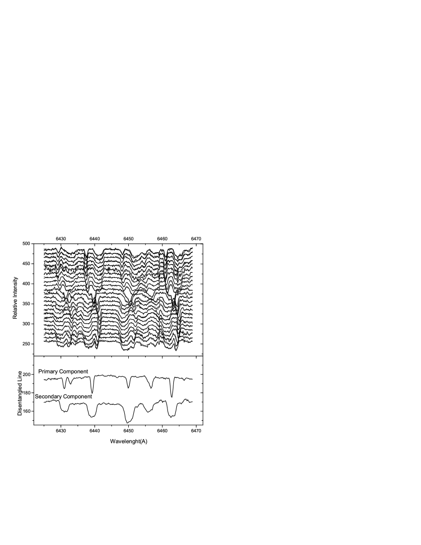
Figure 1: KOREL solution of echelle order 88 as a sample. Upper panel shows the KOREL fits while the lower panel displays the disentangled spectra of each component.

Table 3: Spectroscopic orbital parameters of CF Tuc

Parameter	Value
$P_{orb}$ (days)	2.7975004 (fixed)
$T_{o}$ (HJD)	54327.0583${\pm}$0.0012
$V_{\gamma}$(km/s)	9.58${\pm}$0.14
$q$	1.117${\pm}$0.009
$K_{1}$(km/s)	98.92${\pm}$0.24
$K_{2}$(km/s)	88.55${\pm}$0.24
$a_{1}{\sin}i$(AU)	0.0254${\pm}$0.0001
$a_{2}{\sin}i$(AU)	0.0228${\pm}$0.0001
$M_{1}{\sin}i$(${M_{\odot}}$)	0.902${\pm}$0.005
$M_{2}{\sin}i$(${M_{\odot}}$)	1.008${\pm}$0.006

Table 4: RV measurements, with O–C values from theoretical fit, of components of CF Tuc.

Time	Phase	$RV_{1}$	$O-C_{1}$	$RV_{2}$	$O-C_{2}$
HJD	$\phi$	(km s-1)	(km s-1)	(km s-1)	(km s-1)
2454377.9493	0.192	-82.4	1.0	91.8	-0.5
2454349.9865	0.196	-84.6	-0.4	92.3	-0.8
2454350.0324	0.212	-87.2	-0.2	96.2	0.8
2454352.8686	0.226	-87.9	0.7	96.8	0.0
2454350.2333	0.284	-87.7	-0.7	95.5	0.1
2454355.8572	0.295	-85.3	0.0	94.4	0.6
2454355.8798	0.303	-84.4	-0.7	92.6	0.1
2454355.9978	0.345	-72.5	-0.7	87.0	4.7
2454356.0713	0.371	-62.1	-0.6	73.7	0.3
2454356.0915	0.378	-58.9	-0.5	70.8	0.1
2454350.8994	0.522	24.9	0.5	-	-
2454350.9154	0.528	26.7	-1.3	-	-
2454353.9355	0.608	71.1	-1.7	-45.4	0.9
2454353.9532	0.614	75.7	0.1	-48.2	0.6
2454354.1093	0.670	95.8	-1.3	-67.5	0.6
2454354.1271	0.676	96.0	-2.8	-71.8	-2.2
2454362.8538	0.796	104.3	-0.1	-75.1	0.3
2454376.8967	0.815	100.2	0.0	-70.4	1.4
2454362.9392	0.826	97.3	0.0	-68.8	0.3
2454362.9631	0.835	94.8	0.3	-66.6	0.1
2454376.9656	0.840	93.0	0.2	-65.0	0.2
2454351.9065	0.882	76.3	0.4	-50.0	-0.1
2454351.961	0.902	66.9	0.9	-41.7	-0.5
2454351.9819	0.909	63.1	0.7	-38.2	-0.4

The KOREL code can not derive the systemic velocity of the binary star, however, KOREL retains the systemic velocity in the disentangled spectra of the components. Therefore, the systemic velocity $V_{\gamma}$ was adopted by averaging systemic velocities obtained from the CCT method and the ELEMDR77 program. The adopted systemic velocity was added to the RVs measured by KOREL to yield the final RVs of the components, which are given in Table 4. In this table, phase values of observed time of RVs in the second column were calculated using the linear ephemeris given in Eq. 1. $O$-$C$ values in the fourth and sixth columns represent the residuals between observed and theoretical RVs obtained from simultaneous solution of the $BV$ light and RV curves, described in Section 5.

4 Rotational velocities

The program PROF (Budding and Zeilik (1995)), which follows an ILOT type curve-fitting procedure, was used to determine rotational velocities. PROF convolves Gaussian and rotational broadenings, as discussed by Budding and Zeilik (1995), and computes the line profile as a function, basically, of the following parameters: the continuum intensity $I_{c}$, the relative depth $I_{d}$ at mean wavelength $\lambda_{m}$, the rotational broadening parameter $r$, Gaussian broadening parameter $s$ of a given line, and the limb darkening coefficient $u$. A similar procedure was followed by Olah et al. (1992), Olah et al. (1998) and Budding et al. (2009).

We considered the Na D2 line profiles for CF Tuc in the Hercules spectral order 97 and fitted the selected line profiles at various orbital phases using PROF. Typical results of the profile fitting at phases of 0.371 and 0.826 are shown in Fig. 2 and given in Table 5.

Figure 2: Results of profile fitting to Na D2 5892 lines at phase 0.371 (upper panel) and phase 0.826 (lower panel).

Table 5: Profile fitting parameters at two different orbital phases for the Na D2 5892 feature.

	phase 0.371		phase 0.826
Parameter	Primary	Secondary	Primary	Secondary
$I_{c}$	1.024$\pm$0.015	0.990$\pm$0.010	0.927$\pm$0.012	1.031$\pm$0.008
$I_{d}$	0.216$\pm$0.018	0.188$\pm$0.010	0.192$\pm$0.019	0.175$\pm$0.008
$\lambda_{m}$(Å)	5888.740$\pm$0.043	5891.452$\pm$0.094	5891.852$\pm$0.043	5888.641$\pm$0.102
$r$(Å)	0.498$\pm$0.053	1.142$\pm$0.108	0.528$\pm$0.055	1.216$\pm$0.088
$s$(Å)	0.469$\pm$0.107	0.745$\pm$0.074	0.300$\pm$0.060	1.053$\pm$0.055
$r$(km/s)	25$\pm 3$	58$\pm 6$	27$\pm 3$	62$\pm 5$
$s$(km/s)	24$\pm$6	38$\pm$4	15$\pm$3	54$\pm$3
$\Delta l$	0.01	0.01	0.01	0.01
$\chi^{2}/\nu$	1.034	1.040	1.024	1.048

According to the value of $r$ (the rotational broadening parameter) in Table 5, the projected rotational velocities of the primary and secondary components are 26$\pm 3$ and 60$\pm 5$ kms^-1, respectively. Using absolute parameters of components from Table 8 and $v_{rot}$sin$i$=2$\pi R$sin$i$/$P_{rot}$ (assuming synchronous rotation, $P_{rot}$=$P_{orb}$, and $i_{rot}$=$i_{orb}$), theoretical rotational velocities were be found as 28$\pm 1$ and 62$\pm 2$ kms^-1 for the primary and secondary components, respectively. Therefore, we found that within the error limits, synchronous rotation for both components can be reliably accepted.

The Gaussian broadening parameter $s$ (presented in Table 5) ranges from 24 to 15 km/s for the primary component and from 38 to 54 km/s for the secondary component at phases of 0.371 and 0.826, respectively. This parameter generally relates thermal broadening and other broadening factors (micro and/or macro turbulence, etc.) rather then rotational broadening. If the temperature of 4300 K is taken, where the Na D2 lines are formed in a subgiant atmosphere, thermal velocities are found to be $\sim$2 km/s. Therefore, for this value, the thermal broadening is not significant, and the broadening parameter must include some other motions, possibly related to turbulence effects or magnetic activity. Since our spectroscopic observations and Innis’s CCD $BV$ observations were made almost simultaneously, we can compare these spectroscopic results with the spot model derived from the $BV$ light curve analyses. For instance, when the maculation is close at phase 0.821, the $s$ parameter is greatest and falls to about 38 km/s half a cycle later (at phase 0.371). Therefore, we can deduce that the larger value of $s$ of the secondary component could be associated with the relatively stronger effects of surface activity of this star.

5 Magnetic activity indicators

The H$\alpha$ and CaII H & K emission lines are very important indicators of magnetic activity - in other words, chromospheric activity. Generally, the more active stars show these emission lines always above the continuum (e.g. UX Ari, II Peg, AR Psc, V711 Tau and XX Tri). Except for being sensitive to the chromospheric activity, these emission lines are also a good diagnostic of inter-components matter in the form of gas streams, transient or classical accretion disks and rings in mass-transferring binaries i.e. the Algol type, in which the cooler star fills its Roche lobe and transfers mass to the hot companion (e.g. Richards and Albright (1999)).

The H$\alpha$ and CaII H & K observed line profiles of CF Tuc are shown in Figs. 3, 4 and 5. In these spectra, the H$\alpha$ profiles show absorption and emission features, while the CaII H & K are in emission at all orbital phases. All absorption and emission features were red and blue-shifted depending on the orbital phases. Since the cooler component of the system is an active star, it is assumed that these emission features are related to this component. To confirm this, we calculated the RV values of the H$\alpha$ and CaII K emission features and plotted them in Fig. 6 with RVs of both components of the binary system. We took into account only the K line (3933.66 Å) here, because of likely contamination from H$\epsilon$ centered only 1.5 Å away from the H line (3968.47 Å). As it can be seen in Fig. 6, although not strictly sinusoidal, the RVs of the H$\alpha$ emission feature follows the orbital motion of the cooler component but with a larger amplitude of about 200 kms^-1. This rather larger amplitude indicates that the H$\alpha$ emission feature could originate in a gas cloud in the form of a chromospheric prominence from the cooler component. The RVs of the CaII K emission line closely follows that of the cooler component (see Fig. 6), indicating its origin to be in the chromospheric layers of that star.

Figure 3: Observed H$\alpha$ line profiles for CF Tuc in 2007 at first half (left panel) and second half (right panel) of the orbital period. The vertical lines represent the laboratory wavelength ($\lambda_{0}$=6562.82 Å) of the H$\alpha$ line.

Figure 4: Sample of observed CaII H & K spectra for CF Tuc at different orbital phases.

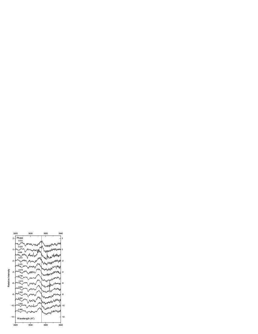
Figure 5: Observed CaII K line profiles for CF Tuc in 2007 at first half (left panel) and second half (right panel) of the orbital period. The vertical lines represent the laboratory wavelength ($\lambda_{0}$=3933.66 Å) of the CaII K line.

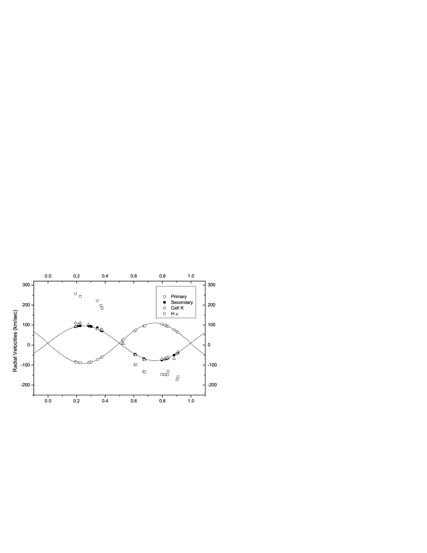
Figure 6: Variations of RVs of emission features observed in H$\alpha$ and CaII K. The continuous lines are the RV solutions for the primary (hotter) and secondary (cooler) components, according to parameters given in Table 6.

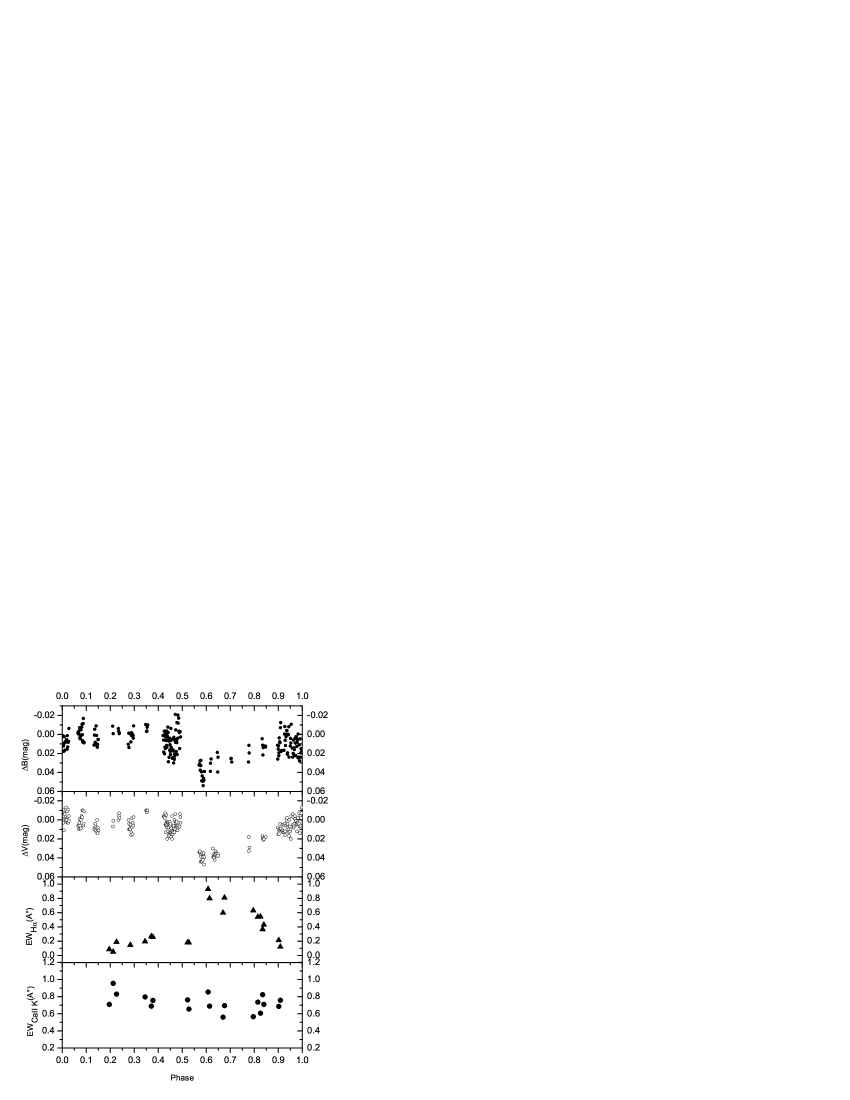
Figure 7: Maculation effects in $BV$ magnitudes (upper two panels), and observed $EW$s of H$\alpha$ and CaII K emission features (lower two panels) as a function of the orbital phase for CF Tuc.

If we assume that the H$\alpha$ emitting region is at rest in the rotating reference frame of the system and that it lies between the barycentre of the system and the cooler component, we can estimate its location following Marino et al. (2001), who modelled inter-components matter using H$\alpha$ lines for HR 7428. The HR 7428 star is an RS CVn-type binary, composed of a bright K giant and an A-type Main Sequence dwarf. It is a well detached system like our target star, CF Tuc. In this model, the projected distance of the emitting region can be found from $a_{er}$=$a_{c}$($K_{er}$/$K_{c}$), where $a_{c}$ is the semi-major axis of the cooler star orbit, and $K_{c}$ and $K_{er}$ are the semi-amplitudes of the RV variations for the cooler star and emitting region, respectively. Since our orbital solution gives $K_{c}$=89 kms^-1 and $a_{c}$=3.6$\times$10⁶ km, we find $a_{er}$=8.2$\times$10⁷ km - in other words, the H$\alpha$ emitting region should be located at a distance of about 2 $R_{c}$ from the surface of the cooler component. We estimate almost the same value for the location of the emitting region using $v_{er,rot}$sin$i$=2$\pi a_{er}$ sin$i$/$P_{rot}$ (with the assumption of synchronous rotation).

The simultaneous photometric and spectroscopic observations of CF Tuc offer the possibility of studying the photospheric (spots) and chromospheric (plages and/or prominences) active regions of the cooler component. With this aim, we measured the equivalent widths ($EW$s) of emission features observed in the H$\alpha$ and CaII K spectra by means of multiple Gaussian fits, and plotted them versus orbital phase in Fig. 7. In Section 6, we present a large cool photospheric spot on the cooler component to explain observed $BV$ light curve asymmetries. To concentrate on effects due to the spot only, we subtracted the eclipse and proximity effects from the observed data using the unspotted (immaculate) light curve parameters given in Table 6 and plotted these points (which show the maculation/distortion wave) versus the orbital phase in the upper panels of Fig. 7.

The maximum $EW_{H\alpha}$ value of about 1 Å is reached at phases 0.6 – 0.7, where the spot effect is dominant ($BV$ distortion of lights minima); the minimum value of $EW_{H\alpha}\cong$0.2 Å is observed between phases 0.0 and 0.5, where the spot could not be seen in the light curves. The CaII K equivalent width does not show any clear orbital modulation (rotational modulation under the synchronous rotation). However, there is a possible anti-correlation between $BV$ light curve asymmetries and H$\alpha$ emission, which is apparent with an almost similar shape of the curves. This behaviour denotes a close spatial association of photospheric and chromospheric active regions. Such anti-correlations between photospheric and chromospheric diagnostics are found in some active stars and have been examined by many authors (e.g. Frasca et al. (2000), Frasca et al. (2005); Biazzo et al. (2006)).

6 Simultaneous Solution of the $BV$ Light and Radial Velocity Curves

We analyzed the $BV$ light curves from Innis, J. L. (2008, private communication), Hipparcos light curve (ESA 1997) and radial velocity curves from this study using the Wilson-Devinney code (WD), version 1996 (Wilson and Devinney (1971)). The $BV$ light curves from Innis and our new radial velocity curves were solved simultaneously. Innis et al. observed CF Tuc in $BV$ filters at Brightwater Observatory in the summer season of 2007. They used a short-focus, 70mm telescope and a cooled SBIG ST7E CCD camera, which gives a field of view of near 0.8 arcdegree$\times$0.55 arcdegree. A detailed description of the observatory and techniques is given in the paper by Innis et al. (2007b). They observed HD 5210 and HD 4644 as comparison and check stars, respectively. We calculated external uncertainties for all comparison minus check magnitudes and found them to be 31 and 13 mmag in $B$ and $V$ filters, respectively. For this, we used the standard deviation of the differential light variations of the comparison relative to the check star collected during the same night. A similar procedure was followed by Erdem et al. (2009) and also Strassmeier et al. (1999) to examine the quality of long-term multicolour photometric data of several active stars. The observational data were not transformed into the standard $BV$ system. It is worth noting that our spectroscopic observations and their photometric observations were made almost simultaneously. In order to calculate the phases of the CCD $BV$ light observations of CF Tuc, the light elements of the system were derived by using the photoelectric primary minima times with $E>$2000 cycles (see Fig. 9b) as;

$$HJD~{}(Min~{}I)=2452452.7326(68)+2^{\rm d}.7975004(9)\times E.$$ (1)

with the weighted least squares method. In the light curves which were formed using these phases, the primary minimum coincides with the phase 0.0 (see upper panel of Fig. 8).

In the WD method, some parameters could be fixed according to theoretical models. In the light curve modelling, the temperature of the primary component was fixed at 6100 K, following Anders et al.(1999) and Budding and McLaughlin (1987). The root square limb darkening law was adopted, and the darkening coefficients were taken from Diaz-Cordoves et al. (1995) and Claret et al. (1995) The bolometric gravity-darkening coefficients of the components were set to 0.32 for convective envelopes, following Lucy (1967); also, the bolometric albedos were fixed to 0.5 for convective envelopes, following Rucinski (1969). According to analysis of the rotational velocities (see Section 4), the components rotate synchronously. Therefore, the rotation parameters were assumed as F_h=F_c=1. From the spectroscopic orbital solution described in Section 3, the circular orbit ($e$=0) was adopted.

Table 6: Final solutions of light and radial velocity curves of CAB star CF Tuc

Parameter	$BV+2RV$	Hp
$a(R_{\odot})$	11.08$\pm$0.02	–
$Phase$ $shift$	-0.0017$\pm$0.0002	-0.0003$\pm$0.0006
$V_{\gamma}$ (km/s)	9.6$\pm$0.4	–
$i$ (deg)	69.91$\pm$0.09	69.91
$T_{1}$ (K)	6100	6100
$T_{2}$ (K)	4286$\pm$19	4286
${\Omega}_{1}$	7.907$\pm$0.086	7.907
${\Omega}_{2}$	4.452$\pm$0.011	4.452
$q_{corr}=m_{2}/m_{1}$	1.115$\pm$0.003	1.115
$l_{1}/l_{12}~{}(B)$	0.616$\pm$0.008	–
$l_{1}/l_{12}~{}(V)$	0.557$\pm$0.008	0.567$\pm$0.001
$r_{1}(mean)$	0.148$\pm$0.001	0.148
$r_{2}(mean)$	0.325$\pm$0.001	0.325
Spot parameters
Spot1 co-latitude (deg)	155$\pm$5	121$\pm$5
Spot1 longitude (deg)	303$\pm$4	329$\pm$3
Spot1 radius (deg)	47$\pm$2	31$\pm$4
Spot1 Tspot/Tstar	0.746$\pm$0.038	0.731$\pm$0.026
Spot2 co-latitude (deg)	–	24$\pm$3
Spot2 longitude (deg)	–	206$\pm$3
Spot2 radius (deg)	–	38$\pm$2
Spot2 Tspot/Tstar	–	0.785$\pm$0.028
$\Sigma W(O-C)^{2}$	0.03177	0.01192

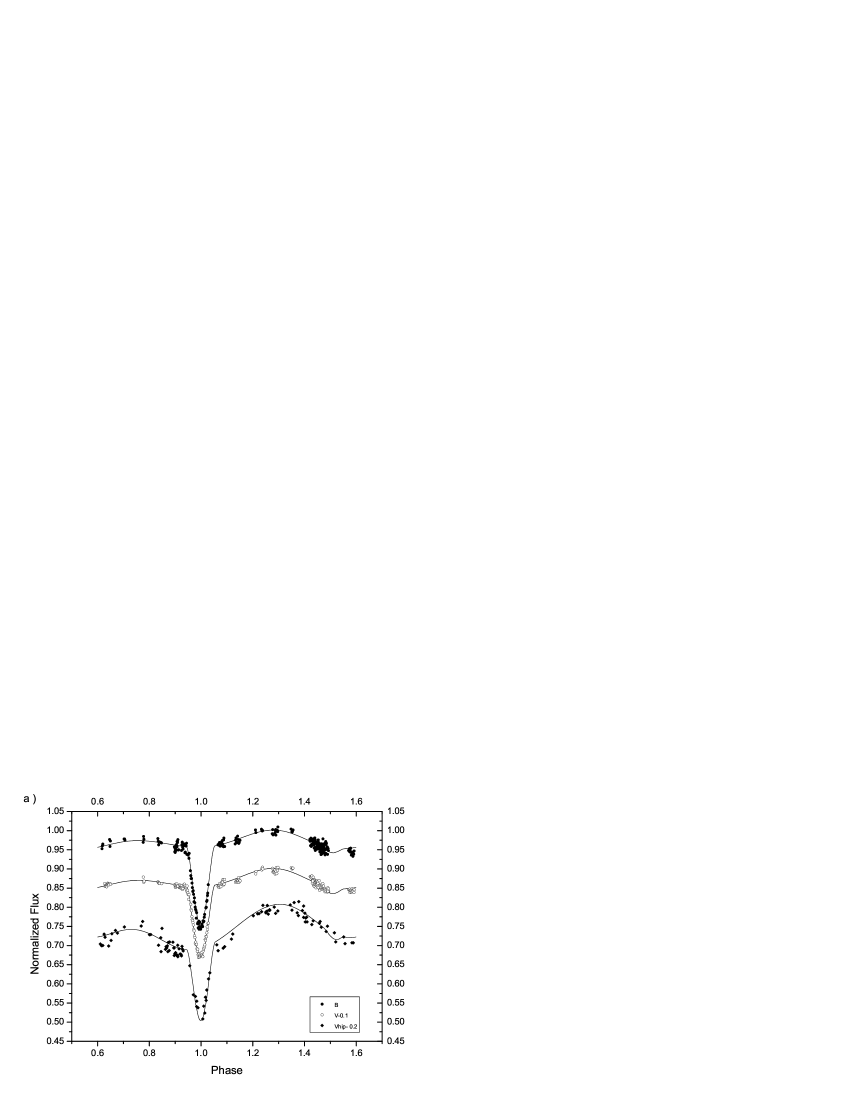
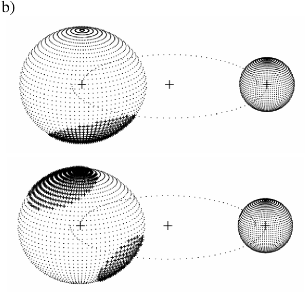
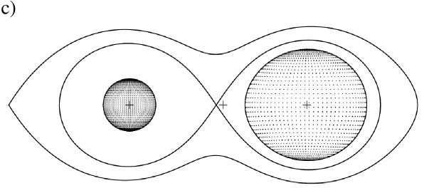
Figure 8: $a)$ Best theoretical fits to the $BV$ and Hipparcos light curves, $b)$ one spot and two spots on the 3D model of the cooler component for the $BV$ and Hipparcos light curves, respectively, and $c)$ Roche geometry of the system.

The adjusted parameters in our computations are: the semi-major axis of orbit ($a$), phase shift, systemic velocity of the binary ($V_{\gamma}$), orbital inclination ($i$), surface temperature of the secondary component ($T_{2}$), non-dimensional surface potentials of both components (${\Omega}_{1}$ and ${\Omega}_{2}$), and the fractional monochromatic luminosity of the primary component (l₁/(l₁+l₂)). The initial values of $q$, $A$ and $V_{\gamma}$ were taken from the radial velocity solution (see Section 3). Due to the probability of the existence of a third body, resulting from the orbital period analysis of the system (see Section 7), a third light contribution ($l_{3}$) was also considered as a free parameter. However, we soon found its contribution to be negligible. The binary CF Tuc, as mentioned above, is a typical RS CVn type eclipsing binary and its light curves show distortion wave like other systems in this group. In the $BV$ light curves, the distortion wave appears to be an asymmetry between the light levels of the maxima (see Fig. 8a). Therefore, we had to consider a cool spot on the secondary and allowed the spot parameters to be adjusted.

In order to get good starting parameters for the WD code, mean points were calculated from all individual observations. This provided standard deviations for $B$ and $V$ filters; the highest values were 15 mmag (the clump near phase 0.9) in $B$, and 11 mmag (near phase 0.1) in $V$. These mean points (69 in $B$, 64 in $V$) were used with a Monte Carlo search to find a fit to the $BV$ light curves with a mass ratio fixed at the value derived spectroscopically (see Table 3). The resulting parameters were next set as starting values for simultaneous solution of the $BV$ light and RV curves. Simultaneous $BV$ light and RV curves solution was done for all individual points, assigning the same weight and different errors for the $B$ and $V$ filters as resulted from the calculation of mean points. Errors for the RV curves were assigned the same as their quality was comparable. The NOISE control parameter was set to 1.

Simultaneous convergent solutions of the BV light and RV curves were obtained by iterations, until the corrections of the parameters became smaller than their corresponding errors. The results of the final solution are given in Table 6. The comparison between observed and computed light curves is shown in Fig. 8a, while that of RV curves is presented in Fig. 6. The three-dimensional model demonstrating the presence of a large dark spot on the surface of the cooler component and the Roche geometry of the system (making use of the Binary Maker program, ver.3.0, Bradstreet and Steelman (2002)) are also shown in Fig. 8b,c.

We made additional attempts to check the stability of our solution. This was done by assigning larger errors for the photometric light curves (especially for the $B$ light curve). Additionally, only RV curves (adjusting only the parameters relevant to the orbit) were solved using the WD code. It was found that the simultaneous solution of $BV$ and RV curves resulted in the mass ratio q=1.115$\pm$0.003, while only the RV solution gave q=1.113$\pm$0.004. Also, the solutions with assigned larger errors for $B$ data gave (within uncertainties) a similar value of the mass ratio.

The Hipparcos light curve of CF Tuc is available from the Hipparcos web page and contains 121 points with an average observational error of 11 mmag. Before starting analysis, Hipparcos observations of the system were transformed to Johnson $V$ magnitudes using $Hp-V$ = 0.22$\times$($B-V$) calibration given by Rucinski and Duerbeck (1997).

The following ephemeris was used to phase the Hipparcos photometric data:

$$HJD~{}(Min~{}I)=2448502.560+2^{\rm d}.79765\times E.$$ (2)

The data was weighted by using the equation $w_{i}=1/\sigma_{i}^{2}$, where $\sigma_{i}$ is the individual standard error of the data given in the Hipparcos catalogue. About ten photometric points were discarded due to their relatively large errors. We used the mean maxima levels at phase 0.25 for the flux normalization of both the Hipparcos and 2007 $BV$ filters data.

During the iterations, only spot parameters, phase shift, and luminosity of the primary component were treated as free parameters; others were adopted from the simultaneous solution of $BV$ and radial velocity curves. As can be seen in Fig. 8a, the Hipparcos light curve shows two large asymmetries, one at about phase 0.70 and another at the primary minimum. Therefore, the possibility of two dark spots on the secondary component was considered. The final results are given in Table 6 and displayed in Fig. 8a,b.

7 Orbital period analysis

In order to investigate the orbital period variation of the system, we gathered 33 minima times available from the lists compiled by Kreiner, J. M. (2008, private communication) and Anders et al. (1999) and we added one minimum time, which was calculated from the 2007 $BV$ light curves observed by Innis et al. (2008, private communication). As a first step, $O-C$ values were calculated using the following light elements, given by Anders et al. (1999):

$$HJD~{}(Min~{}I)=2444219.270+2^{\rm d}.797715\times E.$$ (3)

The $O-C$ values versus $E$ values (and years) were found and the results are shown in the upper panel of Fig. 9a,b. Thompson et al. (1991) first noted that the orbital period of the system changes in the form of an upward parabola and tried to explain this variation in terms of a mass transfer or a mass loss from the system. Anders et al. (1999) showed that the orbital period change has a cyclic character and discussed the $O-C$ diagram, the spot-wave amplitude and the mean light change of the system as being due to the Applegate mechanism. Innis et al. (2003) and Innis et al. (2007a) reported that the orbital period of the system did not show any change between 1995 and 2006. Therefore, we could say that the real nature of the period variation shows up as the data increases by time.

In the present $O-C$ analysis, due to a large scatter, one spectroscopic time of minimum obtained by Hearnshaw and Oliver (1977) was discarded and altogether 33 photometric data were used. The standard errors of observed minima times, as given by authors, are shown as error bars in Fig. 9a,b. The weights were assigned according to these errors. As the standard errors are given in 4, 3 and 2 decimal places, we used 10, 7 and 5 for weights, respectively. The observed long–term period decrease of CF Tuc from these $O-C$ diagrams could thus be explained as follows:

(i) Abrupt period changes: The $O-C$ diagram in Fig. 9a was considered in terms of abrupt period changes. Period jumps might have occurred two times within an interval of about 30 years. Considering that the period has remained constant between these two jumps, we calculated following three linear ephemerides. The first ephemeris valid for $E$ $\leq$ 776 is:

$$HJD~{}(Min~{}I)=2444219.2615(52)+2^{\rm d}.797692(12)\times E,$$ (4)

for 885 $\leq$ $E$ $\leq$ 1835 we have:

$$HJD~{}(Min~{}I)=2444219.2126(51)+2^{\rm d}.797749(4)\times E,$$ (5)

and finally for $E$ $\geq$ 2192 we have:

$$HJD~{}(Min~{}I)=2444219.7446(153)+2^{\rm d}.797482(5)\times E.$$ (6)

The first abrupt period change $\Delta P/P$=($-2.04\pm 0.31$)$\times 10^{-5}$ occurred at HJD 2446527$\pm$70; while the second one $\Delta P/P$=($+9.51\pm 0.06$)$\times 10^{-5}$ occurred at HJD 2449745$\pm$100. The time interval between these two possible abrupt period changes was taken as 3218$\pm$105 days (or approximately 9 years). Such sudden period jumps could be caused by anisotropic mass ejections from one (or both) component(s) (e.g. Huang (1963)). Indeed, the RVs of H$\alpha$ emission support such a high velocity ejecting gas from the active component (see Section 5), like a prominence in the solar atmosphere. However, as seen in Fig. 9a, the sudden period changes seem to have occurred in the pattern of one period increase and a subsequent decrease. This might be an indication of sinusoidal variations rather than abrupt period changes due to sudden mass ejections.

(ii) Continuous period change and the light-time travel effect: A reasonable fit to the $O-C$ data is obtained by using a sinusoidal ephemeris with a quadratic term, as

$$C=T_{0}+P\times E+Q\times E^{2}+A_{s}sin[\frac{2\pi}{P_{s}}(E-T_{s})],$$ (7)

where $A_{s}$ is the semi-amplitude, $P_{s}$ the period and $T_{s}$ the time of minimum. However, to show the parabolic $O-C$ change clearly, we recalculated $O-C$ values by using the following light elements;

$$HJD~{}(Min~{}I)=2448922.2310+2^{\rm d}.797630\times E.$$ (8)

These new $O-C_{2}$ values were then plotted against the epoch number and observation years in the second panel of Fig. 9b. This panel shows a simple downward parabola, where the axis of symmetry is parallel to the $O-C$–axis with the vertex at epoch number $E$=0. It should be noted that the best model fitting both $O-C_{1}$ and $O-C_{2}$ values yields the same values within uncertainties for both quadratic and sinusoidal terms. Finally, parameters of the best theoretical curve fitting the $O-C$ data are given in Table 7, and the best theoretical fit with the observational data is plotted in Fig. 9b.

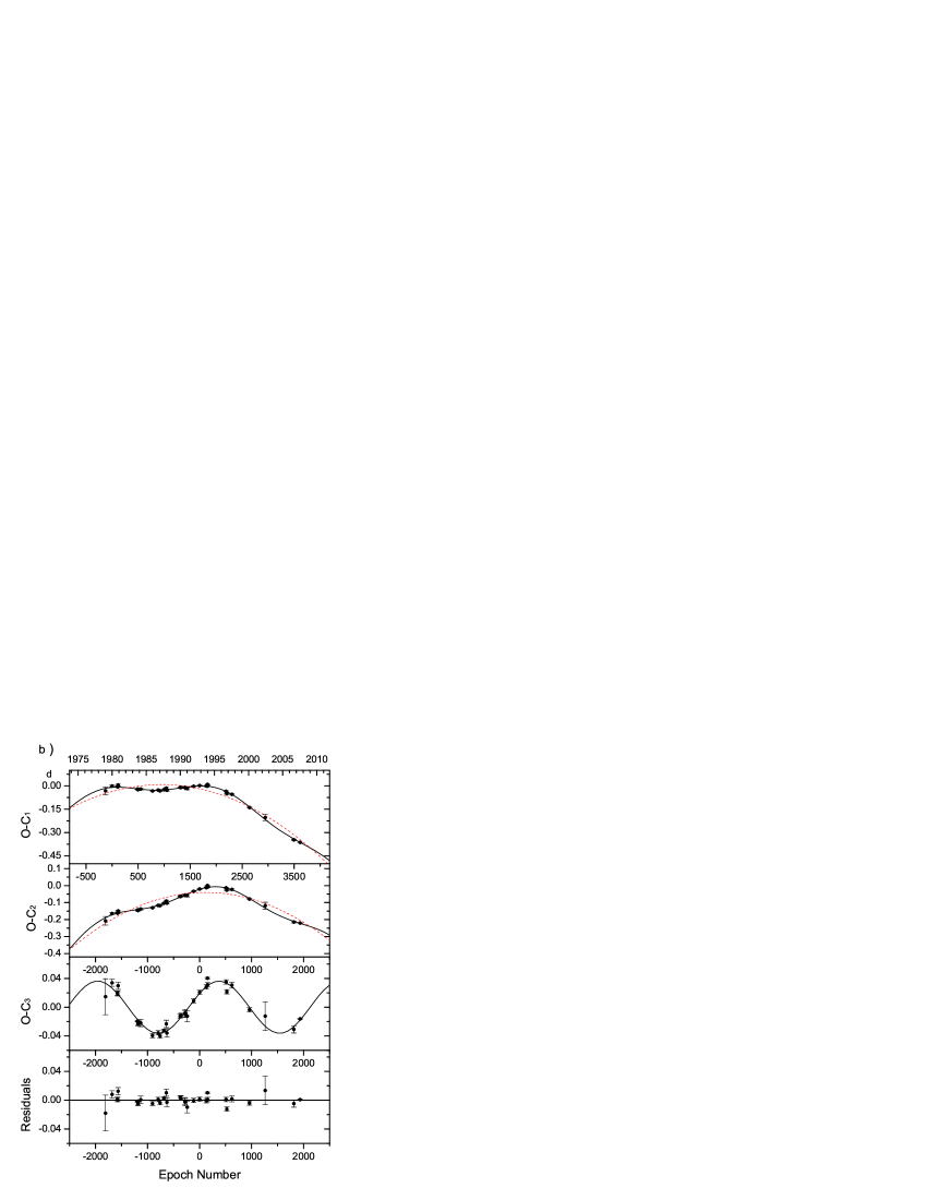
Figure 9: $(a)$ $O-C$ diagram of CF Tuc constructed with Eq. (3). It shows that the period variation of the system could be interpreted in terms of two abrupt period changes. The residuals were calculated separately with the three linear ephemerides given Eqs. (4,5,6). $(b)$ Sinusoidal representation (solid line) is superimposed on the parabolic form (dashed line) of the $O-C$ variation of CF Tuc, and the residuals from the best fit curve. The $O-C_{1}$ values in the top panel were calculated by using the linear ephemeris of Anders et al. (1999), while those of $O-C_{2}$ in the second panel were computed by Eq. (8) to show a symmetric parabola at the vertex with $E$=0. These panels show the same parabola + sinusoidal variation. $(c)$ Systemic velocity variations in CF Tuc. The individual points show observed systemic velocities; the continuous curve is the radial velocity curve corresponding to the light-time orbit in Table 7. $(d)$ A relative astrometric orbit of CF Tuc about a barycentre with a third body. The points represent Hipparcos astrometric data, while the solid curve corresponds to the astrometric solution given in Table 7.

Table 7: Parameters for the CF Tuc sinusoidal O-C solution + astrometry.

Parameter	Value
Sinusoidal O-C solution
$T_{0}$ (HJD)	2448922.2102${\pm}$ 0.0021
$P$ (d)	2.797641${\pm}$ 0.0000015
$Q$ (d)	$-4.9\times 10^{-8}{\pm}2.1\times 10^{-9}$
$A_{s}$ (d)	0.0363${\pm}$ 0.0018
$P_{s}$ (yr)	17.87${\pm}$ 0.57
$T_{s}$ (HJD)	2430387${\pm}$ 599
$\Sigma W(O-C)^{2}$	0.00848
Astrometry solution
$P_{12}$ (yr)	17.87
$T_{12}$ (HJD)	2443441
$a_{12}$ (mas)	72.04
$e_{12}$	0
$\omega_{12}$ (deg)	90
$i_{12}$ (deg)	83 ${\pm}$ 7
$\Omega_{12}$ (deg)	144 ${\pm}$ 19
$\Delta\alpha cos\delta$ (mas)	37.4${\pm}$0.2
$\Delta\delta$ (mas)	56.4${\pm}$0.2
$\Delta\mu_{\alpha}cos\delta$ (mas/yr)	-2.9${\pm}$0.3
$\Delta\mu_{\delta}$ (mas/yr)	0.7${\pm}$0.3
$\Delta\Pi$ (mas)	-0.7${\pm}$0.3
$\chi^{2}/\nu$	1.01

According to the quadratic term given in Table 7, the orbital period of CF Tuc is continuously decreasing at a very rapid rate of $1.11\pm 0.05$ seconds per year. Here, CF Tuc appears to have the highest rate of period decrease among the RS CVn systems. We considered the combined effect of the mass loss and the mass transfer to study this observed period decrease of the system and used the following equation, given by Erdem et al. (2007a) and Erdem et al. (2007b):

$$\frac{\Delta P}{P}=3\left(\frac{r_{A}}{a}\right)^{2}\frac{\delta M}{M}+3\frac{(M_{l}-M_{g})}{M_{l}M_{g}}\Delta M,$$ (9)

where the mass $\Delta M$ is transferred from the mass–losing component to the gainer, the $\delta M$ is the amount of mass lost from the system after co–rotating with the system up to the distance $r_{A}$ (i.e. Alfvén radius), and $\Delta P/P$ is the period change. Since CF Tuc is a detached system, in which the primary and secondary components are filling $\sim 52\%$ and $\sim 89\%$ of their lobes (see Section 6), a direct mass transfer between components is not expected. However, the secondary component is a magnetically active and larger star, which is not far from filling its Roche lobe, and then there could be weak coronal flow from this component to the primary component through the inner Lagrangian point. Therefore, the active component might have a strong stellar wind, which drives the mass loss and mass transfer in the system. The RVs of $H\alpha$ emission support such a strong stellar wind, which reaches twice the larger distance than the radius of the active, subgiant component (see Section 5). If we assume that the transferred mass due to the wind from the secondary to the primary component and the co-rotating distance are $10^{-11}$ $M_{\sun}$/yr and $10R_{2}$, respectively, then Eq. (9) gives the mass loss rate of $\delta M$ = $3.38\times 10^{-7}$ $M_{\sun}$/yr for the observed period change of $\Delta P/P$ = $-4.57\times 10^{-6}$ yr^-1. It is worth mentioning that this mass loss rate is 10 times higher than the maximum value of the range between 10^-11 and $10^{-8}$ $M_{\sun}$/yr given by Hilditch (2001) for the mass losses due to winds from red-giant stars.

There are two plausible causes of the sinusoidal $O-C$ variation: a light-time effect due to a third body in the system and a period modulation due to the magnetic activity cycle of one of the components. We shall investigate these suggested hypotheses in turn.

According to Table 7, CF Tuc would have a circular orbit around the center of the mass of a three-body system and its period would be $17.87\pm 0.57$ yr. The projected distance of the center of mass of the eclipsing binary to that of the three-body system would be $6.29\pm 0.31$ AU. These values lead to a large mass function of $f(M_{3})$ = $0.78\pm 0.07$ $M_{\sun}$ for the hypothetical third body. The mass of such a third body would then range from $9.63\pm 0.29$ $M_{\sun}$ for $i_{12}$=30^∘ to $2.71\pm 0.13$ $M_{\sun}$ for $i_{12}$=90^∘. Here the sum of masses was taken as $M_{1}$ + $M_{2}$=2.34 $M_{\sun}$ (see Section 8). If the third body were co–planar with the eclipsing pair, its mass and the radius $r_{3}$ of its orbit around the center of mass of the three-body system would be about $2.99\pm 0.13$ $M_{\sun}$ and 4.93 AU, respectively. This value of $r_{3}$ is smaller than the radius of the orbit of Jupiter, however, it shows that the third body would revolve far beyond the outer Lagrangian points of CF Tuc, and its orbit should be stable. If we consider the distance of CF Tuc as 89 pc (see Table 8), the minimum projected angular separation between the third star and the eclipsing pair could be estimated as $\sim 71$ mas.

The semi-amplitude of the radial velocity of the center of mass of the eclipsing pair, relative to that of the three-body system, is derived to be 10.5 km/s, which is a convenient value for modern spectroscopic observations to resolve reliably. The theoretical variation of the systemic velocity of CF Tuc, caused by the orbital motion around the common barycentre, is illustrated in Fig. 9c. There are three values of the systemic velocity observed at different epochs: 12.1$\pm$4.7 km/s (Collier et al. (1981)), 0.5$\pm$1.6 km/s (Balona (1987)), and 9.6$\pm$1 km/s (present study). Except for the first data point, the observed systemic velocities follow the long-term variation corresponding to the light-time orbit in Table 7 and are almost the same (within their standard erros) as the theoretical values. The velocity measurement by Collier et al. (1981) is affected by a relatively large error, which could be caused by the scatter of RV data points and the two year time span of their observations.

The astrometric method was also used to check the third body hypothesis. A similar procedure was applied by Ribas et al. (2002) for R CMa, by Bakış et al. (2005) and Bakış et al. (2006) for XY Leo and $\delta$ Lib, by Budding et al. (2009) for U Oph and also Zasche and Wolf (2007) for VW Cep, $\zeta$ Phe and HT Vir. We used the Hipparcos Intermediate Astrometric Data (ESA (1997)) for this. Hipparcos observed CF Tuc between January 1990 and January 1993. There are 76 one-dimensional astrometric measurements corresponding to 40 different epochs in the Hipparcos Intermediate Astrometric Data, which were obtained by the two Hipparcos data reduction consortia: FAST and NDAC. These data are available from the Hipparcos web page. In fact, the astrometric method gives support to the third body hypothesis on orbital period analyses of eclipsing binaries in two ways: one is to plot an orbit of the eclipsing binary about the barycentre of a three-body system and the other is to determine its orbital inclination ($i_{12}$). We followed the procedure applied by Budding et al. (2009) for our target. In this procedure, an orbital model, which is derived from the orbital motion of the eclipsing binary around the barycentre of a three-body system, is convolved with the astrometric motion (parallax and proper motion). This model has 12 independent parameters: $a_{12}$, $e_{12}$, $\omega_{12}$, $i_{12}$, $P_{12}$, $T_{12}$ (periastron passage time), $\Omega_{12}$ (seven for the orbital parameters), and $\alpha$, $\delta$, $\mu_{\alpha}$, $\mu_{\delta}$, $\Pi$ (five for the astrometric components; equatorial coordinates + proper motion + parallax). Since the Hipparcos astrometric data cover only 1/6 part of the orbital period of the hypothetical three-body system, we could take only two parameters from the orbital parameters, $i_{12}$ and $\Omega_{12}$, together with five adjustable astrometric parameters. The final results are given in Table 7 and Fig. 9d. The orbital inclination of CF Tuc in the triple system is, $i_{12}$, about 83^∘ and gives the mass of a third body as about 2.74 $M_{\sun}$. Unfortunately, since the time span of the Hipparcos observations is much shorter than the orbital period of the three-body system and is not the periastron passage of CF Tuc in the three-body orbit, the data, as shown in Fig. 9d, cover only a small part of the orbit.

An alternative way of explaining the O-C behavior would be Applegate’s mechanism (Applegate (1992)). According to this, the cyclic magnetic activity could produce orbital period modulations, which are observed in some eclipsing binaries, especially in RS CVn type systems. Magnetic activity can change the quadrupole moment of a component as the star goes through its activity cycle. The cyclic exchange of angular momentum between the inner and outer parts of the star can change both the shape and radial differential rotation of the star. The torque required for such transfer of angular momentum could be provided by a subsurface magnetic field of several kG. Any change in the rotational regime of a component of an eclipsing binary due to magnetic activity could be reflected in the orbit, as a consequence of the spin-orbit coupling. Here, we shall use Applegate’s formalization to examine the sinusoidal part of the orbital period variation of CF Tuc and assume that the secondary star could be responsible for the observed orbital period modulation. The $O-C$ diagram of CF Tuc, given in Fig. 9b, shows a modulation with a semi-amplitude of 0.0363 days and a modulation period of 17.87 years. This gives $\Delta P/P$=3.49$\times$10^-5. The change in the orbital period is $\Delta P$=8.45 s. The angular momentum transfer would be $\Delta J$=6.84$\times 10^{48}$ gcm²s^-1. If the mass of the shell is $M_{s}$=0.1$M$, the moment of inertia of the shell is $I_{s}$=1.03$\times 10^{55}$ gcm², and the variable part of the differential rotation is $\Delta\Omega/\Omega$=0.026. The energy budget and RMS luminosity variation are $\Delta E$=9.08$\times 10^{42}$ ergs and $\Delta L_{RMS}$=13.23 $L_{\sun}$. This model gives a mean subsurface field of 12.1 kG. The RMS luminosity variation predicted by this model is larger than the total luminosity of the active star. Therefore, a model with $M_{s}$=0.1$M$ and $\Omega_{dr}$=$\Delta\Omega$ cannot explain the orbital period change observed in CF Tuc. Applegate (1992) has also calculated a similar result for RS CVn itself. However, he could obtain a reasonable result for RS CVn using the following two approaches: one is that the active component has solid body rotation, in which $\Omega_{dr}$=0. The other is energy dissipation in the inner part of the star due to differential rotation and some storage of energy in the convection zone. This energy could be omitted from the luminosity variation. These two modifications lower the luminosity variation by a factor of 4 but we are still left with a large value of $\Delta L_{RMS}$=3.31 $L_{\sun}$=0.85 $L$. Therefore, we conclude that the Applegate mechanism is not sufficient to explain the observed period changes.

8 Results and discussion

The new 24 high-resolution échelle spectra of CF Tuc were analysed and precise spectroscopic orbital elements were obtained by means of two techniques; cross-correlation and spectral disentangling. The KOREL program was applied to four spectral orders, which contain about 15 lines, and then reliable radial velocities of both components of the system were obtained. In the literature, there are two spectroscopic studies on CF Tuc: Collier et al. (1981) and Balona (1987). Authors of the former obtained 31 spectra of the system between 1976 and 1978 and used H_δ absorption and CaII H and K emission lines to derive radial velocities of both components. However, their data have a large standard error of 14 km/s, and their spectroscopic orbital elements were less accurate than these presented in this work. Balona (1987) gave radial velocity measurements of only the hotter component and its orbital solution.

Using the observed spectral lines with high precision (i.e. Na D2 line), we found the components of CF Tuc to be in synchronous rotation. In fact, the derived rotational velocity of this secondary star is puzzling, a point which was examined by Coates et al. (2000). They noted that there is a discrepancy between measurements of the rotational velocity of the secondary published in the literature (Budding and McLaughlin (1987); Anders et al. (1999); Donati et al. (1997)). The rotational velocity of the primary (hotter component) ranges from 25 to 30 km/s, which is similar within uncertainties, while that of the secondary component is 52 to 70 km/s, which corresponds to a rather large range of values in the secondary star radius, from 3 $R_{\odot}$ to 4.3 $R_{\odot}$. Coates et al. (2000) used the measurements of Donati et al. (1997) and emphasized that the projected rotational velocity of the secondary should be $\sim 70$ km/s from the derived absolute parameters of the system if the components rotated synchronously.

Our radial velocity and the 2007 $BV$ light curves from Innis, were simultaneously solved using Wilson-Devinney code. The 2007 $BV$ light curves show large asymmetry in the two different maxima similar to those observed in RS CVn type eclipsing binary stars. CF Tuc is a bright system ($V\cong 7.6$ mag), and has been frequently observed photometrically. In the last three decades about 30 light curves of the system were obtained; almost all of them exhibit large asymmetries. The secondary component is apparently magnetically active, as Collier et al. (1981) observed the indicator of magnetic activity, CaII H & K emission lines, from this component. Our H$\alpha$ and CaII H & K observations also show that the secondary component is a chromospherically (or magnetically) active star. Therefore, these light asymmetries were considered as maculation effects and interpreted using spot models on the secondary. Budding and Zeilik (1995) solved 25 light curves, mainly taken in broadband $V$ and spanning a 16 year period, and modelled the spot activity of the secondary (cooler) component using their program (ILOT). They suggested that the spot luminosity has been decreasing over the 16 year period. Anders et al. (1999) solved 27 light curves of the system, taken between 1979 and 1996, and estimated the parameters of the spot placed on the secondary, especially the longitudes and radius of the spots. They suggested that there was a strong tendency for spots to appear in a narrow range of longitudes, just before the phase of primary minimum and just after secondary minimum. Anders et al. (1999) determined than in the 2007 $BV$ light curves, the maculation wave begins to appear just after the phase of secondary minimum. Therefore, we used one dark spot on the secondary to solve these light curves. On the other hand, the Hipparcos light curve shows two distortion waves; the first one appears just after the secondary minimum like the 2007 light curves and the other is in the primary minima. Therefore, we introduced two dark spots on the secondary component to solve the Hipparcos light curve. Since the parameters obtained from the simultaneous solution of $BV$ light and RV curves are more reliable, during the iterations of the Hipparcos light curve only spot parameters and luminosity of the primary have been adjusted. A comparison of the light curve asymmetries with H$\alpha$ emission modulation suggests a close spatial association between the photospheric spot(s) and chromospheric/coronal active region of the secondary component. Such associations have already been found in several CAB systems (e.g. Frasca et al. (1998); Catalano et al. (2000); Biazzo et al. (2006); Frasca et al. (2008)).

The simultaneous solution of $BV$ light and radial velocity curves allows us to calculate the absolute parameters of CF Tuc. The resulting parameters (with uncertainties) are given in Table 8. As mentioned above, following Anders et al. (1999) and Budding and McLaughlin (1987) we adopted an effective temperature of about 6100 K for the primary component of the system. Anders et al. found it to be in good agreement with the value derived from the colour indices of Collier (1982), and Budding and McLaughlin estimated it using the spectral type of the primary revised by Collier et al. (1982). If the standard error of the photometric observations by Collier is taken as 0.01 mag, this corresponds to an uncertainty in the primary component’s temperature of 200 K. On the other hand, the uncertainty in the temperature of the secondary component, 19 K, given in Table 6, is the formal $1\sigma$ error coming from the WD simultaneous solution. The corrected uncertainty could be estimated as 219 K based on the uncertainty of 200 K in the effective temperature of the primary. In the calculations, the temperature, bolometric magnitude and bolometric correction of the Sun were taken as 5780 K, 4.75 mag and -0.14 mag, respectively. Bolometric corrections for the components of the system were taken from the tables of Zombeck (1990). From the distance modulus of 2.87$\pm$0.15 mag, we derived the distance of the system to be 89$\pm$6 pc, under the assumption of $A_{V}$=0. According to the new Hipparcos parallax given by van Leeuwen (2007), the distance to CF Tuc is about 89$\pm$4 pc. This consistency between the dynamic and Hipparcos parallaxes shows the accuracy of the determined absolute parameters of CF Tuc.

Table 8: Absolute parameters of the CAB star CF Tuc

Parameter	Primary	Secondary
$M$ ($M_{\odot}$)	1.11${\pm}$0.01	1.23${\pm}$0.01
$R$ ($R_{\odot}$)	1.63${\pm}$0.02	3.60${\pm}$0.02
Log $g$ (cgs)	4.05${\pm}$0.02	3.42${\pm}$0.02
$T$ (K)	6100${\pm}$200	4286${\pm}$219
$M_{bol}$	3.45${\pm}$0.17	3.27${\pm}$0.23
$L$ ($L_{\odot}$)	3.32${\pm}$0.51	3.91${\pm}$0.84
$M_{V}$	3.50${\pm}$0.17	3.80${\pm}$0.23
$M_{bol}$ $(system)$	2.60$\pm$0.15
$M_{V}$ $(system)$	2.87$\pm$0.15
$d$ (pc)	89${\pm}$6

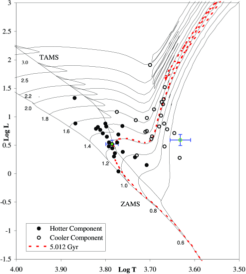
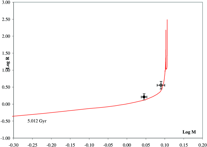
Figure 10: Hotter and cooler components of CF Tuc together with those of the other RS CVn type eclipsing binaries, in which the cooler component is more massive (data from Eker et al. 2008), plotted in the HR diagram (left panel). Comparison between evolutionary models and the physical parameters of CF Tuc in the mass-radius diagram (right panel). The filled and open circle symbols represent the hotter and cooler components in the binaries, respectively. The error bars of the measured quantities are shown by vertical and horizontal lines. Zero Age Main Sequence (ZAMS), Terminal Age Main Sequence (TAMS), the evolutionary tracks and isochrone were taken from Girardi et al. (2000) for the solar chemical composition. The numbers denote initial masses.

The locations of the components of CF Tuc in the luminosity-effective temperature ($T_{eff}$–$L$, i.e. Hertzsprung-Russell diagram) and the mass-radius ($M$–$R$) planes are shown in Fig. 10. We considered only RS CVn type eclipsing binaries, in which the cooler component is a more massive one, to compare the CF Tuc system with other RS CVn’s. According to these diagrams, while the cooler component has evolved behind the terminal age Main Sequence, the hotter one is still on the Main Sequence, approaching the TAMS. This case predicates that CF Tuc is similar to other RS CVn’s. We compared our observationally determined physical parameters with those inferred from the evolutionary tracks in the HR diagram. The best fit appears at age of 5.012 Gyr for both components. The PARAM program at web page (http://stev.oapd.inaf.it/ lgirardi/cgi-bin/param) based on the Bayesian method of da Silva et al. (2006) gives the CF Tuc age as 5.3 Gyr, which agrees well with our determination.

The orbital period change of the system is interesting and difficult to solve. The $O-C$ data of CF Tuc could be represented either by two abrupt period changes or by a sinusoidal period variation superimposed on a downward parabola. In the first case, there appears to be two sudden period jumps: in 1986 and 1995. The first jump shows a period increase, while the second denotes a period decrease. According to the conservative mass transfer mode, the period increase corresponds to a mass transfer from the less massive to the more massive component. In the case of CF Tuc, since the less massive (primary) component is quite far from filling its Roche lobe, this period increase derived from the first jump can not be explained by the mass transfer mechanism. If we take into account the representation of $O-C$ sinusoidal variation superimposed on a parabola; the downward parabola indicates the highest rate of period decrease among the CAB systems. However, since CF Tuc is a detached system, we do not expect direct mass transfer between the components. Therefore, another possible explanation could be a mass loss by stellar wind from the subgiant component. Since the active, subgiant component fills $\sim 89\%$ of its Roche lobe, if a large amount of escaping mass by stellar wind transfers to the primary one, the remaining amount of escaping mass would leave the system. To check this hypothesis, the H$\alpha$ and CaII H & K spectra of the system were examined. Since the RVs of H$\alpha$ and CaII H & K emission features follow the orbital motion of the secondary (cooler) component, these emission features should come from chromospheric and/or coronal layers of that component. From the large width of the H$\alpha$ emission line profile, we estimate turbulent velocities to be up to 200 kms^-1. Such velocities well support our hypothesis that the emission features originate in the circumstellar material.

The sinusoidal form of the orbital period variation was considered as an apparent change and interpreted in terms of the light-time effect due to an unseen component in the system. The large amplitude ($\sim$0.04 day) and small period ($\sim$18 years) of the sinusoidal form of the $O-C$ diagram give quite a large value (2.7 $M_{\sun}$) for the minimum mass of the hypothetical third body. The observed systemic velocity variation and Hipparcos intermediate astrometric data of CF Tuc partially support the hypothesis of the existence of a third body in the system. If such a third body were a main-sequence star, it would be a blue dwarf of a late-B spectral type. However, neither new high-resolution spectroscopic observations nor photometric analysis show any evidence to confirm the presence of such a star. Additionally, we could not expect such a young star as the binary system is much older. Therefore, the hypothetical third body must make a negligible optical contribution to the total light. With this mass, it could be either a massive neutron star (NS) or a black hole (BH). In the case of the companion being a compact object, the question is, can we see it, i.e. in X-rays? CF Tuc was observed by Franciosini et al. (2003) and they detected X-ray photons with energies of one keV in quiescence and a few keV during the flares. This soft X-ray emission was identified as being released in the corona of the magnetically active component. A young NS should give much higher X-ray emission, and an isolated NS would produce a termal X-ray emission of 40-100 keV (Trümper (2005)). The progenitor of the NS must be a B-type star which evolves fast through the Main Sequence, within 100-500 million years, depending on the mass. The newborn NS would have a temperature of 10^7-8 K and could be detected in X-rays. However, assuming the triple system has been formed at the same time and not via a capture, the NS would have enough time to cool down to a much lower temperature. According to the NS models, after 10⁷ years, the NS temperature would be only 10⁵ K. The other possibility, if either a NS or a BH is the third component, could be the accretion luminosity when matter is being accreted onto this object. In fact, a black hole can be seen only through its accretion effects. Due to the large distance from the binary system to the companion (4.9AU), the only possibility for accretion would be through a stellar wind from the binary. Even though CF Tuc has the higher rate of stellar wind among CAB binaries, at the third body separation only a tiny fraction of mass lost by the active component could be accreted, as such accretion is much less efficient than that through the Lagrangian point. We shall estimate the rate according to the formula given by Frank et al. (2002). Taking $\delta M$ = $3.38\times 10^{-7}$ $M_{\sun}$/yr, separation of 4.93 AU, mass of the accreting object to be 3 $M_{\sun}$ and derived radius and mass of the secondary star, we calculated the accretion luminosity to be about $L_{acc}=3.4\times 10^{34}$ erg/s. Such a value is comparable to the quiescent luminosities of NSXN and BHXN (Narayan et al. (2002)) and quiescent low-mass X-ray binary transients (Lasota (2000)). If the third companion is a NS with such a luminosity it should be observed in X-rays, unless the efficiency of the mass transfer to the primary is more efficient than we have assumed. If the companion is a BH, which has no surface, a significant fraction of mass could be lost below the event horizon, instead of being converted into hard photons. Also, if the accretion onto the BH is spherical and not through a bow shock, as considered above, it could be less efficient as well. However, the factors describing this efficiency are within a huge range, between $10^{-8}$ to $10^{-1}$ (Frank et al. (2002), Shapiro (1974), Shapiro (1973), Petrich at al. (1989)) and strongly model dependent (i.e. rotation of the BH, magnetic field, speed of the BH or the accreted material). Concerning the efficiency of the accreting matter being converted into photons, this factor could be in the same range. If the factors are in the lower end, then the existence of a BH as the third companion in CF Tuc in not impossible, though unlikely, as the possibility of its observation may fall below the detection limit and the light time effect would be the only evidence of its existence.

Another explanation of the orbital period sinusoidal variation could be the Applegate mechanism. However, the Applegate model with $M_{s}$=0.1$M$, $\Omega_{dr}=\Delta\Omega$, and $\Delta L_{RMS}=0.1L$ cannot explain the rate of orbital period change observed in CF Tuc.

The last possibility, we can consider, would be a spurious sine term which may not repeat in the future. The observed light curves have strong asymmetries which can affect accuracy of the minima times determination. In some cases, these asymmetries are so large that secondary minima can not even be easily recognized. Therefore, some spurious $O-C$ residuals may come from the asymmetries of the light curve. For instance, Budding and Zeilik (1995) found an approximate 6 year magnetic cycle, considering that these light curve asymmetries were caused by maculation effects. Therefore, we conclude that only future observations can reveal the true nature of the observed period changes. If they are caused by a companion BH, this will be the closest black hole to the Earth.

9 Acknowledgements

This study is related to the Southern Binary Project of the Astrophysics Research Centre at Çanakkale Onsekiz Mart University, the Carter National Observatory, and the Mt John University Observatory in New Zealand. It also forms part of the PhD thesis of D. Doğru and was supported by Çanakkale Onsekiz Mart University Research Foundation under grant no. 2007/55. We thank Prof. John Hearnshaw for granting use of the observing facilities at Mt John University Observatory. We also thank J. L. Innis for making his data available. D. Doğru thanks Professor Edwin Budding and Dr. Hasan Ak for their useful comments and suggestions. Discussions with M. Balucinska-Church and J.-P. Lasota were greatly appreciated. We also thank the anonymous referee for the comments which helped us to improve the quality of this paper.

References

- Anders et al. (1999) Anders G. J., Coates D. W., Thompson K., Innis J. L., 1999, MNRAS, 310, 377
- Applegate (1992) Applegate J. H., 1992, ApJ, 394, 17
- Balona (1987) Balona L. A., 1987, SAAOC, 11, 1
- Bakış et al. (2005) Bakış V., Erdem A., Budding E., Demircan O., Bakış H., 2005, Ap&SS, 296, 131
- Bakış et al. (2006) Bakış V., Budding E., Erdem A.,Bakış H., Demircan O., Hadrava P., 2006, MNRAS, 370, 1935
- Biazzo et al. (2006) Biazzo K., Frasca A., Marilli E., Henry G. W., Soydugan F., Erdem A., Bakis H., 2006, IBVS, 5740
- Bradstreet and Steelman (2002) Bradstreet D. H., Steelman D.P., 2002, AAS, 201, 7502
- Budding and McLaughlin (1987) Budding E., McLaughlin E., 1987, Ap&SS, 133, 45
- Budding et al. (1990) Budding E., Zeilik M., 1990, in İbanoğlu C., ed., Proceedings of the NATO Advanced Study Institute on Active Close Binaries, Kluwer Academic Publishers, Dordrecht, The Netherlands, Boston, p.831
- Budding and Zeilik (1995) Budding E., Zeilik M., 1995, Ap&SS, 232, 355
- Budding et al. (2002) Budding E., Lim J., Slee O. B., White S. M., 2002, NewA, 7, 35
- Budding et al. (2009) Budding E., İnlek G., Demircan O., 2009,MNRAS, 393, 501
- Catalano et al. (2000) Catalano S., Rodono M., Cutispoto G., Frasca A., Marilli E., Marino G., Messina S., 2000, In NATO Science Series C: Mathematical and Physical Sciences, 544, 687
- Claret et al. (1995) Claret A., Díaz-Cordovés J., Gimenez A., 1995, A&AS, 114, 247
- Coates et al. (1983) Coates D. W., Halprin L., Sartori P. A., Thompson K., 1983, MNRAS, 202, 427
- Coates et al. (2000) Coates D. W., Thompson K., Innis J. L., 2000,IBVS, 5007
- Collier et al. (1981) Collier A. C., Hearnshaw J. B., Austin R. R.D., 1981, MNRAS, 197, 769
- Collier et al. (1982) Collier A. C., Haynes R. F., Slee O. B., Wright, A.E., Hiller, D.J., 1982, MNRAS, 200, 869
- Cutispoto and Leto (1997) Cutispoto G., Leto G., 1997, A&AS, 121,369
- da Silva et al. (2006) da Silva L., Girardi L., Pasquini L. etal., 2006, A&A, 458, 609
- Diaz-Cordoves et al. (1995) Díaz-Cordovés J., Claret A., Gimenez A., 1995, A&AS, 110, 329
- Donati et al. (1997) Donati J.-F., Semel M., Carter B. D., Rees D. E., Collier C. A., 1997, MNRAS, 291, 658
- Eker et al. (2008) Eker Z., Ak N. F., Bilir S., Doğru D., Tüysüz M., Soydugan E., Bakış H., Uğraş B., Soydugan F., Erdem A., Demircan O., 2008, MNRAS, 389, 1722
- Erdem et al. (2007a) Erdem A., Soydugan F., Doğru S. S., Özkardeş B., Doğru D., Tüysüz M., Demircan O., 2007a, NewA, 12, 613
- Erdem et al. (2007b) Erdem A., Doğru S. S., Bakış V., Demircan O., 2007b, AN, 328, 543
- Erdem et al. (2009) Erdem A., Budding E., Soydugan E., Soydugan F., Doğru S. S., Doğru D., Tüysüz M., Dönmez A., Bakış H., Kaçar Y., Çiçek C., Eker Z., Demircan O., 2009, NewA, 14, 109
- ESA (1997) ESA, 1997, The Hipparcos and Tycho Catalogues, ESA SP-1200. ESA, Noordwijk
- Fekel et al. (1985) Fekel F. C., Hall D. S., Africano J. L., Gillies K., Quigley R., Fried R. E., 1985, AJ, 90, 2581
- Franciosini et al. (2003) Franciosini E., Pallavicini, R., Tagliaferri G., 2003, A&A, 399, 279
- Frank et al. (2002) Frank J., King A., Raine D., 2002, Accretion Power in Astrophysics, 3rd edition, Cambridge University Press, p75
- Frasca et al. (1998) Frasca A., Marilli E., Catalano S., 1998, A&A, 333, 205
- Frasca et al. (2000) Frasca A., Freire Ferrero R., Marilli E., Catalano, S., 2000, A&A, 364, 179
- Frasca et al. (2005) Frasca, A., Biazzo, K., Catalano, S., Marilli E., Messina, S., Rodono M., 2005, A&A, 432, 647
- Frasca et al. (2008) Frasca A., Biazzo K., Taş G., Evren S., Lanzafame A. C., 2008, A&A, 479, 557
- Girardi et al. (2000) Girardi L., Bressan A., Bertelli G., Chiosi C., 2000, A&AS, 141, 371
- Hadrava (1995) Hadrava P., 1995, A&AS, 114, 393
- Hadrava (1997) Hadrava P., 1997, A&AS, 122, 581
- Hearnshaw and Oliver (1977) Hearnshaw J. B., Oliver J. P., 1977, IBVS, 1342
- Hearnshaw et al. (2002) Hearnshaw J. B., Barnes S. I., Kershaw G. M., Frost N., Graham G., Ritchie R., Nankivell G. R., 2002, ExA, 13, 59
- Hilditch (2001) Hilditch R. W., 2001, An Introduction to Close Binary Stars, Cambridge University Press, p. 292
- Huang (1963) Huang Su-Shu, 1963, ApJ, 138, 471
- Innis et al. (2003) Innis J. L., Coates D. W., Thompson K., Thompson R., 2003, IBVS, 5444
- Innis et al. (2007a) Innis J. L., Coates D. W., Kaye T. G., 2007a,OEJV, 65
- Innis et al. (2007b) Innis J. L., Coates D. W., Kaye T. G., 2007b,PZ, 27
- Kürster and Schmitt (1996) Kürster M., Schmitt, J. H. M. M.,1996, A&A, 311, 211
- Lasota (2000) Lasota J.-P., 2000, A&A, 360, 575
- Lucy (1967) Lucy L. B., 1967, ZA, 65, 89
- Marino et al. (2001) Marino G., Catalano S., Frasca A., Marilli E., 2001, A&A, 375, 100
- Narayan et al. (2002) Narayan R., Garcia M.R., McClintock J.E., 2002, in The Ninth Marcel Grossmann Meeting, ed. V. G. Gurzadyan, R. T. Jantzen, & R. Ruffini (Singapore: World Scientific Publishing), 405
- Olah et al. (1992) Oláh K., Budding E., Butler C. J., Houdebine E. R., Gimenez A., Zeilik M., 1992, MNRAS, 259, 302
- Olah et al. (1998) Oláh K., Marik D., Houdebine E. R., Dempsey R. C., Budding E., 1998, A&A, 330, 559
- Petrich at al. (1989) Petrich, L.I., Shapiro S.L., Stark R.F., Teukolsky S., 1989, ApJ, 336, 313
- Popper and Jeong (1994) Popper D. M., Jeong, Y.-C., 1994, PASP, 106, 189
- Pravdo et al. (1996) Pravdo S. H., Angelini L., Drake S. A., Stern R. A., White, N. E., 1996, NewA, 1, 171
- Randich et al. (1993) Randich S., Gratton R., Pallavicini R., 1993, A&A, 273, 194
- Ribas et al. (2002) Ribas I., Arenou F., Guinan E. F., 2002, AJ, 123, 2033
- Richards and Albright (1999) Richards M. T., Albright G. E., 1999, ApJS, 123, 537
- Rucinski and Duerbeck (1997) Rucinski S. M., Duerbeck H. W., 1997, PASP, 109, 1340
- Rucinski (1969) Rucinski S. M., 1969, AcA, 19, 245
- Shapiro (1973) Shapiro S.L., 1973, ApJ, 185, 69
- Shapiro (1974) Shapiro S.L., 1974, ApJ, 189, 343
- Skuljan and Wright (2007) Skuljan J., Wright D., 2007, ”HRSP Hercules Reduction Software Package”, vers. 3, Univ. Canterbury, New Zealand
- Strassmeier et al. (1999) Strassmeier K. G., Serkowitsch E., Granzer Th., 1999, A&AS, 140, 29
- Strassmeier et al. (2008) Strassmeier K. G., Bartus J., Fekel F. C., Henry G. W., 2008, A&A, 485, 233
- Thompson et al. (1991) Thompson K., Coates D. W., Anders G. PASAu, 1991, 9, 283
- Tonry and Davis (1979) Tonry J., Davis M., 1979, A&J, 84, 1511
- Trümper (2005) Trümper J., 2005, Proc. IAU Symposium No. 232, ”Scientific Requirements for Extremely Large Telescopes”, 236
- van Leeuwen (2007) van Leeuwen F., 2007, A&A, 474, 653
- Wilson and Devinney (1971) Wilson R. E., Devinney E. J., 1971, ApJ, 166, 605
- Zasche and Wolf (2007) Zasche P., Wolf M., 2007, AN, 328, 928
- Zhang and Gu (2008) Zhang L.-Y., Gu S.-H., 2008, A&A, 487, 709
- Zombeck (1990) Zombeck M. V., 1990, Handbook of Astronomy and Astrophysics, Second Edition (Cambridge, UK: Cambridge University Press)