Detailed analysis of an endoreversible fuel cell : Maximum power and optimal operating temperature determination

Abstract

Producing useful electrical work in consuming chemical energy, the fuel cell has to reject heat to its surrounding. However, as it occurs for any other type of engine, this thermal energy cannot be exchanged in an isothermal way in finite time through finite areas. As it was already done for various types of systems, we study the fuel cell within the finite time thermodynamics framework and define an endoreversible fuel cell. Considering different types of heat transfer laws, we obtain an optimal value of the operating temperature, corresponding to a potentially maximum produced electrical power. Finally, two fundamentals results are obtained : high temperature fuel cells could extract more useful power from the same quantity of fuel than low temperature ones with lower efficiencies. Thermal radiative exchanges between the fuel cell and its surrounding have to be avoided so far as possible, because of their negative effects on optimal operating temperature value.

Keywords : Fuel cell, heat engine, efficiency, finite time thermodynamics, entropy, endoreversibility.

1 Introduction

The fuel cell (FC) is usually described as a system that directly converts into electricity the chemical energy provided by a process considered as a combustion [1]. Since it extracts a fraction of useful work from the energy provided by a fuel and a combustive, it could then be also viewed as a particular type of engine. Thereby, as any other engines and according to the second law of thermodynamics, all the provided chemical energy could not be converted into a useful form and a heat quantity is always rejected by the FC to its surrounding. The minimum thermal energy released, corresponding to the maximum produced work, is rejected by a reversible fuel cell (RFC) with no internal production of entropy [2, 3]. In order to include the FC into the finite time thermodynamics framework, we demonstrate in the present study the equivalence between RFC and the Carnot heat engine (CHE), system that extracts the maximum useful work from a given heat quantity.

As it was highlighted by Chambadal [4] and Novikov [5] and later by Curzon and Ahlborn [6], a reversible heat engine can only operate in exchanging heat as an infinitely slow process and therefore can not produce any practical useful power. In fact, energy or mass transfers during finite durations or across finite areas are sources of entropy and leads to a decrease of whole system performances. Taking into account these irreversibilities in the analysis and optimization of system performances is the scope of the finite time thermodynamics[7] (FTT), also called finite dimensions optimal thermodynamics[8] (FDOT). A system producing entropy only because of irreversible exchange processes with its surrounding is usually qualified as endoreversible [9, 10]. The concept of endoreversibility has been successfully applied to a large scale of systems, including different types of engines [11, 12], heat pumps [13], chemical systems [14], distillation devices [15], or pneumatic actuators [16].

As any other type of energy converters, the FC has to reject its own generated heat flux across finite areas or during finite times and can not produce any useful power when being entirely reversible. Indeed, to provide electrical work, a FC, even reversible, has to release the heat produced by chemical process. To be possible, this exchange must be based on a finite temperature difference that produces entropy. Hence, considering a finite thermal conductance between a FC and its surrounding, the Gibbs energy variation, usually sufficient to assess its performances, is then not the only parameter influencing efficiency and quantity of useful work produced. Taking into account the same limitations as for other systems, the FC could be considered as an endoreversible system, producing entropy only in rejecting heat flux in the ambiance [3]. Relevant design and optimization methods of thermodynamical machines, derived from FDOT, could then be applied to theses particular systems [8].

In this article, we study and carry out the performances (produced work and energy efficiency) of an endoreversible fuel cell (EFC) considering different types of heat exchange laws (linear or not). We highlight the existence of an optimal operating temperature and discuss results dealing with different types of hydrogen fuelled FC. Even if the present work focuses on EFC, a similar analysis could be applied to a real, i.e. irreversible FC housing internal productions of entropy.

2 The endoreversible fuel cell

2.1 Reversible fuel cell and Carnot heat engine

Let us consider an open and steady state system operating at constant temperature $T$ and pressure $p$ and housing the followed exothermic chemical reaction :

$$\sum_{j\in{\cal R}}\nu_{j}\cdot A_{j}\to\sum_{k\in{\cal P}}\nu_{k}\cdot A_{k}$$ (1)

with $A_{i}$ the chemical species and $\nu_{i}$ their corresponding stoichiometric coefficients. ${\cal R}$ and ${\cal P}$ are respectively the groups of reactants and products of reaction both considered as ideal gases. Besides molar quantities of reactants and products, it is assumed that the whole system exchanges work $W$ and heat $Q$ with its surrounding.

Considering a system (drawn on Fig. 1) noted 1 like e.g. a fuel cell, which directly converts into work the chemical energy provided by reaction (1), the energy and entropy balances are respectively :

$$\delta W_{1} =-\Delta h(T)\cdot{\rm d}\xi-\delta Q_{1}$$ (2)

$$\delta_{\rm i}S_{1} =\Delta s({\bf p},T)\cdot{\rm d}\xi+\frac{\delta Q_{1}}{T}$$ (3)

with $\Delta h$ and $\Delta s$ respectively the variations of enthalpy and entropy through reaction (1), $\delta Q_{1}$ the exchanged heat quantity, $\delta_{\rm i}S_{1}$ the internal production of entropy, $\bf p$ the vector of the partial pressures of both reactants and products and $\xi$ the reaction progress coordinate defined by :

$${\rm d}\xi=\left(-\frac{{\rm d}N_{j}}{\nu_{j}}\right)_{j\in{\cal R}}=\left(\frac{{\rm d}N_{k}}{\nu_{k}}\right)_{k\in{\cal P}}$$ (4)

Combining (2) and (3), the variation of produced work can be expressed as :

$$\delta W_{1} =-\Delta h(T)\cdot{\rm d}\xi+T\cdot(\Delta s({\bf p},T)\cdot{\rm d}\xi-\delta_{\rm i}S_{1})$$

$$=-\Delta g({\bf p},T)\cdot{\rm d}\xi-T\cdot\delta_{\rm i}S_{1}$$ (5)

with $\Delta g$ the variation of the Gibbs energy $g$ for chemical process (1).

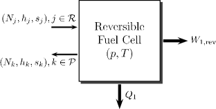
Fig. 1: Schematic diagram of system $1$

Logically, the maximum value of work $\delta W_{1}$ will be produced by a reversible system, i.e. with no internal production of entropy ($\delta_{\rm i}S_{1}=0$) :

$$\delta W_{1,{\rm rev}}=-\Delta g({\bf p},T)\cdot{\rm d}\xi$$ (6)

Dividing this provided work by the reaction progress, we can express the molar reversible work $w_{\rm rev}$ as :

$$w_{1,{\rm rev}}=\frac{\delta W_{1,{\rm rev}}}{{\rm d}\xi}=-\Delta g({\bf p},T)$$ (7)

that corresponds to the quantity of useful energy provided by a reversible system for one mole of consumed chemical reactants. The energy efficiency $\eta$ will be defined as the fraction of useful energy $w_{1}$ on consumed energy, e.g. for the considered reversible system [1] :

$$\eta_{1,{\rm rev}}=\frac{w_{1}}{-\Delta h(T)}=\frac{\Delta g({\bf p},T)}{\Delta h(T)}$$ (8)

Regarding to a real FC, the RFC would be characterised by the absence of overpotentials which are direct results of internal production of entropy [17]. The well known polarization curve i.e. the voltage vs. current produced by the FC should then be replaced by a constant value of voltage, equal to the equilibrium one.

Let us consider now an other system, noted $2$ and drawn on Fig. 2, that produces only heat from chemical reaction (1), which is used as a hot source of a Carnot heat engine (CHE).

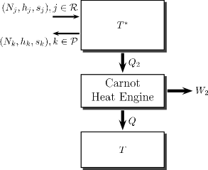
Fig. 2: Schematic diagram of system $2$ feeding a CHE.

First and second laws applied to this combustion system gives :

$$0 =-\Delta h(T)\cdot{\rm d}\xi-\delta Q_{2}$$ (9)

$$\delta_{\rm i}S_{2} =\Delta s({\bf p},T)\cdot{\rm d}\xi+\frac{\delta Q_{2}}{T^{*}}$$ (10)

with $T^{*}$ the temperature of the chemical process. Supposing it reversible ($\delta_{\rm i}S_{2}=0$) and combining (9) and (10), we obtain the temperature $T^{*}$, sometimes called entropic temperature [18] or equilibrium temperature [19] :

$$T^{*}({\bf p},T)=\frac{\Delta h(T)}{\Delta s({\bf p},T)}$$ (11)

This temperature corresponds to the one reached by a combustion process as (1) and both consuming and rejecting reactants and products at temperature $T$. Supplying a Carnot engine operating between temperatures $T$ and $T^{*}$ with heat $\delta Q_{2}$ produced by previous ideal combustion system, we can produce a work quantity [2, 3] :

$$\delta W_{2,{\rm rev}} =\delta Q_{2}\cdot\eta_{2}=\delta Q_{2}\cdot\left(1-\frac{T}{T^{*}({\bf p},T)}\right)=\underbrace{-\Delta h(T)}_{=q^{*}}\cdot{\rm d}\xi\cdot\left(1-\frac{T\cdot\Delta s({\bf p},T)}{\Delta h(T)}\right)$$

$$=-\Delta g({\bf p},T)\cdot{\rm d}\xi$$ (12)

It can be seen that $w_{1,{\rm rev}}=w_{2,{\rm rev}}$ and $\eta_{1,{\rm rev}}=\eta_{2,{\rm rev}}$ and finally concluded on the thermodynamical equivalence of both reversible systems [3], i.e. of RFC and CHE. Indeed, system $2$ is defined as a burner (housing an exothermic chemical reaction) associated to a Carnot engine that producing work. Efficiency $\eta_{2}$ of the whole system is the one of a classical ideal heat engine.

Hence, a RFC could be viewed as a CHE operating with a heat source at temperature $T^{*}$ and a cold sink at its own temperature $T$ (see Fig. 3a).

2.2 Endoreversible fuel cell

As originally demonstrated by Chambadal [4] and Novikov [5], an entirely reversible engine can exhange thermal energies only in a infinitely slowly process and finally can not produce any useful power. Practically, heat transfer can not occur across finite exchange areas in an isothermal way and a finite difference of temperature is necessary to allow rejection of produced heat. In presented our model on Fig. 3b, the FC operates at temperature $T$ in an ambiance at the cold temperature noted $T_{c}$.

Fig. 3: Equivalent heat engines of (a) reversible fuel cell (RFC) and (b) endoreversible fuel cells (EFC).

Rejected molar heat quantity, noted $q$ is now a function of temperatures $T$ and $T_{c}$. De Vos [12] showed that different heat transfer laws could be applied to this system. We will define the general heat transfer law as :

$$q(T,T_{c})=k_{n}\cdot(T^{n}-T_{c}^{n})$$ (13)

where $k$ is equivalent to a thermal conductance (usually defined as a product of heat transfer coefficient and heat transfer area), but divided by reaction progress as precedently did for molar work of relation (7). $n$ is an integer representative of the type of heat transfer law. Then, the heat exchange process will be called linear if $n=1$ and nonlinear if $n>1$.

The equivalent heat engine of Fig. 3b being internally reversible (i.e. endoreversible), its entropy balance is :

$$\frac{q^{*}(T)}{T^{*}({\bf p},T)}=\frac{q(T,T_{c})}{T}$$ (14)

with $q^{*}(T)=-\Delta h(T)$ the heat delivered by an equivalent hot heat source (Fig. 2). Combining (12), (13) and (14), the molar work becomes :

$$w=q(T,T_{c})\cdot\left(\frac{T^{*}({\bf p},T)}{T}-1\right)=k_{n}\cdot(T^{n}-T_{c}^{n})\cdot\left(\frac{T^{*}({\bf p},T)}{T}-1\right)$$ (15)

and related energy efficiency :

$$\eta=1-\frac{T}{T^{*}({\bf p},T)}=\eta_{1,{\rm rev}}$$ (16)

Considering expression (15) of the molar work $w$, three cases have to be considered :

1. If $T=T_{c}$, according to equation (13), no heat quantity can be exchanged and then $q=T\cdot\Delta s=0$ (see Fig. 3a). Therefore, molar variation of entropy $\Delta s$ is null and chemical process can not occur. Thereby, the whole system can not produce any useful work and $w=0$.

2. If $T$ increases, it can reach its maximum value, noted $T_{\max}$, that corresponds to an equality between the operating temperature and the entropic one, i.e. root of the following function :

   $$f(T)=T-T^{*}({\bf p},T)$$ (17)

   This situation leads to the vanishing of Gibbs energy variation :

   $$-\Delta g({\bf p},T_{\max})=0$$ (18)

   and to $w=0$, according to (7).

3. If $T_{c}<T<T_{\max}$, the work $w$ is a continuous and positive function of $T$ which could be maximized.

Unlike other endoreversible engines [8], that are usually supposed to operate with independent values of hot and cold temperatures, relationship (15) (i.e. the molar produced work) depicts a non linear link between entropic and operating temperatures, $T^{*}$ and $T$. This situation corresponds to an equivalent heat engine whose value of the hot source temperature is a function of the cold sink one. Consequently, the maximum power corresponding temperature could not be given as the usual geometric mean of high and low temperatures [20] $\sqrt{T_{c}\cdot T_{\max}}$. However, the optimal temperature $\widehat{T}$ still corresponds to a maximum value of $w$ :

$$\widehat{T}=\arg\max_{T}\left(w(T)\right)$$ (19)

This relationship will be optimized by a Newton numerical algorithm using $\sqrt{T_{c}\cdot T_{\max}}$ as an initial point which turns out to be a good approximation (see Fig. 6).

3 Hydrogen fuel cell

As a practical example, let’s consider the case of an endoreversible fuel cell (EFC) operating in consuming hydrogen as fuel. Chemical reaction (1) is :

$${\sf H}_{2}+1/2\cdot{\sf O}_{2}\to{\sf H}_{2}{\sf O}$$ (20)

The surrounding temperature is fixed for example at $T_{c}=298,15\,{\rm K}$. Thanks to experimental correlations published by the NIST [21], we have represented in Fig. 4 the evolution of the entropic temperature $T^{*}$ vs. reduced temperature for pure oxygen as combustive :

$$\theta=(T-T_{c})/(T_{\max}-T_{c})$$ (21)

Corresponding maximum temperature for pure ${\sf O}_{2}$ is $T_{\max}(x_{{\sf O}_{2}}=1)\simeq 4\,310\,{\rm K}$.

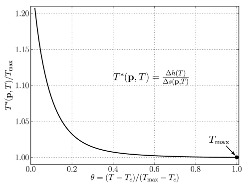
Fig. 4: Entropic temperature $T^{*}$ of relation (11) regarding to the fuel cell (FC) operating one $T$ for pure ${\sf O}_{2}$ as combustive ($x_{{\sf O}_{2}}=1$).

Using air as combustive leads to a similar curve, but with $T_{\max}(x_{{\sf O}_{2}}=0,21)\simeq 3\,884\,{\rm K}$. Dot at the end of curve represents the maximum temperature, corresponding to $\theta=1\Rightarrow T^{*}=T_{\max}$. Using relation (8) and (16), energy efficiencies for some pure oxygen and air as combustive are represented on Fig. 5, with values of coordinate $\theta$ based on maximum temperature with pure oxygen $T_{\max}(x_{{\sf O}_{2}}=1)$.

It can be observed on Fig. 5 a quasi linear decrease of $\eta$ with the operating temperature $T$, leading to a zero value for $T=T_{\max}$ with pure oxygen as combustive. Energy efficiency corresponding to air consumption reach zero at is own value of $T_{\max}$, less than the one of pure oxygen. Range of $\theta$ values does not start at zero because of the possible liquid water formation that can occur below $100^{\circ}{\rm C}$.

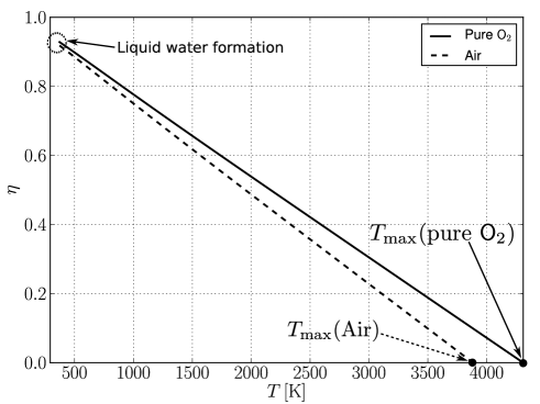
Fig. 5: Energy efficiencies $\eta$ of RFC (relation (8) and (16)) fed by pure ${\sf O}_{2}$ (full line) and air (dashed line) as combustive. Minimum values of $\eta$ for both cases corresponds to respective values of $T_{\max}$.

3.1 Linear heat transfer law

Considering the molar work (15) produced with linear transfer law ($n=1$), it can be given by :

$$w=k_{1}\cdot(T-T_{c})\cdot\left(\frac{T^{*}({\bf p},T)}{T}-1\right)=k_{1}\cdot(T^{*}({\bf p},T)-T)\cdot\left(1-\frac{T_{c}}{T}\right)$$ (22)

That corresponds to the work produced by a Carnot heat engine (CHE) operating between temperatures $T_{c}$ and $T$ and consuming some molar heat $q=k_{1}\cdot(T^{*}({\bf p},T)-T)$. Numerical results are drawn on Fig. 6.

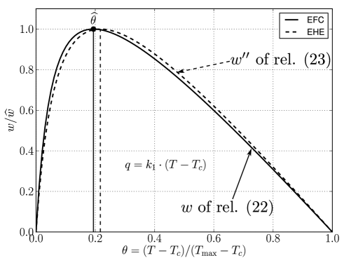
Fig. 6: Reduced molar work $w/\widehat{w}$ vs. $\theta$ with the finite conductance (13) for RFC and for an endoreversible heat engine (EHE) operating between constants temperatures $T_{c}$ and $T_{\max}$.

We have presented in continuous line (curve $1$) the evolution of reduced work $w/\widehat{w}$ vs. reduced operating temperature $\theta$ of relation (21). $\widehat{w}$ is the maximum value of $w$ regarding to temperature $T$. The second dashed line (curve $2$), corresponds to the case where hot temperature is supposed constant and equal to the highest one $T_{\max}$ and where expression of the molar work $w^{\prime\prime}$ corresponds to those of an usual endoreversible heat engine (EHE) :

$$w^{\prime\prime}=k_{1}\cdot(T_{\max}-T)\cdot\left(1-\frac{T_{c}}{T}\right)$$ (23)

This engine is represented on Fig. 3b by replacing variable high temperature $T^{*}$ by the constant one $T_{\max}$. In this particular case, it is easy to show that :

$$\frac{\partial w^{\prime\prime}}{\partial T} =k_{1}\cdot\left(\frac{T_{c}\cdot T_{\max}}{T^{2}}-1\right)=0$$

$$\Rightarrow\widehat{T}=\sqrt{T_{c}\cdot T_{\max}}$$ (24)

and the optimal operating temperature $\widehat{T}$ also leads to a maximum work :

$$\widehat{w}=k_{1}\cdot\left(\sqrt{T_{\max}}-\sqrt{T_{c}}\right)^{2}$$ (25)

and a related energy efficiency :

$$\widehat{\eta}=1-\frac{\widehat{T}}{T_{\max}}=1-\sqrt{\frac{T_{c}}{T_{\max}}}$$ (26)

The difference between curves $1$ and $2$ is a direct consequence of nonlinear link between the entropic temperature $T^{*}$ and the operating one $T$. Therefore, the value of the optimal temperature $\widehat{T}$ corresponding to $w=\widehat{w}$ is lightly modified and actually different from those obtained by a geometric mean (24) of both high and low temperatures. Main results are presented in Table 1.

High temperature	$T^{*}({\bf p},T)$	$T_{\max}$
.$\widehat{T}$	$992\,{\rm K}$	$1\,076\,{\rm K}$
$\widehat{\eta}$	$75,3\%$	$72,3\%$

Table 1: Maximum power operating temperature $\widehat{T}$ and related energy efficiency $\widehat{\eta}$ for variable and constant equivalent high temperatures.

The well used curve $w/\widehat{w}=f(\eta)$ is drawn on Fig. 7 for each endoreversible system. The difference between curves, due to the nonlinearity of $T^{*}$ is here more significant, because of different values of maximum efficiencies. The previous curves are useful for making the difference between low and high-temperatures FC. We have carried out in Fig. 8 the typical range of operating temperatures of protons exchange membrane fuel cells, i.e. $60^{\circ}{\rm C}\leq T\leq 120^{\circ}{\rm C}$ [1]. As previously presented on Fig. 5, a low-temperature fuel cell is characterized with high value of its energy efficiency.

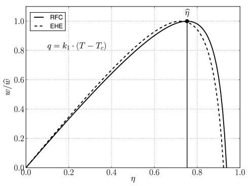
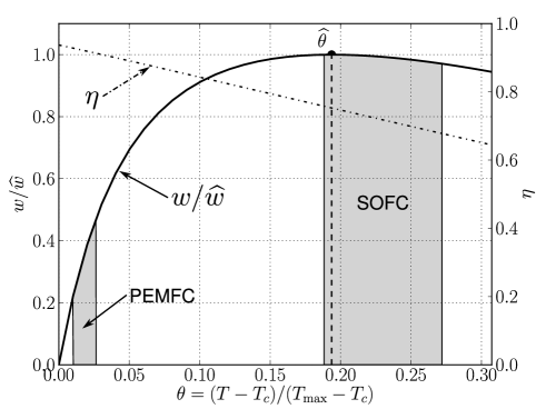
Fig. 7: Reduced molar work $w/\widehat{w}$ regarding to energy efficiency $\eta$ for an EFC and for an EHE operating between $T_{c}$ and $T_{\max}$.

Fig. 8: Reduced molar work and efficiency of different types of FC for air as combustive.

On a first hand, its low temperature difference with surrounding prevents to reject important heat quantity $q$, and according to the Carnot principle, to produce important work $w$ as presented on Fig. 8. On a second hand, high-temperature fuel cells, such as solid oxyde fuel cells (SOFC), can easily evacuate generated thermal power, because of their high temperature differences with the ambiance, and are also able to produce high values of electrical power. On the right part of Fig. 8 is also drawn the typical operating temperature range of SOFC, i.e. $700^{\circ}{\rm C}\leq T\leq 1\,000^{\circ}{\rm C}$. However, this advantage is counterbalanced by a lower energy efficiency, as shown on right part of Fig. 5.

This first result is interesting but does not take into account the difference of heat transfer types between low and high temperature systems. Hence, high temperature heat transfer processes are often driven by radiative effects.

3.2 Nonlinear heat transfer law

Let’s consider now the case of a radiative heat transfer phenomenon ($n=4$) between the FC and the surrounding, we can express the produced molar work as :

$$w=k_{4}\cdot(T^{4}-T_{c}^{4})\cdot\left(\frac{T^{*}({\bf p},T)}{T}-1\right)$$ (27)

As presented on Fig. 9 (full line), the nonlinear heat exchange law leads to a strong increase of the optimal temperature : $\widehat{T}\simeq 2\,910\,{\rm K}$ in the same chemical conditions as previously.

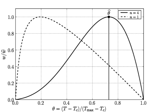
Fig. 9: Evolutions of reduced molar work $w/\widehat{w}$ vs. $\theta$ for $n=4$ (continuous curve) and $n=1$ (dashed curve).

This result could be explained by the fact that the same heat quantity needs a higher value of the temperature difference to be exchanged by a radiative way than thanks to convective phenomenon. The molar heat $q$ corresponding to a maximum produced work could be only released beyond a temperature difference limit higher with some radiative exchanges than with only a convective phenomenon. To make the difference with previous linear case, we have drawn on the same graph the molar work corresponding to the linear heat transfer law (dashed line). The efficiency-work curves of both linear and nonlinear heat transfers laws are presented on Fig. 10.

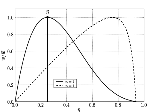
Fig. 10: Evolutions of reduced molar work $w/\widehat{w}$ regarding to energy efficiency $\eta$ with $n=4$ (full line) and $n=1$ (dashed line).

Simultaneously to the increase of the maximum work operating temperature, we can note a strong decrease of related energy efficiency : $\widehat{\eta}\simeq 25\%$. And yet, as presented on Fig. 9, an increase of the operating temperature corresponds to a decrease of its efficiency. Hence, the radiative heat transfer process appears to be unfavourable regarding to EFC performances because it moves forward the optimal operating temperature from those corresponding to convective heat exchange phenomena.

Finally, a relevant thermal management system for high temperature FC will have to minimize radiative losses in order to decrease as much as possible the optimal temperature value $\widehat{T}$ and to get the practical operating temperature $T$ close to it.

4 Conclusions

The formal equivalence between a reversible fuel cell (RFC) and a Carnot heat engine (CHE), both supplied by the same reversible combustion processes, allowed us to describe the former with the finite time thermodynamics approach. The main result is the definition of an endoreversible fuel cell (EFC), operating in a reversible way but exchanging irreversibly heat with its surrounding, through finite thermal conductances. The optimization of the produced work regarding to the fuel cell operating temperature has led to an optimal EFC temperature, numerically calculated for an hydrogen-air reaction for standard conditions of pressure. The influence of the heat transfer law type (linear or not) has been investigated for convective and radiative cases. The last one seems to be unfavourable on the fuel cell performances, because of the increase of the maximum produced work corresponding temperature, compared to linear heat transfer case. At the same time, the efficiency of such system decreasing with temperature, the maximum produced work corresponding efficiency has also strongly decreased. We can conclude on the necessity for a relevant thermal management system to avoid radiative thermal effects and to favour the convective heat exchange phenomena.

The present endoreversible fuel cell is based on an only one thermal finite conductance due to the heat flux exchange with the ambiance. It would be significant to also consider a non reversible chemical reaction, using for example the results of chemical thermodynamics in finite time [22]. In the same way, different types of internal entropy production could be progressively taken into account.

Moreover, design and optimization processes of fuel cell systems have also to take into account the fundamental Carnot principles. The heat flux rejected from the system to the surrounding is fundamental and strongly influences at least the electrical power produced.

Nomenclature

	Acronyms
CHE	Carnot heat engine
EFC	Endoreversible fuel cell
EHE	Endoreversible heat engine
FC	Fuel cell
FDOT	Finite dimensions optimal thermodynamics
FTT	Finite time thermodynamics
RFC	Reversible fuel cell
	Notations
$A$	Chemical species
$g$	Molar Gibbs energy $[{\rm J/mol}]$
$h$	Molar enthalpy $[{\rm J/mol}]$
$\nu$	Stoichiometric coefficient
$p$	Pressure $[{\rm Pa}]$
$\cal P$	Products of a chemical reaction
$Q$	Heat $[{\rm J}]$
$q$	Molar heat quantity $[{\rm J/mol}]$
$\cal R$	Reactants of a chemical reaction
$s$	Molar entropy $[{\rm J/(mol\cdot K)}]$
$\delta_{\rm i}S$	Internal production of entropy $[{\rm J/K}]$
$T$	Temperature $[{\rm K}]$
$W$	Work $[{\rm J}]$
$w$	Molar work $[{\rm J/mol}]$
$\xi$	Reaction progress $[{\rm mol}]$

References

- [1] J. Larminie and A. Dicks. Fuel Cell Systems Explained. Wiley, 2003.
- [2] S. E. Wright. Comparison of the theoretical performance potential of fuel cells and heat engines. Renewable Energy, 29(2):179–195, 2004.
- [3] A. Vaudrey, P. Baucour, F. Lanzetta, and R. Glises. Finite time analysis of an endoreversible fuel cell. In Fundamentals and Developments of Fuel Cell Conference, Nancy, France, December 2008.
- [4] P. Chambadal. Nuclear plants (in french). A. Colin, Paris, 1957.
- [5] I. J. Novikov. The efficiency ot atomic power stations. J. Nuclear Energy, 7(2):125–128, 1958.
- [6] F. L. Curzon and B. Ahlborn. Efficiency of a Carnot Engine at Maximum Power Output. American Journal of Physics, 43:22–24, 1975.
- [7] A. Durmayaz, O. S. Sogut, B. Sahin, and H. Yavuz. Optimization of thermal systems based on finite-time thermodynamics and thermoeconomics. Progress in Energy and Combustion Science, 30:175–217, 2004.
- [8] M. Feidt. Optimal Thermodynamics – New Upperbounds. Entropy, 11:529–547, 2009.
- [9] M. H. Rubin. Optimal configuration of a class of irreversible heat engines. I. Physical Review A, 19(3):1272–1276, 1979.
- [10] M. H. Rubin. Optimal configuration of a class of irreversible heat engines. II. Physical Review A, 19(3):1277–1289, 1979.
- [11] A. De Vos. Efficiency of some heat engines at maximum-power conditions. American Journal of Physics, 53(6):570–573, 1985.
- [12] B. H. Lavenda. The thermodynamics of endoreversible engines. American Journal of Physics, 75(2):169–175, 2007.
- [13] Y. Huang, D. Sun, and Y. Kang. Local stability analysis of a class of endoreversible heat pumps. Journal of Applied Physics, 102(3):034905, 2007.
- [14] M. J. Ondrechen, R. S. Berry, and B. Andresen. Thermodynamics in finite time : A chemically driven engine. Journal of Chemical Physics, 72(9):5118–5124, 1980.
- [15] O. C. Mullins and R. S. Berry. Minimization of Entropy Production in Distillation. Journal of Physical Chemistry, 88(4):723–728, 1984.
- [16] F. Lanzetta, P. Desevaux, and Y. Bailly. Optimization performance of a microfluid flow power converter. International Journal of Fluid Power, 3(3):5–12, 2002.
- [17] Y. Zhao, C. Ou, and J. Chen. A new analytical approach to model and evaluate the performance of a class of irreversible fuel cells. International Journal of Hydrogen Energy, 33(15):4161–4170, 2008.
- [18] A. Laouir, P. Le Goff, and J. M. Hornut. A model mechanism for assessment of exergy: analogic with the balance of a lever. International Journal of Thermal Sciences, 40:659–668, 2001.
- [19] A. De Groot. Advanced exergy analysis of high temperature fuel cell systems. PhD thesis, Delft University of Technology, Delft, Netherlands, 2004.
- [20] A. Bejan. Entropy generation minimization : The new thermodynamics of finite-size devices and finite-time processes. Journal of Applied Physics, 79(3):1191–1218, 1996.
- [21] M. W. Chase. NIST-JANAF Thermochemical Tables. American Institute of Physics, 2000.
- [22] B. Andresen, R. S. Berry, M. J. Ondrechen, and P. Salamon. Thermodynamics for Processes in Finite Time. Accounts of Chemical Research, 17:266–271, 1984.