Designing a Bayesian Network for Preventive Maintenance from Expert Opinions in a Rapid and Reliable Way

Abstract

In this study, a Bayesian Network (BN) is considered to represent a nuclear plant mechanical system degradation. It describes a causal representation of the phenomena involved in the degradation process. Inference from such a BN needs to specify a great number of marginal and conditional probabilities. As, in the present context, information is based essentially on expert knowledge, this task becomes very complex and rapidly impossible. We present a solution which consists of considering the BN as a log-linear model on which simplification constraints are assumed. This approach results in a considerable decrease in the number of probabilities to be given by experts. In addition, we give some simple rules to choose the most reliable probabilities. We show that making use of those rules allows to check the consistency of the derived probabilities. Moreover, we propose a feedback procedure to eliminate inconsistent probabilities. Finally, the derived probabilities that we propose to solve the equations involved in a realistic Bayesian network are expected to be reliable. The resulting methodology to design a significant and powerful BN is applied to a reactor coolant sub-component in EDF Nuclear plants in an illustrative purpose.

Keywords: Bayesian Network, Degradation Process, Log-Linear Model, Expert Opinion, Complexity Reduction, Maintenance.

1 Introduction

Preventive maintenance is considered in a lot of industries because costs due to failures and repairs could be very important. Moreover, since system safety is an important goal for industries, the knowledge of the degradation processes has became essential. Preventive maintenance of a system is taking into account expert knowledge, feedback observations and degradations in order

• to model the system lifetime and to quantify the degradation or failure probability,

• to detect important variables involved in the degradation process and to design maintenance tasks in order to differ or eliminate ageing,

• to quantify the effect of maintenance actions on the system behavior,

• to propose diagnosis and decision help,

• to propose data mining and sensibility analysis.

Bayesian Networks, abbreviated BNs in the following, could be thought of as useful to help engineers to fulfill those purposes of preventive maintenance. BNs provide an efficient way to represent the degradation process of an industrial system or machine. Bayesian Networks are some specific graphical models introduced by Pearl [11], and Lauritzen and Spiegelhalter [10]. Graphical Models introduce a relation between graph and probability theories. The random variables of a probabilistic model are described with the vertices of a graph, where edges describe their dependencies measured with conditional probabilities. A great interest of BNs is to provide an efficient tool for modelling in a simple and readable way the most probable links between events of different nature (expert opinion, feedback experience, …) using conditional independence between random variables. BNs which can also be regarded as a way to introduce randomness in influence diagrams can be expected to be useful for preventive maintenance in the future. The articles of [12] and [13] are recent examples of such maintenance modelling with influence diagrams.

Bayesian Networks, by describing the main conditional probabilities between variables, allow to compute easily the joint probability distribution of all the variables involved in a complex process. However, in order to obtain this joint probability distribution, the number of required probabilities increases exponentially with the number of variables in the model. In the last decade, authors developed algorithms in order to facilitate calculations in graphical models. We can cite the well-known ”junction tree” algorithm (see Lauritzen [10] (1988), Cowell [6] (1999) for instance). Thus many efficient algorithms to deal with computations on more and more complex graphical models are available. These algorithms are included in many software programs like, for instance, the Denmark software Hugin expert [16] and Netica [15] of Norsys Software Corp. If it is essential to develop efficient algorithms to take full advantage of the knowledge contained in graphical models, we must keep in mind that if the knowledge base is poor or badly managed the best algorithm becomes useless (see the introduction section in Cowell et al. [7]). The aim of the present paper is to deal with the practical difficulties encountered when designing a BN for a real maintenance modelling problem. All the ideas we present are motivated and illustrated with the modelling of a nuclear mechanical system degradation with a Bayesian Network.

First, we address the problem of deriving reliable information from experts in a graphical model setting and propose a method to obtain honest probability values in a simple and possibly interactive way from experts knowledge. Then we deal with a second difficulty. In order to compute the joint probability of the variable, the classical BN approach consists of asking for the marginal probabilities of the entry variables and the conditional probabilities of the other variables knowing all the possible combinations between their parents. Owing to the great number of parameters a BN can invovle in practice, it can become a formidable task, and we propose to approximate the graphical model with an unsaturated log-linear model (see for instance [14], chapter 7). This procedure leads to consider that some variables are conditionally independent. In the maintenance modelling context, the experts are asked to provide the marginal probabilities of all the variables and not only of the parent variables as in the classical approach. We choose this method because generally experts can more easily provide such simpler marginal probabilities than conditional probabilities. This strategy leads to a system with more equations than unknown quantities. Thus, it allows us to assess the consistency of the required probabilities. According to Bayes theorem, the properly weighted summation of conditional probabilities of a vertex $N$, knowing a parent vertex, is equal to its marginal probability. After checking the consistency of the given probability values, a feedback procedure is proposed when some inconsistency is encountered, and the experts can choose the reliable given probabilities from their own viewpoint. Thus, the probabilities finally selected to solve the system of $n$ equations with $n$ unknown quantities are expected to be the most reliable ones.

This paper is devoted to present our heuristic strategy to build practically a graphical model in a realistic and relevant way. It is organized as follows. In Section 2, Bayesian Networks models are introduced and a parallel between graphical models and log-linear models which is helpful to reduce the BNs complexity is presented. Section 3 is devoted to the presentation of our methodology to get information from experts in a simple and reliable way. We indicate possible drawbacks of an over restrictive strategy and present ways to remedy these drawbacks. An illustrative application concerning nuclear mechanical system degradation is presented in Section 4 and a short conclusion section ends this paper.

2 Bayesian Networks

Bayesian Networks are powerful graphical models to describe conditional independence and analyze probable causal influence between random variables. In our study, variables are all discrete and most of them are binary. These random variables are represented by the vertices of the graph, and the probable influence between two random variables is represented by an edge between the corresponding vertices. We now give some definitions.

Definition 1

A directed graph is a couple $\mathcal{G}=(V,E)$, where $V=(X_{1},\ldots,X_{n})$ denotes the vertices of the graph and $E=(e_{1},\ldots,e_{m})$ denotes a part of Cartesian product $V\times V$, where $e_{i}$ is called the edges of the graph.

If $(X_{i},X_{j})$ lies in $E$, then this element is called an edge. It is denoted $X_{i}\longrightarrow X_{j}$, $X_{i}$ is called the source and $X_{j}$ the target of the edge. For directed graph, the parents and the children of the vertices are defined as follows:

Definition 2

If a directed edge has source $X_{i}$ and target $X_{j}$, then $X_{i}$ is called the parent of $X_{j}$ and $X_{j}$ is called the son or child of $X_{i}$. The set of the parents of $X_{j}$ is denoted $pa(X_{j})$and the set of children of $X_{i}$ is denoted $ch(X_{i})$.

In a directed graph, the oriented paths are defined as follows:

Definition 3

An oriented path is a set of distinct vertices $X_{i},\ldots,X_{j}$ such that $(X_{k-1},X_{k})$ is an edge for all $k=i+1,\ldots,j$. This path is denoted $X_{i}\longmapsto X_{j}$. A cycle is a path such that $X_{i}=X_{j}$.

Directed graph without cycle are called Directed Acyclic Graphs (DAG). We can now define a Bayesian Network.

Definition 4

A Bayesian Network is

• a set of variables $V$, defining the vertices, and a set of edges between variables $E$,

• each variable has a finite number of exclusive states,

• variables and edges define a directed acyclic graph, denoted $G=(V,E)$,

• for each variable $Y$ with its parents $X_{1},\ldots,X_{n}$, is associated a conditional probability $P(Y|X_{1},\ldots,X_{n})$. When a variable has no parent, the last quantity becomes a marginal probability $P(Y)$.

The denomination ”Bayesian Networks” comes from the well-known Bayes theorem. In a BN, the joint probability can be written as follows (recursive factorization):

$$P(X_{1},\ldots,X_{n})=\prod_{i=1}^{n}P(X_{i}|pa(X_{i})),$$ (1)

where $pa(X_{i})$ is the set of parents of vertex $X_{i}$.

A first problem when designing a BN is to define sensible vertices between the variables involved in the study. This task is made more difficult when numerous variables are available. In our application, in order to deal with this difficulty, we follow a strategy used in Højsgaard [9] to build the structure of the BN. This strategy consists essentially of grouping variables playing analogous roles (see [4]).

In order to draw useful informations from the resulting BN, the knowledge of the joint probability is required. Due to the lack of data, we essentially use experts opinion and we use data when it is possible. However, even with binary variables in Equation (1), it is important to notice that if a vertex has a lot of parent vertices (more than two parents for instance), there are a lot of conditional probabilities to be estimated. In this situation, additional help of experts is needed. But, experts can only give simple probabilities, and it is out of matter to ask them a conditional probability knowing a great number of possible combinations. To overcome this second difficulty, the BN is seen as an unsaturated log-linear model. It is well-known that a BN is always equivalent to an unsaturated log-linear model, where the conditional independences are derived from the moral graph of the BN. Notice that conversely a log-linear model needs that Condition 1 stated below is verified to be representable with a BN. Log-Linear models allow to analyze the relationships between qualitative variables in a contingency table (See Goodman [8], Bishop et al. [1] and Christensen [3]). These models are flexible, currently available in many statistical softwares and have a powerful interpretation in conditional independence terms. With this representation in mind and in order to reduce the number of required conditional probabilities (i.e. the complexity of the BN), some new conditional independences are added.

In an illustrative purpose, consider the BN depicted in Figure 1.

Figure 1: Bayesian Network with four variables.

Figure 1 exhibits the conditional independence of $A$ and $B$ knowing $D$, and of $C$ and $D$ knowing $A$ and $B$. Now consider the associated unsaturated log-linear model:

$$\log(p(a,b,c,d)) = u+u_{A}(a)+u_{B}(b)+u_{C}(c)+u_{D}(d)$$ (2)

$$+ u_{AB}(a,b)+u_{AC}(a,c)+u_{BC}(b,c)+u_{ABC}(a,b,c)$$

$$+ u_{AD}(a,d)+u_{BD}(b,d),$$

with the interaction terms $u$, called $u$-terms, being functions of the cell probabilities of the four-way contingency table. We denote this model $[ABC][AD][BD]$. In this model, $C$ and $D$ are conditionally independent knowing $A$ and $B$. These two representations are strictly equivalent. A possible way to reduce the complexity of the model is to assume that $A$ and $B$ are conditionally independent knowing $C$. It leads to delete the term $u_{ABC}$ in Equation (2). This new unsaturated log-linear model is making sense, but we are facing a problem because it cannot be represented with a BN. This problem can easily be solved by using the following condition (see for instance Christensen [3]).

Condition 1

A log-linear model can be represented by a Bayesian Network if, whenever the model contains all two-order interaction terms generated by a higher-order interaction terms, then the model contains this higher-order interaction terms.

With a more complex BN, for a vertex with a lot of parents, we think that it is impossible to manage all conditional dependences. Thus, to reduce the complexity of a causal BN, we propose to first assume that all $u$-terms, with order greater than two, are equal to zero. It is equivalent to consider conditional independence between parent vertices knowing their son. As this assumption could be too restrictive, in a second stage, we ask the experts to add some higher order associations (three-way interaction terms):The ones they considered useful and reliable. In practice, this additional complexity required by condition (1) to make the log-linear model representable with a BN does not appear to be too important because it is not judicious to model associations of order larger than three. It is important to note that if the expert adds an association, he has to quantify this association by giving the corresponding conditional probabilities.

After this complexity reduction step has been completed, we can design a strategy to extract information from data and experts.

3 Information Extraction Strategy

As seen from Equation (1), the joint probability of a BN can be written in a recursive factorization form. Thus, for all vertices, it is necessary to evaluate the conditional probabilities of the variables knowing their parents. Most of the probabilities are given by expert opinions. The statistician must prepare a questionnaire for the experts. At each probability to be given corresponds a question, written in simple words, without technical stuff. Moreover, the interviews are completed expert by expert. This organization allows to avoid correlations between experts answers.

The main difficulty for a non-statistician expert is to apprehend the conditional probability concept. For instance, let us consider a BN with three binary variables, $S$, $A$ et $C$, respectively smoker, alcoholic, and cancer of throat. Experts are able to give the probability that someone have a cancer of throat knowing that he is a smoker, and the marginal probability to have this cancer. But, the probability that someone has a cancer knowing he is not a smoker is more difficult to evaluate. Most of experts tend to give, for this last probability, the marginal probability to have cancer, considering implicitly that to be a non-smoker is not an information. In this example, experts must be able to give four conditional probabilities, as the probability that someone has a cancer of throat, knowing that he is a non-smoker and a non-alcoholic. This combination is relatively simple for a vertex with two parents, but it seems difficult to give all conditional probabilities with a greater number of parents.

When preparing the questionnaire, it is important not to forget rare events. For instance, let us consider the case of a very reliable component with a probability of default equal to $10^{-6}$. Assume a Bayesian Network with two binary variables: ”default” (yes/no) and ”state” (healthy/failure), where the variable ”state” is a probable consequence of the variable ”default”. In order to compute the joint probability, it is necessary to evaluate the marginal probability of “default” and the two conditional probabilities of the “state” knowing the “default” variable. In this case, it is clearly preferable to query the conditional probability of failure knowing the presence or the absence of default, because both probabilities are significantly different.

The evaluation of all required probabilities, especially conditional probabilities, becomes rapidly an impossible task for experts. Thus, it is of primary importance to give simple rules in order to realize this preliminary step (see [2]). Hereunder, we summarize the rules we have chosen according to the above mentioned considerations.

Rule 1: Query all marginal probabilities. Considering that marginal probabilities are easier to be evaluated, these probabilities are asked even for non input variables. In the classical procedure, only marginal probabilities of input variables are required. However, evaluating all the marginal probabilities does not allow to compute the joint probability. Generally, some conditional probabilities are needed, except if variables are all independent. In the binary case, the number of conditional probabilities is $2^{n}$, where $n$ is the number of parents. It is impossible to evaluate these probabilities as soon the number of parents is greater than three or four.

Rule 2: Query only the conditional probabilities of first order. For instance, let us consider a Bayesian Network with three parent vertices $A$, $B$, $C$ and a son node $D$. For inference, three marginal probabilities are required ($p(A)$, $p(B)$, $p(C)$) and $p(D|ABC)$, corresponding to eight conditional probabilities. in a first approximation, our methodology consists of querying the four marginal probabilities and the following conditional probabilities: $p(D|A)$, $p(D|\bar{A})$, $p(D|B)$, $p(D|\bar{B})$, $p(D|C)$, $p(D|\bar{C})$. These probabilities are usually the simplest ones to give for non-statistician experts. Moreover, one can see that those probabilities involve a lot of redundancies. Thus, this method allows to turn out the incoherences in the expert allocation. Indeed, we have

$$p(D)=\sum_{A}p(D|A)p(A)=\sum_{B}p(D|B)p(B)=\sum_{C}p(D|C)p(C).$$ (3)

In practice, these equations are never exactly verified. The statistician must decide to eliminate some of them. In the example below, one can choose to remove three conditional probabilities. Keeping in mind that conditional probabilities knowing a ”non-event” are difficult to evaluate, thus statistician should remove $p(D|\bar{A})$, $p(D|\bar{B})$ and $p(D|\bar{C})$. However, this rule is not an absolute rule. Hereafter, we propose others rules to decide which probabilities have to be removed.

Rule 3: The most relevant probabilities come from databases. We consider that the feedback experience is more reliable than the expert opinion, especially for conditional probabilities. Moreover, when feedback experience is available, experts based generally their opinion on this feedback experience. In such a situation, some marginal probabilities can be derived wihout too much difficulty, but unfortunately for some variables, with a lot of parent vertices, estimating a conditional probability requires a lot of data.

Rule 4: Favor marginal probabilities provided by the experts. This rule arises from the fact that those probabilities are easier to evaluate, in particular for a non-statistician expert. Thus, it remains to choose one of the conditional probabilities per parent vertex.

For instance, let us consider a Bayesian Network with three vertices as in Figure 2.

Figure 2: BN with two parent vertices.

A possible strategy consists of requiring to which probabilities the expert is more confident. However, in most cases, the choice is very restricted. Indeed, let us suppose that for the BN in Figure 2 where $A$ is a three-level variable, the expert give probabilities displayed in Table 1.

$P(C)=0.25$
$P(C|A=0)=0.05$	$P(A=0)=0.33$
$P(C|A=1)=0.25$	$P(A=1)=0.66$
$P(C|A=2)=0.30$	$P(A=2)=0.01$

Table 1: Example of probabilities given by expert.

From Table 1, it is possible to compute the probability of $C$:

$$P_{calc}(C)=0.05*0.33+0.25*0.66+0.30*0.01=0.183,$$

which is different of the probability given by the expert. Assume now that, in order to remove this gap, the expert decides to evaluate the last conditional probability from an algebraic calculus. It leads to the new conditional probability

$$P_{calc}(C|A=2)=\frac{0.25-0.05*0.33-0.25*.66}{0.01}=6.85!$$

This anomaly comes from the fact that the expert changes the conditional probability which has the lowest weight, namely the weight corresponding to the marginal probability of the parent vertice. Moreover, the highest conditional probability $P(C|A=1)$ with weight of $P(A=1)=0.66$ is equal to the marginal probability and the other conditional probability $P(C|A=0)$ with a significant weight $P(A=0)=0.33$ is rather low. Thus, to remove the difference between the two marginal probabilities (between $0.183$ and $0.25$), the conditional probability is strongly increased and exceeds one …

Rule 5: It is more convenient to change conditional probabilities with large weights, if those probabilities are significantly different of the corresponding marginal probability.

In the previous example, the application of rule 5 gives

$$P_{calc}(C|A=1)=\frac{0.25-0.05*0.33-0.30*0.01}{0.66}=0.3492$$

which replace the previous value of $0.25$. Note here that the ranking of the three conditional probabilities has changed. To preserve the ranking and the ratio between the conditional probabilities, we can change all conditional probabilities by keeping the ratio between the given probabilities.

Assume now that an expert gives the probabilities displayed in Table 2.

$P(C)=0.05$
$P(C|A=0)=0.01$	$P(A=0)=0.33$
$P(C|A=1)=0.03$	$P(A=1)=0.66$
$P(C|A=2)=0.05$	$P(A=2)=0.01$
$P(C|B=0)=0.10$	$P(B=0)=0.10$
$P(C|B=1)=0.03$	$P(B=1)=0.90$

Table 2: Another example of probabilitiesgiven by an expert.

The marginal probability can be seen as a convex combination of the conditional probabilities, where the weights are the marginal probabilities of the vertices parents. Thus, in the fourth line of Table 2, the conditional probability is equal to the marginal probability, $P(C|A=2)=P(C)$. Moreover, two other conditional probabilities ($P(C|A=0)$ and $P(C|A=1$) are strictly lower than the marginal probability. Thus, the weight of the conditional probability $P(C|A=2)$, namely $P(A=2)$ must be equal to one. In this particular case, we propose to change the marginal probability of $C$. The probability $P(C)$ can be computed from the two vertices parents

$$P^{A}_{calc}(C) = 0.029,$$

$$P^{B}_{calc}(C) = 0.037.$$

The first probability is not a convex combination of the conditional probabilities of $C$ knowing $B$, i.e. $0.0029\notin[0.03;0.10]$. Thus, the second computed probability is to be preferred, and the same rules as previously defined are observed in order to change one of the conditional probabilities of $C$ knowing $A$.

Finally, it is possible to keep ratio between conditional probabilities by solving the following linear program

$$\min_{0\leq x\leq 1}|P(C)-\sum_{i=1}^{3}k_{i}xP(A=i)|$$

where $k_{i}$ represents the ratio between the conditional probabilities given by experts.

In the last example, if no assumption is made on conditional independence, experts must give the conditional probability of $C$ knowing $A$ and $B$. Thus, we apply the same rules for these conditional probabilities, keeping in mind that we asked first the conditional probabilities of $C$ knowing $A$ and the conditional probabilities of $C$ knowing $B$. If the number of parents vertices is $n$ and if associations with order greater than three are considered, the conditional probabilities can be computed by induction.

4 Application

The above described methodology has been applied to build a BN for a sub-component of a Reactor Coolant Pumps, observed on the French Nuclear Plants. In this context, the choice of the system and the experts is crucial. First, the study must concern a system which the experts considered significant for the safety of the whole industrial entity (here a nuclear plant). Moreover, the system must be well-known by the experts and the availability of the experts to build the structure of the graph must be a significant criterion, because this kind of project could be long and demanding and need many meetings. It is important to underline that the statistician have to play a role of mediator. He has to clearly define the goal of the project and describe the various powerful possibilities of this kind of model.

In the present case, the main goal of the study was to model the system degradation with a BN in order to define the most appropriate maintenance tasks and to evaluate the possible effects of this maintenance tasks. In what follows we sketch the important points of this study according to the above described modelling and indicate the practical interest of this study.

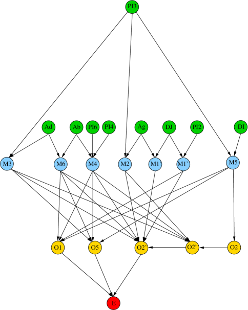
Figure 3: Bayesian Network of a system degradation process.

In Figure 3, we present a BN, built from experts opinions of the research and development division of EDF according to the strategy described in [9]. This Bayesian Network contains 22 discrete variables, 17 variables are binary and the other five ones have three modalities. According to the strategy of Højsgaard [9], variables have been divided in four sets: environmental variables $\mathcal{A}=\{PI3,Ad,Ab,PI6,PI4,Ag,DJ,PI2,DI\}$, degradation variables $\mathcal{M}=\{M1^{{}^{\prime}},\-M1^{{}^{\prime\prime}},M2,M3,M4,M5,M6\}$, observation variables $\mathcal{O}=\{O1,O2,O2^{{}^{\prime}},O2^{{}^{\prime\prime}},O5\}$ and finally the variable of interest: the state of the system ($E$).

From the Bayesian Network presented in Figure 3, the likelihood of the model is given by

$$p(U) = p(Ab)p(Ad)p(Ag)p(PI2)p(PI3)p(PI4)p(PI6)p(DI)p(DJ)$$ (4)

$$\times p(M1^{{}^{\prime}}|Ag,DJ)p(M1^{{}^{\prime\prime}}|DJ,PI2)p(M2|Ag,PI3)P(M3|Ad,PI3)$$

$$\times p(M4|Ab,PI4,PI6)p(M5|DI,PI3)p(M6|Ad,Ab)$$

$$\times p(O1|M1^{{}^{\prime\prime}},M4,M5,M6)p(O5|M3,M4,M5,M6)p(O2|M5)$$

$$\times p(O2^{{}^{\prime\prime}}|M2,M3,M4,M6,O2)$$

$$\times p(O2^{{}^{\prime}}|M1^{{}^{\prime}},M1^{{}^{\prime\prime}},M2,M3,M4,M6,O2^{{}^{\prime\prime}})p(E|O1,O5,O2^{{}^{\prime}}).$$

Inference from this BN requires the estimation of 381 probabilities in Equation (3). Now, since few data from feedback experience are available, experts must give a lot of probabilities and especially a lot of conditional probabilities. For instance, for the node $O2^{{}^{\prime}}$, the classical approach requires to evaluate 192 conditional probabilities, a formidable task to deal with. Thus, in order to make the inference step feasible, we regard the BN as an unsaturated log-linear model, where all association terms of order greater than two are constrained to be zero. As stated above, this point of view is equivalent to assume that all parent nodes (variables) are conditionally independent knowing their sons. To evaluate all the probabilities needed for the computation of the joint probability, we proceeded by induction from the environmental variables to the variable of interest.

For instance, $p(M6\mid Ab,\;Ad)$ had to be computed in Equation (3). Assuming that $Ad$ and $Ab$ are conditionally independent knowing $M6$, $P(Ab)$, $P(Ad)$, $P(M6)$, $P(M6\mid Ab)$ and $P(M6\mid Ad)$ were needed to compute $P(M6\mid Ab,\;Ad)$.

$$P(M6\mid Ad,Ab) = \frac{P(Ad,Ab\mid M6)P(M6)}{P(Ab)P(Ad)}=\frac{P(Ad\mid M6)P(Ab\mid M6)P(M6)}{P(Ab)P(Ad)}$$

$$= \frac{P(M6\mid Ab)P(M6\mid Ad)}{P(M6)}.$$

The above formula is quite simple since $Ab$ and $Ad$ are conditionally independent knowing $M6$, but $P(M6)$ had to be provided.

In the same manner, to compute $p(O1|M1^{{}^{\prime\prime}},M4,M5,M6)$, by assuming that $M1^{{}^{\prime\prime}},M4,M5,M6$ are conditionally independent knowing $O1$, we get

$$P(O1\mid M1^{{}^{\prime\prime}},M4,M5,M6)=\frac{P(M1^{{}^{\prime\prime}},M4,M5,M6\mid O1)P(O1)}{P(M1^{{}^{\prime\prime}},M4,M5,M6)}$$

$$=\frac{P(M1^{{}^{\prime\prime}}\mid O1)P(M4\mid O1)P(M5\mid O1)P(M6\mid O1)P(O1)}{P(M1^{{}^{\prime\prime}},M4,M5,M6)},$$

with

$$P(M1^{{}^{\prime\prime}},M4,M5,M6)=P(M1^{{}^{\prime\prime}})P(M5)\sum_{Ab}P(M4\mid Ab)P(M6\mid Ab)P(Ab),$$

where $M4$ and $M6$ are not independent, but are conditionally independent knowing $Ab$. Finally, $P(O1\mid M1^{{}^{\prime\prime}},M4,M5,M6)$ could be written

$$\begin{array}[]{l}P(O1\mid M1^{{}^{\prime\prime}},M4,M5,M6)=\\ \displaystyle\frac{P(O1\mid M5)P(O1\mid M1^{{}^{\prime\prime}})P(O1\mid M4)P(O1\mid M6)P(M4)P(M6)}{P(O1)^{3}\sum_{Ab}P(M4\mid Ab)P(M6\mid Ab)P(Ab)}.\end{array}$$

The last example concerns the variable of interest $E$ and the conditional probability $P(E\mid O1,O5,O2^{{}^{\prime}})$:

$$P(E\mid O1,O5,O2^{{}^{\prime}}) = \frac{P(O1,O5,O2^{{}^{\prime}}\mid E)P(E)}{P(O1,O5,O2^{{}^{\prime}})}=$$

$$= \frac{P(O1\mid E)P(O5\mid E)P(O2^{{}^{\prime}}\mid E)P(E)}{P(O1,O5,O2^{{}^{\prime}})}$$

$$= \frac{P(E\mid O1)P(E\mid O5)P(E\mid O2^{{}^{\prime}})}{P(E)^{2}P(O1,O5,O2^{{}^{\prime}})}$$

with

$$P(O1,O5,O2^{{}^{\prime}}) = \sum_{\mathcal{M}}P(O1,O5,O2^{{}^{\prime}}\mid\mathcal{M})P(\mathcal{M})$$

$$= \sum_{\mathcal{M}}P(O1\mid\mathcal{M})P(O5\mid\mathcal{M})P(O2^{{}^{\prime}}\mid\mathcal{M})P(\mathcal{M})$$

$$= \sum_{\mathcal{M}}P(O1\mid pa(O1))P(O5\mid pa(O5))P(O2^{{}^{\prime}}\mid pa(O2^{{}^{\prime}})P(\mathcal{M})$$

and

$$P(\mathcal{M}) = \sum_{\mathcal{A}}P(\mathcal{M}\mid\mathcal{A})P(\mathcal{A})$$

$$= \sum_{\mathcal{A}}\prod_{X\in\mathcal{M}}P(X\mid\mathcal{A})\prod_{Y\in\mathcal{A}}P(Y)$$

$$= \sum_{\mathcal{A}}\prod_{X\in\mathcal{M}}P(X\mid pa(X))\prod_{Y\in\mathcal{A}}P(Y).$$

Using the assumption that all the association terms of order greater than two were null, the likelihood could be computed from all marginal probabilities and conditional probabilities of order one (namely, conditional probability of a variable knowing a unique variable and not a combination of numerous variables). For instance, for the node $O2^{{}^{\prime}}$, the classical approach required 192 conditional probabilities, whereas our method required only seven conditional probabilities.

For the whole BN, in the present application, the number of required probabilities decreased from 381 to 69. Moreover all required probabilities are now easily interpreted and evaluated by the experts. To determine the final probabilities from the evaluations provided by the experts we made use of the rules given in the previous section. It can be noticed that by querying more probabilities that necessary allowed us to choose the most reliable probabilities in a repeated dialog with the experts.

Thus after analyzing the first results on the initial BN, the experts wished to be more precise by adding nine conditional dependences. With this new graphical model, the experts suggested to introduce some carefully selected two-order interactions. After they evaluated the additional probabilities, the same computation rules were applied to lead to a new Bayesian network. The inference on the resulting BN shows that three variables ($Ab$, $Ad$ and $PI3$) appeared to be quite influent on the system degradation.

These results encouraged to add maintenance tasks on those three variables in order to improve the reliability of the system. The maintenance tasks were easily included in the model as new variables of the BN (see [5]) and the experts gave the new conditional probabilities (typically, the probability of an environmental variable knowing a maintenance task) by using the methodology previously described. A new inference from this updated BN allowed to give the effect of the maintenance actions and to simulate a great number of possible strategies.

5 Conclusion

Bayesian Network is a powerful tool to model associations between relevant variables of a problem. This kind of modelling requires the intervention of experts. In this work, we concentrated efforts to provide efficient heuristic methods to get a reliable and meaningful Bayesian network from the practical point of view. First, we applied simple rules to collect information and to design the structure of the graph. Then, we defined simple and coherent methods to evaluate the probabilities that are needed for inference. We gave simple rules in order to keep the more reliable probabilities, required to compute the joint probability of the network. Marginal and conditional probabilities are determined first from operating experience and secondly from expertise. One of the main interests of this work which is detailed in [4] is to propose a strategy avoiding a too heavy and too unstable acquisition of expert information. This strategy is reducing the number of questions to be asked. Moreover it allows to include maintenance actions as new vertices of the BN (see Corset et al. [5]). Thus, the effect of a maintenance action can be predicted, a point which is rather new and of interest.

References

- [1] Y.M. Bishop, S.E. Fienberg, and P.W. Holland. Discrete multivariate analysis. Cambridge, MA : MIT press, 1975.
- [2] C. Chatelain and A. Lannoy. Une application de la technique du réseau bayésien à l’évolution des coûts de maintenance. Technical Report HP-20/00/020/A, EDF, July 2000.
- [3] R. Christensen. Log-Linear Models. Springer Texts in Statistics. Springer-Verlag, New York, 1990.
- [4] F. Corset. Aide à l’optimisation de maintenance à partir de réseaux bayésiens et fiabilité dans un contexte doublement censuré. PhD thesis, Université Joeseph Fourier, Grenoble, 2003.
- [5] F. Corset, G. Celeux, A. Lannoy, and B. Ricard. Bayesian networks as a decision tool in maintenance with expert judgement. In ESReDA 23rd Seminar on Decision Analysis: Methodology and Applications for Safety of Transportation and Process Industries, Delft University, Netherlands, November 18-19 2002.
- [6] R. Cowell. Introduction to Inference for Bayesian Networks. The MIT Press, 1999.
- [7] R.G. Cowell, A.P. Dawid, S.L. Lauritzen, and D.J. Spiegelhalter. Probabilistic Networks and Expert Systems. Statistics for Engineering and Information Science. Springer, 1999.
- [8] L.A. Goodman. The multivariate analysis of qualitative data : interaction among multiple classifications. J. Amer. Statist. Assoc., 65:226–256, 1970.
- [9] S. Højsgaard. Learning structures from data and experts. Mathematics and Computers in Simulation, 42:143–152, 1996.
- [10] S. L. Lauritzen and D. J. Spiegelhalter. Local computations with probabilities on graphical structures and their application to expert systems. J. R. Statist. Soc. B, 50(2):157–224, 1988.
- [11] J. Pearl. Probabilistic Inference in Intelligent Systems. Morgan Kaufmann, San Matteo, California, 1988.
- [12] M. Sachon and E. Pat-Cornel. Delays and safety in airline maintenance. Reliability Engineering and System Safety, 67:301–309, 2000.
- [13] J. Vatn. Maintenance optimisation from a decision theoretical point of view. Reliability Engineering and System Safety, 58:119–126, 1997.
- [14] J. Whittaker. Graphical Models in Applied Multivariate Statistics. Wiley, 1990.
- [15] http://www.norsys.com/download.html.
- [16] http://www.hugin.com/Products_Services/.