Numerical Solution of a nonlinear reaction-diffusion problem in the case of HS-Regime
Abstract.
In this paper, the author propose a numerical method to compute the solution of the Cauchy problem: , the initial condition is a nonnegative function with compact support, . The problem is split in two parts: A hyperbolic term solved by using the Hopf and Lax formula and a parabolic term solved by a backward linearized Euler method in time and a finite element method in space. Estimates of the numerical solution are obtained and it is proved that any numerical solution is unbounded.
1. Introduction
In this paper, we study a numerical method to compute the solution of the Cauchy problem :
| (1.1) |
is a function with compact support, , .
Samarskii et al [10], see also [1], [2], [3], [6], [5], [4] , [9] have obtained theoretical results on this problem. In the case , the numerical solution blows up in finite time and there is no localization (HS-regime) that is .
A numerical method to solve (1.1) has been proposed in the case of S-regime () in [7] and in the case of LS-regime ( [8]. If we denote , in the case of S-regime, is positive while in the case of LS-regime , . The problem is solved by using a splitting method; for that, it is more convenient to work with the function . Problem (1.1) may be written:
| (1.2) |
with .
This problem is split in two parts: a hyperbolic problem which will be solved exactly at the nodes at each time step and allows the extension of the domain and a parabolic problem which will be solved by a backward linearized Euler method which allows the blow up of the solution.
In [7], [8], the convergence of the scheme has been proved in the cases and . It has also been proved that for , the numerical solution blows up in finite time for any initial condition and that its support remains bounded if the initial condition is smaller than a self-similar solution. In the case, any numerical solution is unbounded while for () if the initial condition is sufficiently small, a global solution exists and if for large initial condition, the solution blows up in a finite time. We observe numerically that in any case, the unbounded solution is strictly localized and blows up in one point and that for also, if the initial condition is sufficiently small, a global solution exists.
Here, we generalize this method to the case
An outline of the paper is as follows:
In Section 2, we present the numerical scheme. In Section 3, we obtain estimates of the approximate solution and of its derivative in space. In Section 4, we prove that if , ()) any numerical solution is unbounded
2. Definition of the numerical solution
In order to solve problem (1.2), we separate it in two parts: a hyperbolic problem
| (2.1) |
and a parabolic problem
| (2.2) |
We denote by the time increment between the time levels and and by the approximate solution at the time level . This solution will be in a finite-dimensional space which will be defined below.
Without loss of generality, we can assume that the initial condition is a continous function with a symmetric compact support . Let, the space step is defined by we note and we define the finite dimensional space by
| (2.3) |
For , we note and for any function with compact support , we define its interpolate by and .
The support of the solution will be denoted and will be computed at each time level by solving (2.1).
We denote
(for , denotes the greatest integer less than ), so we get: .
We then define the finite-dimensional space by:
and denote by the Lagrange interpolate in of a function with a compact support in .
The solution at the time level is computed in two steps: knowing , we compute first an approximate solution of (2.1) which will be denoted ; then starting with this intermediate value, we compute an approximate solution of (2.2) at time level .
Then if is the semi-group operator associated with (2.1), we define
The support of this function will be denoted and the interpolate of in will be denoted .
Then starting with , the function is obtained by solving (2.2) with a backward linearized Euler method in time and a -finite element method with numerical integration in space. This function has the same support as .
2.1. Computation of the solution of the hyperbolic problem
The hyperbolic problem is independent of ; we use the same method as in [7] for the case .It is not necessary in this case to use -interpolation on the last interval since there no localization. We use the Hopf and Lax formula which gives explicitely the solution to (2.1) with the starting data at the time level . Here, we simply recall the results obtained in [7]
We define the piecewise constant function by
Let us denote .
Proposition 2.1.
If the following stability condition
| (2.4) |
is satisfied, then the solution of (2.1) is defined by
If , we get
and we get analogous formula at the other end of the support.
2.2. Computation of the parabolic problem
The approximate solution at is now obtained by solving problem (2.2).
We introduce the approximate scalar product on
We define as the solution of the following problem:
| (2.5) |
The second member of (2.2) is splitted in two parts in order to obtain the -estimate of
This equation may be written:
We get immediately the result:
2.3. Properties of the scheme
Lemma 2.3.
If the hypotheses of proposition 2.2 are satisfied, then the following estimate holds:
| (2.7) |
Proof: We get immediately from the Hopf and Lax formula that . If we denote the index such that , we get from (2.2), (2.2), (2.2) that
which proves the lemma.
We deduce the following theorem:
Theorem 2.4.
Under the hypotheses of proposition 2.2, the numerical solution exists at least until the time
| (2.8) |
and the following estimate holds:
| (2.9) |
Proof: This result is proved recurently. It is true for . If we suppose that we have estimate (2.9) at the time level , we get from (2.7) , at the time
or
The inequality (2.9) will be satisfied at the time if :
By using the Taylor formula, we get:
and the inequality (2.3) is satisfied:
Lemma 2.5.
Under the hypothesis of Proposition( 2.2), we have the estimate:
for where is a constant depending on and .
Proof: We have the inequality( [7] ):.
It remains to estimate .
From (2.2), we deduce the following equation satisfied by :
and we have analogous inequalities for .
By using (2.2) for , we can replace in the second member by its expression in function of the values of and and we get:
Let the index such that From the previous equality, we get:
We easily obtain:
and
and we get:
By (2.9), we get easily there exist a positive constant depending on such that
Hence for , we get .
Lemma 2.6.
Under the hypotheses of Proposition (2.2), we have the estimate:
| (2.10) |
for where is a constant depending on and .
Proof: From the properties of the semigroup operator [7], we get: , and by using the equations satisfied by , we obtain:
and we immediately deduce the estimate (2.10).
In this case, since the variation of is not bounded.
3. Blow-up of the solution
In this part, we prove that for the solution blows up in finite time.
3.1. Construction of unbounded solutions
Define the function
We note . If the initial condition is with , we prove that it is possible to choose and in such a manner that with
and then the numerical solution blows up in finite time.
We denote , .
The support of is ; its lenth is increasing with the time.
If , we get .
The support of is with
Since is a symmetric function, it is sufficient to study the case ,.
We get for
for such that since the function is decreasing for and we have:
with .
Hence, we obtain:
with .
Then will be a subsolution of (2.2) if
By using the equality :
this inequality reduces after simplifications to
Noting that with , we get:
and the inequality (3.1) becomes:
By using the equality this inequality reduces to:
If we denote since , the preceding inequality will be satisfied if:
| (3.1) |
From the stability condition, we get:
hence for sufficiently small, we get: and
So the inequality (3.1) will be satisfied if :
Since we introduce the function defined on by :
or
with
A sufficient condition to satisfy (3.1) is:
We have ,
hence we get
But since , we get:
and
So, if the quantity is such that if is sufficiently small, we get .
Let us define , and if , we obtain ; if we obtain:
.
This quantity will be positive if : .
Further, we have:
The solution at the time level exists if , that is
and if , we get:
and will be positive if:
| (3.2) |
The second member is a function of , hence if is fixed such that ,
the inequality (3.2) will be satisfied if is large enough and sufficiently small.
Hence if the initial condition satisfies , and satisfying (3.2), the solution blows up in finite time.
3.2. Blow-up of the solution
Theorem 3.1.
Let The solution of problem (1.2) blows up in finite time.
Proof:Since , there exists such that for such that
So we can choose large enough such that and .
We have and then the solution blows up at time where
.
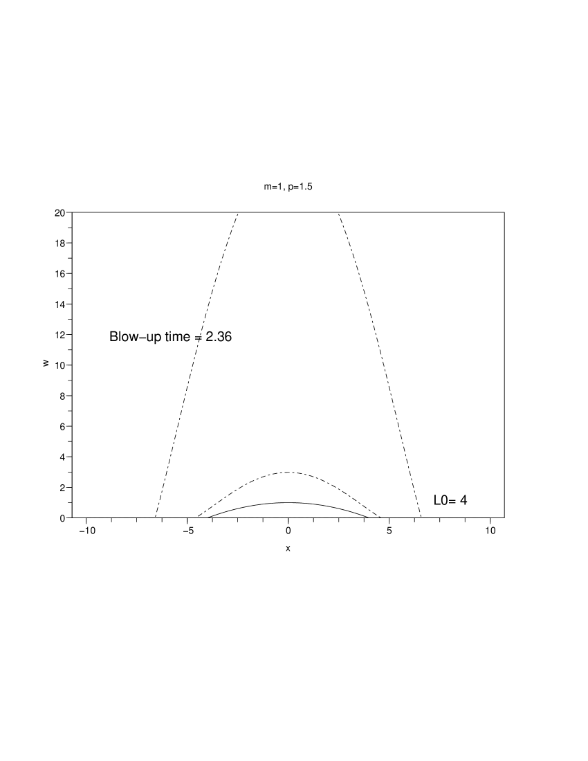
In Fig1, we present the evolution of an initial condition for . The solution blows up in finite time.
References
- [1] C. Bandle and H. Brunner. Blowup in diffusion equations:A survey. J. Comput. Appl. Math., 97:3–22, 1998.
- [2] J. Bebernes and V.A. Galaktionov. On classification of blow-up patterns for a quasilinear heat equation. Differential and Integral Equations, 9(4):655–670, 1996.
- [3] V.A. Galaktionov. On localization conditions for unbounded solutions of quasilinear parabolic equations. Sov.Math.Dokl., 1982.
- [4] V.A. Galaktionov. Best possible upper bounds for blowup solutions of the quasilinear heat conduction equation with source. SIAM J. Math. Anal., 22(5):1293–1302, 1991.
- [5] V.A. Galaktionov. On a blow-up set for the quasilinear heat equation . J. Differential Equations, 101:66–79, 1993.
- [6] V.A. Galiaktonov. Asymptotic behaviour of unbounded solutions of the nonlinear parabolic equation u. Differential Equations (English Translation), 21:751–758, 1985. Differentsial’nye Uravneniya, 21 ,n 7,(1985) 1126-1134.
- [7] A.Y. Le Roux and M.N. Le Roux. Numerical solution of a nonlinear reaction diffusion equation. Journal of Computational and Applied Mathematics, 173:211–237, 2005.
- [8] A.Y. Le Roux and M.N. Le Roux. Numerical solution of a cauchy problem for nonlinear reaction diffusion processes. www-gm3.univ-mrs.fr, 2007.
- [9] P.E. Sacks. Global behavior for a class of nonlinear evolution equations. SIAM J. Math. Anal., 16(2):233–250, 1985.
- [10] A.A. Samarskii, V.A. Galaktionov, S.P. Kurdyumov, and A.P. Mikhailov. Blow-up in Quasilinear Parabolic Equations. Walter de Gruyter, Berlin (English traduction), 1995. Nauka, Moscow(1987), in Russian.