Heterogeneous attachment strategies optimize the topology of dynamic wireless networks

Abstract

In optimizing the topology of wireless networks built of a dynamic set of spatially embedded agents, there are many trade-offs to be dealt with. The network should preferably be as small (in the sense that the average, or maximal, pathlength is short) as possible, it should be robust to failures, not consume too much power, and so on. In this paper, we investigate simple models of how agents can choose their neighbors in such an environment. In our model of attachment, we can tune from one situation where agents prefer to attach to others in closest proximity, to a situation where distance is ignored (and thus attachments can be made to agents further away). We evaluate this scenario with several performance measures and find that the optimal topologies, for most of the quantities, is obtained for strategies resulting in a mix of most local and a few random connections.

I Introduction

The performance of a network is a consequence of three factors — the hardware, the network protocols and the network topology. For some networked systems, like the wireless mesh networks, the topology can be controlled rather easily through the medium access layer, and it is thus practically possible to optimize the topology of the network. In this work, we investigate a scenario of static agents (sensors, individuals with Wi-Fi devices, etc.), embedded in space, joining and leaving the system (so called “churn”). Our scenario is based on the following three assumptions. First, only new agents and neighbors of an agent leaving the network create new links. Second, the power consumption of each agent is, for fairness and practical reasons, to be restricted. Third, the agents are localized with uniform randomness over the unit square. From these starting points, we evaluate different simple attachment strategies to optimize several network-structural quantities, capturing efficiency of communication, scalability and robustness to failure.

Many of the previous studies on topological optimization of wireless networks have concerned static point patterns li:algo , not (as in our study) systems under churn. Nevertheless, these studies form a theoretical backdrop of ours. The simplest approach to connecting wireless agents in the plane is to let all agents within range be connected. Assuming identical agents, one arrives at the Unit Disc Graph model of wireless networks ruhrup:performance . Maintaining and routing information in a network with this architecture, however, is a waste of power and memory resources. Many theoretical efforts in this area have been focusing on energy efficient, yet scalable topologies — a seminal work is yao:graph , where the “Yao graph” was proposed. This graph is constructed by connecting each node to its closest neighbor in $k$ equiangular sectors. It has several topological features, such as (almost surely) full connectivity and scalable power consumption, which are desirable for wireless networks. Subsequent studies have proposed improved proximity graphs, with localized construction algorithms more ruhrup:performance ; li:sparse ; li:power or less liu:distributed_topo_control ; kuhn:beyond_udg ; li:topo similar to the Yao graph, and studied general features of minimum power topologies rodoplu:minimum_energy ; watten:dist . Our approach is from a slightly different angle, taking more inspiration from the recent complex network literature mejn:rev ; doromen:book ; eugster:from_epi . These works discuss how dynamic properties of networks in general (including communication performance in technological networks) are related to network structure (how the observed network topology differs from what is expected in a unconstrained random network model). This approach lends itself naturally to analyzing topics like point-to-point communication, and data distribution scenarios in large, to some extent random, systems. In this work we evaluate the possibility to optimize network topology in the case when connections cost power, and consequently, due to limitations of energy storage, agents maintaining long connections can keep only a limited number of neighbors.

In the next section, we give a precise description of the problem and our proposed attachment models and discuss related practical issues. We evaluate the proposed models considering a large set of performance measures in Section III. Finally, Section IV concludes our work.

II Preliminaries

II.1 Problem statement

We consider a set $V$ of $N$ agents spread out on the unit square. In our numerical study, the spatial distribution will be uniformly random, but generalizing to other point patterns is straightforward. At every time step, one random agent leaves the system and a new one enters (at a random coordinate). The agents form a graph with bi-directional connections. For two agents $i$ and $j$ at coordinates $\mathbf{r}_{i}$ and $\mathbf{r}_{j}$ to be connected it costs both agents a power consumption of $p(i,j)=|\mathbf{r}_{i}-\mathbf{r}_{j}|^{\delta}$ ($2\leq\delta\leq 4$) liu:distributed_topo_control . In this work we focus on the limit $\delta=2$. We assume the agents to be selfish and homogeneous in the sense that no agent $i$ accept a higher power-consumption $\sum_{j\in\Gamma_{i}}p(i,j)$ (where $\Gamma_{i}$ is $i$’s neighborhood), than $P_{\mathrm{max}}$. This also ensures scalable, total power consumption. We also assume a lower power limit $P_{\mathrm{min}}$, such that while an agent consumes less power than $P_{\mathrm{min}}$, it will attempt to create new links in the network (unless creating any new link would result in a larger power consumption than $P_{\mathrm{max}}$). Thus $P_{\mathrm{min}}$ represents a minimal investment all agents agree to contribute with to the system. Based on these precepts, we try to find simple attachment strategies (rules for agents to select other agents to link to) that optimize various objective functions. To assess unperturbed network performance, we measure the following quantities (that will be discussed in greater detail in the Section III).

• Connectivity. We measure connectivity as the fraction of time steps when the graph is completely connected. This quantity should, in any functioning network, be very close to one. Except when we explicitly study this quantity, we tune the parameters so that the graph is almost always connected.

• Power consumption and power efficiency. We consider the value of aggregate power consumption and the power efficiency (the ratio of power consumption across the shortest multihop path and a direct link). Low values are desirable for efficient communication.

• Diameter. $d_{\mathrm{max}}=\max_{i,j\in V}d(i,j)$. Where $d(i,j)$ is the distance (the number of links in the shortest path) between $i$ and $j$.

• Average distance $\bar{d}=\frac{2}{N(N-1)}\sum_{i,j\in V}d(i,j)$. The overhead in communication time grows with distance; thus, a small diameter and short average distance are desirable.

• Spectral gap, $E$ — the difference between the largest and second largest eigenvector of the adjacency matrix. This is an approximate measure of the link expander property hoory:xpndr that embodies several desirable properties for wireless networks (little redundancy, high robustness, efficient broadcast, etc.).

Since we do not construct an optimal network each time step, only update the network incrementally, it is important to monitor the effect of churn. Indeed, this problem is similar to another important aspect — the robustness to failure and we measure it by the two quantities:

• The change, $\Delta d_{\mathrm{max}}$, of the diameter as a random node is deleted from the network.

• The change, $\Delta\bar{d}$, of the average distance.

We aim at finding simple, local attachment strategies optimizing these quantities — local in the sense that each agent follows its own rules.

II.2 Model definition

We will investigate two models, both having in common that they interpolate between situations where the power budget is spent only on short-range connections, to a situation where connections are made at random regardless of location. At every time step, a random agent $i^{\prime}$ is removed along with its connections $\Gamma_{i^{\prime}}$ and a new agent added. This can cause both the new agent and $\Gamma_{i^{\prime}}$ to have power consumptions below $P_{\mathrm{min}}$. All agents $i$ with $P(i)<P_{\mathrm{min}}$ try to attach to new agents $j$. If adding a link $(i,j)$ would make either $P(i)$ or $P(j)$ larger than $P_{\mathrm{max}}$, or if $(i,j)$ already is a link in the graph, the link is not added. These properties are the same for both models. The differences between the models are:

• Model A. With probability $q_{A}$, attach $i$ to the closest possible agent, otherwise attach $i$ to a random agent.

• Model B. There are two kinds of agents — a fraction $q_{B}$ of them always attach to the closest possible agent, the rest attaches to a random agent.

Note that in the limits $q_{A}=q_{B}=0$ and $q_{A}=q_{B}=1$, the models are identical.

II.3 Practical considerations

The main assumption of the proposed models is that the power consumption of an agent $i$ is proportional to $\sum_{j\in\Gamma_{i}}p(i,j)$, where $\Gamma_{i}$ is the set of agents connected to $i$ and $p(i,j)=|\mathbf{r}_{i}-\mathbf{r}_{j}|^{\delta}$. This requires transmission power control to be implemented at the agents. We motivate the assumption on power consumption as follows. First, once the network topology is defined, and if the traffic load in the network is balanced, both unicast and broadcast routing scenarios are likely to have a similar average usage of the connections. (In a situation with heterogeneous agents of very different capacities and network positions, this would not hold.) Second, considering dynamic power control, the required transmission power depends on the transmission channel characteristics. In systems designed for tolerable outage probability it is sufficient to consider the distance-dependent path loss to set the required transmission power rodoplu:minimum_energy . Finally, we do not consider the energy spent for data reception and processing. These are distance independent additive values and consequently would not change the main conclusions of our study.

For the implementation of the attachment strategies described in Section II.2, the problems of distance-dependent neighbor selection and efficient access control to the shared wireless medium have to be solved.

If the network, for efficient higher layer protocols (like geographic routing takagi:geo ), keeps information about the location of the nodes, then such information can also improve the proposed attachment models. If absolute node location information is not maintained, agents can select neighbors by discovering a given area via beaconing with increasing transmission power (see for example watten:dist for detailed solutions).

The medium access control is responsible for sharing the wireless medium in an efficient way. TDMA, CSMA and mixed solutions are usually proposed, depending on the expected network load loscri:mac . Since the interference region of a connection depends on the distance of the transmitting and receiving agent, the construction of an optimal access control scheme is not trivial in the addressed scenario. An optimal access control should take the attachment model into account and schedule most local and random connections separately. The efficiency of the medium access control can potentially affect the network performance, which calls for extended future studies.

III Numerical results

In this section we will discuss results from our numerical simulations. Unless otherwise stated, we use $10^{6}$ time steps for equilibration and $10^{6}$ time steps for measuring averages.

Figure 1: The average degree $\bar{k}$ for our models. (a) shows results for model A, (b) for model B. $P_{\mathrm{max}}=2P_{\mathrm{min}}=2$, and (c) shows the size scaling for $q_{A}=q_{B}=0$. The line in (c) represents growth proportional to $N^{1/2}$. Standard errors are smaller than the symbol size.

III.1 Average degree

Many of the performance measures, like connectivity and network diameter are directly related to the number of connections the agents maintain — that is, the average degree. Since the number of connections an agent can maintain in the considered case depends on the attachment strategy, we start investigating the average degree.

We can derive approximate results for the two extreme cases, $q_{A}=q_{B}=0$ and $q_{A}=q_{B}=1$. For $q_{A}=q_{B}=0$, each agent tries to connect to the closest available neighbor. Assuming that all connections can be made and that the agents are uniformly spread out (so that the number of agents $n_{r}$ within distance $r$ from point is $\pi r^{2}N$), this means that the power consumption to attach to agents within a distance $R$ is

$$\int_{0}^{R}r^{\delta}2\pi rN\,\mathrm{d}r=\frac{2\pi N}{2+\delta}R^{2+\delta}~{}.$$ (1)

For a given minimal power $P_{\mathrm{min}}$ the number of agents within reach is

$$\pi N\left(\frac{2+\delta}{2\pi N}P_{\mathrm{min}}\right)^{2/(2+\delta)}\in O(N^{\delta/(2+\delta)})~{}$$ (2)

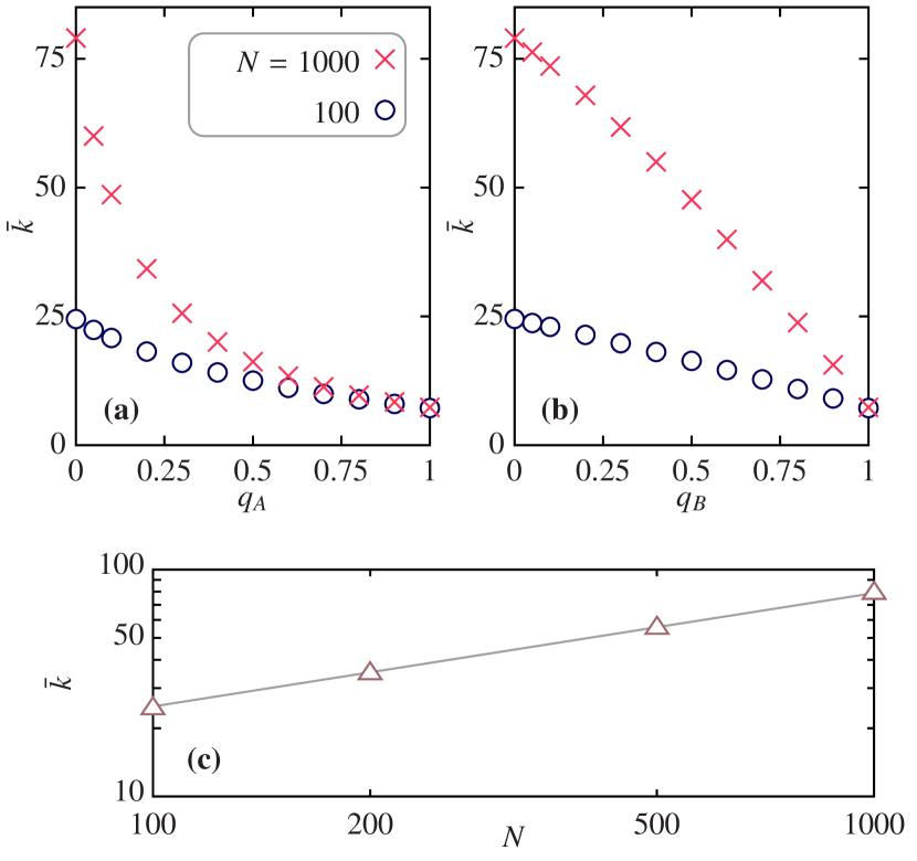
or in other words, for $\delta=2$ the average degree $\bar{k}\in O(N^{1/2})$. This relationship is confirmed in Fig. 1. In the opposite limit, $q_{A}=q_{B}=1$, all agents attach to others at random. Since the average distance to another, random, agent is independent of $N$, then so is $\bar{k}$ (which also can be seen in Fig. 1). The functional forms of $\bar{k}$, as functions of $q_{A,B}$ are strikingly different. Even if $\bar{k}$ itself is not a performance measure, it affects network performance; therefore a stable response to the parameter values is beneficial. We note that the curves for Model B has a smaller slope for small values of $q_{B}$, whereas Model A has larger magnitude of the derivative when $q_{A}$ is close to zero.

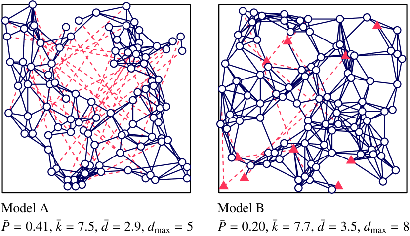
The key to understanding the difference in degree between the two model is the observation that the number of long-range links is much lower in Model B than in Model A (Fig. 1). $P_{\mathrm{max}}$ controls the power consumption so that it is relatively similar for both models. With the power consumption constrained, more power-expensive, random links leads to a sparser network. So why does Model A have more random links? New links are added until the power consumption reaches above $P_{\mathrm{min}}$. Since the steps in power consumption are larger when a random connection is added, the chance that the last added link, for Model A, is by random attachment is larger than $q_{A}$. For model B, on the other hand, the chance the last added connection is long range is $q_{B}$, so $\bar{k}$ will be a linear combination of the $q_{B}=0$ and $q_{B}=1$ limits. Therefore, for $q_{A}=q_{B}$ the number of long-range edges and the power consumption will be higher for Model A than Model B. These mechanisms can also be understood from our example figure, Fig 2. To make this figure readable we use smaller values of $N$ and $P_{\mathrm{min}}$ than in the rest of the paper. We also use a relatively large $P_{\mathrm{max}}$, making the $\bar{k}$ more similar between the models at the expense of a more different power consumption. From this figure we see the difference in number of long-range links even more pronounced than in Fig. 1.

From Fig. 1(a) and (b) we learn that the degree can be controlled continuously by the model parameters $q_{A}$ and $q_{B}$. It would maybe be convenient for the discussion if we could neglect the model parameters and investigate the models in terms of some basic network quantity like $\bar{k}$. However, such an approach is complicated by the fact that, for $q_{A,B}<1$, the average degree also depends on $N$ (see Fig. 1(c) and the above discussion). Moreover, the size scaling of $\bar{k}$ depends on $q_{A}$ and $q_{B}$, going continuously (but with different functional forms) from $\bar{k}\sim N^{1/2}$ for $q_{A}=q_{B}=0$, to size independence for $q_{A}=q_{B}=1$. For this reason we keep the control parameters $q_{A,B}$ as our main independent parameters in this investigation and do not go into details of functional forms when discussing the size dependence of performance measures.

Figure 2: Snapshot of the models with $N=100$, $P_{\mathrm{min}}=0.1$, $P_{\mathrm{max}}=1$, and $q_{A}=q_{B}=0.1$. The dashed lines are formed by random attachment. The triangles in (b) are the agents with a random attachment strategy rather than attachment to the closest other node.

Figure 3: The connectivity is shown as a function of $q_{A,B}$ and $P_{\mathrm{min}}$ (panel (a) and (b)) or $P_{\mathrm{max}}$ for Model A (panel (a) and (c)) and Model B (panel (b) and (d)). The fraction $\varphi$ of time steps when the network is fully connected is measured and displayed as color scales so that the numbers at the color bars correspond to $-\lg(1-\varphi)$, white means that the network is almost always connected. In all panels we set $2P_{\mathrm{min}}=P_{\mathrm{max}}$ and use $N=1000$.

III.2 Connectivity

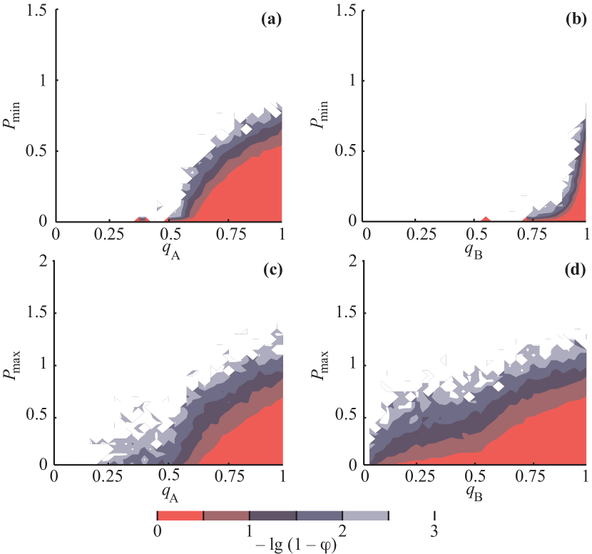
A fundamental functional requirement is that the network should be connected. There is, in principle, nothing that guarantees connectivity in our construction algorithm. We investigate the connectivity, quantified as $\varphi$ — the fraction of time steps when the network is fully connected. Since $\varphi$ is close to one, we rather plot $-\lg(1-\varphi)$ (Fig. 3). The larger are values of the energy limits (both $P_{\mathrm{min}}$ and $P_{\mathrm{max}}$), the better is the connectivity — by consuming more power, the network can always be made connected — a trivial but necessary fact. In the white region of the density plot in Fig. 3, the network is fully connected more than 99.9% of simulation runs ($\varphi>0.999$ and thus $-\lg(1-\varphi)>3$). In the rest of this paper we will (unless stated otherwise) investigate a region of parameter space where the network is almost surely connected — $P_{\mathrm{min}}=1$ and $P_{\mathrm{max}}=2$.

As seen in Fig. 3, a qualitative difference between the two models is that the connectivity of Model B is less dependent on $q_{B}$ than Model A is dependent on $q_{A}$. For a large range of $q_{B}$ (Fig. 3(b)), the network is connected almost regardless of $P_{\mathrm{min}}$. One explanation is the higher degrees of Model B — adding links, increasing the degree, can connect, but not fragment, a network. The connectivity depending on the $P_{\mathrm{max}}$ value (Fig. 3(c) and (d)) shows different tendencies: Model A becomes connected at lower $P_{\mathrm{max}}$-values (and consequently lower $P_{\mathrm{min}}$-values). To explain this feature we evaluate the actual power consumption of the two models in the next section.

Figure 4: Power consumption for the two attachment models A and B as functions of their respective parameters, $q_{A}$ and $q_{B}$. Other parameter values are the same as in Fig. 1. Standard errors are smaller than the symbol size.

Figure 5: The average (per node pair) ratio between the actual consumed power and the power of a direct connection $\rho$ for the two attachment schemes as a function of their respective control parameter. Other parameter values are the same as in Fig. 1. Standard errors are smaller than the symbol size.

III.3 Power consumption

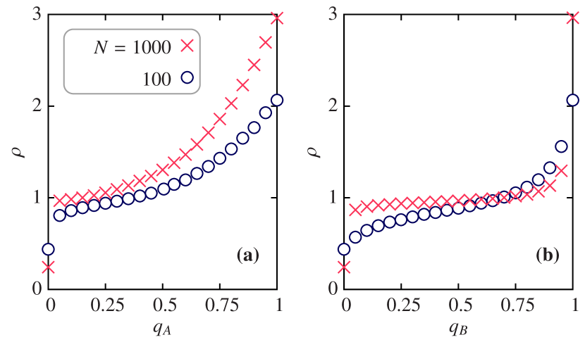
The power consumption of an agent is a stochastic variable in the interval $[0,P_{\mathrm{max}}]$, changing as agents join and leave the network. (While in both models the agents try to allocate at least $P_{\mathrm{min}}$, we have to note that if an agent cannot connect without raising the power consumption over $P_{\mathrm{max}}$, its power consumption will be below $P_{\mathrm{min}}$.) If the average power consumption is higher, so more resources are invested in the infrastructure, one can expect the network properties to improve. Therefore, to better be able to analyze our performance measures, we investigate the level of power consumption. Fig. 4(a) and (b) shows the average power consumption with $P_{\mathrm{min}}=1$ and $P_{\mathrm{max}}=2$. The power consumption maximally fluctuates $\sim 20\%$ and it is always lower for model B. This difference increases with system size for all values except close to $q_{A,B}=1$, meaning that performance advantages for Model A in these limits, especially for larger systems, should be evaluated with this increased power consumption in mind. Or, alternatively, a specific $q_{A}$-value can be translated to a (higher) $q_{B}$-value, corresponding to the same power consumption.

Why is the power consumption higher in Model A? Again, we use Fig. 2 can give an illustration. Above, we explained why, if $q_{A}=q_{B}$, Model A has larger fraction of long-range edges than Model B. Since the steps in power consumption is larger when adding random edges, if a random edge is the last one added, then the power consumption overshoots $P_{\mathrm{min}}$ more. In sum, more randomly added links mean more overshoot and thus higher power consumption.

Power efficiency in multihop networks is often measured by the ratio $\rho$ of actual consumed power to the power needed for a direct connection, averaged over all vertex pairs (scaling like the distance squared):

$$\rho=\frac{1}{{N\choose 2}}\sum_{i<j\in V}\frac{\sum_{(i^{\prime},j^{\prime})\in\pi(i,j)}p(i^{\prime},j^{\prime})}{p(i,j)}$$ (3)

where $\pi(i,j)$ is the set of links forming the shortest path (in number of hops) between $i$ and $j$  ruhrup:performance . If the route between the source and the target is circuitous, $\rho$ might be much larger than one, but if it proceeds in several steps relatively straight towards the target, $\rho$ can be smaller than unity. Indeed, the lower bound of $\rho$ is zero — assume $i$ and $j$, at distance $r$ are connected by a straight path of $n$ equidistant links. Then $p(i^{\prime},j^{\prime})$ for all links along the path is $r^{2}/n^{2}$, so the whole sum in the numerator equals $r^{2}/n$, while the denominator is $r^{2}$, giving a contribution $1/n$ from the node pair $\{i,j\}$ to $\rho$. In Fig. 5 we plot this quantity for Model A and B, and two different network sizes. The $\rho$-curves are monotonically increasing for both sizes and attachment models. Both models have some regions of their parameter space where $\rho<1$, which is the definition for being a power spanner ruhrup:performance . Model B shows lower values of $\rho$ for a large region of its parameter space, which means that shortest path routes are straighter compared to the ones in Model A, a results of the different distribution of long-range random connections.

Figure 6: Distance-related measures for different sizes and parameter $q_{A,B}$ values. Panels (a) and (b) shows the average distance $\bar{d}$ while (c) and (d) shows the diameter $d_{\mathrm{max}}$. Other parameter values are the same as in Fig. 1. Standard errors are smaller than the symbol size.

III.4 Distances

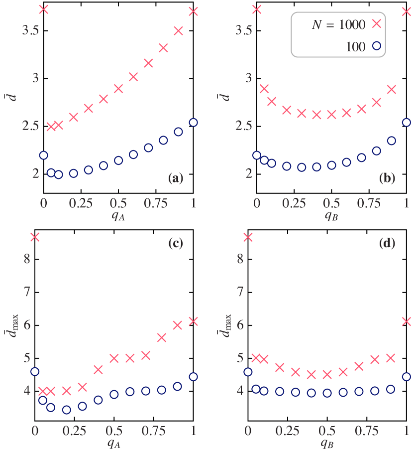
Both for unicast and multicast communication, short distances (in number of hops) are beneficial, as they lead to lower delays gamal:throughput . In Fig. 6 we investigate the average distances and diameter, corresponding to mean and extreme-case connections as a function of the model parameters $q_{A}$ and $q_{B}$. For both Model A and B, and both distance measures, the minima are attained for intermediate values of $q_{A,B}$. In other words, a mix between random and short-range connections optimizes network distances. Furthermore, the minimum occurs for low $q_{A,B}$-values, i.e. with larger proportion short-range connections compared with the random connections. The decreasing distances for $q_{A,B}\approx 0$ can be understood as a “small-world effect” — we only need to introduce a few random links to a regular graph for it to go from algebraic to logarithmic distance scaling wattsstrogatz ; bollobas_chung_88 . The increasing distances for larger $q_{A,B}$-values can be explained by the decreasing average degrees. Comparing Models A and B, we note that Model A gives the smallest distances (both average and maximal). If one increases the degree of a graph by adding links to it, its average distance cannot increase. Similarly, most network models have distances decreasing with the average degree. With that in mind, it is a little surprising that Model A has both shortest distances and smallest average degree. This non-trivial, purely topological effect can only be related to the distribution of longer-range, random links. In Model A, the long-range links are more evenly distributed out between the agents (compared with Model B where, at least one side of the every long-range link belong to one class of nodes). Model A loses this advantage as more random links are inserted in the network, then the average and maximal distances increase together with the decreasing degree according to Fig. 1. Model B has the advantage that it is not as sensitive to $q_{B}$ as model A is to $q_{A}$.

Figure 7: The spectral gap, the difference between the two largest eigenvalues of the adjacency matrix, for model (a) and (b). Other parameter values are the same as in Fig. 1. Standard errors are about the size of the symbols, but omitted for readability.

III.5 Expander property

For multicast and broadcast communication, redundancy is an important topological factor. Imagine a triangle between agents $1$, $2$ and $3$. A broadcast originating from $1$ reaches $2$ and $3$ in two steps. Then, however, the link between $2$ and $3$ is redundant — both $2$ and $3$ already have the packet. If a graph has few such redundancies, it is said to have good expander properties. The usual way of defining this property is via the expansion factor $\Phi$ — the minimum over all subsets $S$, smaller than half the entire vertex set, of the ratio between the size of the neighborhood of $S$ and the size of $S$  ernesto:commu . $\Phi$ is a computationally hard quantity. Instead, we measure the spectral gap $\bar{E}$ — the difference between the leading and second largest eigenvalues of the adjacency matrix, which is known to be a lower bound to $\Phi$ (apart from a factor $2$) hoory:xpndr .

In addition to efficient broadcast communication, large spectral gap also leads to two other desirable network properties. First, it reflects robustness. It is known that if the graph has a large spectral gap one needs to cut many links to split it into two disjoint subnetworks hoory:xpndr . Consequently, the spectral gap is a measure of resilience against a worst-case scenario of an adversary deliberately trying to disconnect different parts of the network our:attack . Second, networks with large spectral gaps are easier to synchronize donetti:sync . This is especially relevant for synchronizing clocks of sensor networks li:sync .

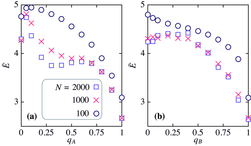
In Fig. 7, we plot the expander coefficient for the two models corresponding to Fig. 6. The best parameter range is for small $q_{A,B}$. In contrast with the distance measures, the maximum $\bar{E}$ for Model B is network size dependent and does not always occur for an intermediate $q_{B}$-value. Model A, on the other hand, has a maximum for small $q_{A}$-values. For both models there is a small $q_{A,B}$ value where $\bar{E}$ is high and stable (indeed accentuated) as the system grows. This stable value is higher for Model A, which indicates that Model A can achieve higher performance than Model B for the same system size. For intermediate $q_{A,B}$-values, $\bar{E}$ seems to converge for Model B, whereas it decreases (roughly) logarithmically for Model A. Because of this, in implementations where the system size is unknown a priori, and the model parameter is hard to control exactly, Model B might be advantageous. Model A also shows a second incipient peak for the larger sizes, much lower than the low-$q_{A}$ peak and probably uninteresting for practical applications.

Figure 8: The expected difference in average distance as a random node is deleted from the network. Panels (a) and (b) shows curves for Model A and Model B respectively. Other parameter values are the same as in Fig. 1. Standard errors are smaller than the symbol size.

III.6 Robustness

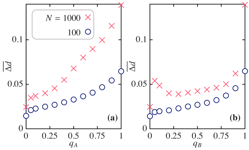
In addition to resilience to worst case attacks measured by the spectral gap, it is desirable that network graphs are robust to random failures. This is, in fact, similar to demand that the turnover of agents should not worsen our objective functions much. To investigate how random failures affect the network we measure $\Delta\bar{d}$ — the difference in average pathlength if a random node is disconnected from the network. From Fig. 8 we can see that this quantity is also optimized at low $q_{A,B}$-values. But in contrast to the behavior of $E$, $q_{A}=0$ is optimal for Model A and a small $q_{B}$ (around $q_{B}=0.2$) is optimal for Model B ($N=1000$). Like other quantities, Model B is less $q_{B}$-dependent than Model A is $q_{A}$-dependent. Both models have similar magnitude of $\Delta\bar{d}$.

IV Summary and conclusions

We have investigated the optimization of network topology of the medium access layer of wireless networks, and found that agents with simple but heterogeneous rules for finding neighbors are capable to form network with shorter average distances, better expander properties and relatively high robustness (compared to random, or Unit Disc Graph approaches). The two models we test have parameters controlling the ratio of long-range interactions. We find that close to (but not at) one end of parameter space (where most connections are short) is the region where optimal topologies exist.

For most score functions — average distance, diameter and spectral gap — our Model A (where agents attach to spatially close others with a probability $q_{A}$, otherwise to random agents) gives better values than our Model B (where there are two classes of agents, one making only short connections, one making only random connections). The good topological properties of Model A are however outweighed by the effect of fast decreasing average degree as $q_{A}$ increases. Model B, on the other hand, has the advantage that its performance is less dependent on the parameter value.

References

- (1) B. Bollobás and F. R. K. Chung. The diameter of a cycle plus a random matching. SIAM Journal on Discrete Mathematics, 1:328–333, 1988.
- (2) L. Donetti, P. I. Hurtado, and M. A. Muñoz. Entangled networks, synchronization, and optimal network topology. Phys. Rev. Lett., 95:188701, 2005.
- (3) S. N. Dorogovtsev and J. F. F. Mendes. Evolution of Networks: From Biological Nets to the Internet and WWW. Oxford University Press, Oxford, 2003.
- (4) A. El Gamal, J. Mammen, B. Prabhakar, and D. Shah. Optimal throughput-delay scaling in wireless networks: part i: the fluid model. IEEE/ACM Trans. Netw., 14:2568–2592, 2006.
- (5) E. Estrada. Communicability in complex networks. Phys. Rev. E, 77:036111, 2008.
- (6) P. T. Eugster, R. Guerraoui, A.-M. Kermarrec, and L. Massoulie. From epidemics to distributed computing. IEEE Computer, 37:60–67, 2004.
- (7) P. Holme, B. J. Kim, C. N. Yoon, and S. K. Han. Attack vulnerability of complex networks. Phys. Rev. E, 65:056109, 2002.
- (8) S. Hoory, N. Linial, and A. Wigderson. Expander graphs and their applications. Bulletin of the American Mathematics Society, 43:439–561, 2006.
- (9) F. Kuhn and A. Zollinger. Ad-hoc networks beyond unit disk graphs. In DIALM-POMC ’03: Proceedings of the 2003 joint workshop on Foundations of mobile computing, pages 69–78, New York, NY, 2003. ACM.
- (10) N. Li and J. C. Hou. Topology control in heterogeneous wireless networks: Problems and solutions. In IEEE INFOCOM 2004, pages 232–243, 2004.
- (11) Q. Li and D. Rus. Global clock synchronization in sensor networks. IEEE Transactions on Computers, 55:214–226, 2006.
- (12) X.-Y. Li. Algorithmic, geometric and graphs issues in wireless networks. Wireless Communications and Mobile Computing, 3:119–140, 2003.
- (13) X.-Y. Li, P. J. Wan, and Y. Wang. Power efficient and sparse spanner for wireless ad hoc networks. In IEEE ICSN, 2001.
- (14) X.-Y. Li, P.-J. Wang, Y. Wang, and O. Frieder. Sparse power efficient topology for wireless networks. In Proceedings of the 35th Annual Hawaii International Conference on System Sciences, pages 3839–3848, 2002.
- (15) J. Liu and B. Li. Distributed topology control in wireless sensor networks with asymmetric links. In Global Telecommunications Conference, 2003.
- (16) V. Loscrı. MAC protocols over wireless mesh networks: problems and perspective. J. Parallel Distrib. Comput., 68(3):387–397, 2008.
- (17) M. E. J. Newman. The structure and function of complex networks. SIAM Review, 45:167–256, 2003.
- (18) V. Rodoplu and T. H. Meng. Minimum energy mobile wireless networks. IEEE Journal on Selected Areas in Communications, 17:1333–1344, 1999.
- (19) S. Rührup, C. Schindelhauer, M. Grünewald, and K. Volbert. Performance of distributed algorithms for topology control in wireless networks. In In 17th International Parallel and Distributed Processing Symposium, page 2003, 2008.
- (20) H. Takagi and L. Kleinrock. Optimal transmission ranges for randomly distributed packet radio terminals. IEEE Transactions on Communications, 32(3):246–257, 1984.
- (21) R. Wattenhofer, L. Li, P. Bahl, and Y. M. Wang. Distributed topology control for wireless multihop ad-hoc networks. In INFOCOM, pages 1388–1397, 2001.
- (22) D. J. Watts and S. H. Strogatz. Collective dynamics of ‘small-world’ networks. Nature, 393:440–442, 1998.
- (23) A. C.-C. Yao. On constructing minimum spanning trees in k-dimensional spaces and related problems. SIAM Journal on Computing, 11:721–736, 1982.