Quantum turbulence at finite temperature:
the two–fluids cascade

Abstract

To model isotropic homogeneous quantum turbulence in superfluid helium, we have performed Direct Numerical Simulations (DNS) of two fluids (the normal fluid and the superfluid) coupled by mutual friction. We have found evidence of strong locking of superfluid and normal fluid along the turbulent cascade, from the large scale structures where only one fluid is forced down to the vorticity structures at small scales. We have determined the residual slip velocity between the two fluids, and, for each fluid, the relative balance of inertial, viscous and friction forces along the scales. Our calculations show that the classical relation between energy injection and dissipation scale is not valid in quantum turbulence, but we have been able to derive a temperature–dependent superfluid analogous relation. Finally, we discuss our DNS results in terms of the current understanding of quantum turbulence, including the value of the effective kinematic viscosity.

1 Motivation and aim

The low temperature phase of liquid helium ⁴He (He II) consists of two co–penetrating fluids[1]: an inviscid superfluid (associated to the quantum ground state) and a gas of thermal excitations which make up the viscous normal fluid. Quantum mechanics constrains the rotational motion of the superfluid to discrete, quantised vortex filaments of fixed circulation $\kappa$; these vortices scatter the thermal excitations, thus inducing a mutual friction force between the two fluids[2]. Mechanical [3, 4, 5, 6] or thermal driving[7] can easily excite turbulence in both fluids. The resulting state of quantum turbulence at temperatures above $1~{}\rm K$ and its similarities with ordinary turbulence is a problem which is attracting interest, and is the subject of this investigation.

According to experimental, theoretical and numerical results (for a review see [9]), at sufficiently large scales in the inertial range, the superfluid and normal fluid velocities are matched ($\mathbf{v}_{s}\approx\mathbf{v}_{n}$) and their spectra obey the classical Kolmogorov scaling $k^{-5/3}$ (where $k$ is the magnitude of the three–dimensional wavenumber). Our aim is to go beyond this first order description and explore the consequences of the finiteness of the mutual coupling between the two fluids in the inertial and dissipative ranges of the turbulent cascade. In particular we want to know if the inter–fluid locking remains efficient at different temperature, what is the residual slip velocity between the two fluids and how the energy transfer between the two fluids affects the classical formulae from ordinary turbulence theory which relate injection and dissipation to Reynolds number. To answer these questions we introduce a numerical model based on the traditional direct numerical simulation (DNS) of the Navier–Stokes equation.

2 Numerical model

Our model is inspired by the HVBK equations [10, 11], which describe the dynamics of He II in the continuum limit using a Navier–Stokes equation (for the normal fluid) and an Euler equation (for the superfluid) coupled by a mutual friction force. The HVBK equations have been used with success to describe vortex waves in rotating helium[12] and to predict the observed instability of the Taylor–Couette flow of He II between two rotating concentric cylinders in the linear [13, 14] and nonlinear regimes[15]. The key aspect of the HBVK equations is that they smooth out the discrete nature of superfluid vortex lines by introducing a “coarse–grained” superfluid vorticity field $\omega_{s}$. The advantage of the HVBK approach is that it allows us to account for the fluid motion on scales larger than the typical inter–vortex spacing $\ell$ in a dynamically self–consistent way, that is to say, the normal fluid determines the superfluid and vice versa. The disadvantage in the context of turbulence is that vortex filaments which are randomly oriented and Kelvin waves of wavelength smaller than $\ell$ do not contribute to $\omega_{s}$; hence, if we define the vortex line density (vortex length per unit volume) as $L=|{\mbox{\boldmath$\omega_{s}$}}|/\kappa$, we underestimate its actual value. In other words, the HVBK approach only captures the “polarised” contribution of the superfluid vortex tangle[16].

For reference, we note that a numerical simulation of quantum turbulence with friction coupling acting (self–consistently) on both fluids has already been reported using Large Eddy Simulation [17]. The self–consistent coupling of Schwarz’s vortex filament method[18] for the superfluid (which models the motion of individual vortex lines) and a Navier–Stokes equation for the normal fluid has been implemented only for the case of a single vortex ring [19]. Modifications of Schwarz’s method which are not dynamically self–consistent (in which the normal fluid affects the superfluid vortices but not vice versa) have also been proposed [20, 21, 22, 23].

The model which we propose differs from the HVBK equations in two respects. Firstly, we introduce an artificial superfluid viscosity $\nu_{s}$ as a “closure” to damp the energy at the smallest scales and prevent possible numerical instabilities and numerical artifacts; this feature also greatly simplifies our task, as it allows us to make use of efficient Navier–Stokes validated codes, optimised to run on parallel supercomputers. The value of $\nu_{s}$ is chosen to be as small as possible, smaller than the normal fluid’s value $\nu_{n}$, so that the artificial damping of the superfluid occurs at smaller scales than viscous damping of the normal fluid. Secondly, we simplify the form of the mutual friction force of the HVBK equations, to allow a more direct interpretation. The resulting equations for the normal fluid and superfluid velocity fields $\mathbf{v}_{s}$ and $\mathbf{v}_{n}$ are

$$\frac{D\mathbf{v}_{n}}{Dt}=-\frac{1}{\rho_{n}}\nabla p_{n}+\frac{\rho_{s}}{\rho}\mathbf{F}_{ns}+\nu_{n}\nabla^{2}\mathbf{v}_{n}+{\bf f}_{n}^{ext},$$ (1)

$$\frac{D\mathbf{v}_{s}}{Dt}=-\frac{1}{\rho_{s}}\nabla p_{s}-\frac{\rho_{n}}{\rho}\mathbf{F}_{ns}+\nu_{s}\nabla^{2}\mathbf{v}_{s}+{\bf f}_{s}^{ext},$$ (2)

where the indices $n$ and $s$ refer to the normal fluid and superfluid respectively, ${\bf f}_{n}^{ext}$ and ${\bf f}_{s}^{ext}$ are external forcing terms, $\rho_{n}$ and $\rho_{s}$ are the normal fluid and superfluid densities, $\rho=\rho_{n}+\rho_{s}$, $p_{n}=(\rho_{n}/\rho)p+\rho_{s}ST$ and $p_{s}=(\rho_{s}/\rho)p-\rho_{s}ST$ are partial pressures, $S$, $T$ and $p$ are specific entropy, temperature and pressure, and $\mathbf{v}_{n}$ and $\mathbf{v}_{s}$ satisfy the incompressibility conditions $\nabla\cdot\mathbf{v}_{n}=0$ and $\nabla\cdot\mathbf{v}_{s}=0$. For simplicity the mutual friction force is written as

$$\mathbf{F}_{ns}=\frac{B}{2}|{\mbox{\boldmath$\omega_{s}$}}|\mathbf{v}_{ns},$$ (3)

where $\mathbf{v}_{ns}=\mathbf{v}_{n}-\mathbf{v}_{s}$ is the slip velocity and ${\mbox{\boldmath$\omega_{s}$}}=\nabla\times\mathbf{v}_{s}$ is the superfluid vorticity.

Our numerical code for two–fluids DNS has been adapted from an existing single–fluid DNS code (used for example in [24]). Here it suffices to say that it is based on a pseudo–spectral method with $2^{\rm nd}$ order accurate Adams–Bashforth time stepping; the computational box is cubic (size $2\pi$) with periodic boundary conditions in the three directions and the spatial resolution is $256^{3}$. Validation of the code includes checking the preservation of the solenoidal conditions and of the correct balances of the energy fluxes (injected, exchanged between the two fluids and dissipated).

Calculations were performed with density ratios $\rho_{n}/\rho_{s}$ $10$, $1$ and $0.1$, corresponding respectively to $T=2.157~{}K$ (hereafter referred to “high temperature”), $T=1.96~{}K$ (“intermediate temperature”) and $T=1.44~{}K$ (“low temperature”) [25] In this range of temperatures the friction coefficient $B$ changes only by a factor of two, thus, to facilitate the interpretation of the results, we set $B=2$ constant in all calculations. At each temperature, we set the artificial kinematic viscosity of the superfluid to be four time smaller than the normal fluid kinematic viscosity, $\nu_{n}/\nu_{s}=4$. One extra calculation, performed at high temperature with $\nu_{n}/\nu_{s}=100$, will be hereafter referred to as the “Quasi-Euler” superfluid case, because energy dissipation by the superfluid viscosity is negligible. A random forcing (acting in the shell of wave-vectors $1.5<|\mathbf{k}|<2.5$) was imposed on the normal fluid alone at high and intermediate temperatures, and on the superfluid alone at low temperature. The intensity of this forcing was such that the total energy injected per unit mass of fluid was constant over time, and was kept the same at all temperatures.

3 Results

3.1 The locking of the two fluids

Figure 1: Left and Center visualisations : local enstrophy (squared vorticity) field of superfluid (left) and normal fluid (center) at intermediate temperature. The pattern of vorticity structures is the same in both fluids, but is more intense in the superfluid. The grayscale is defined in the text. Right plot : Spectral coherence function $c_{2}(k)$ of normal and superfluid velocity fields.

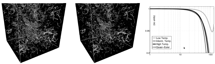
Figure 1 shows the local superfluid and normal fluid enstrophies $|{\mbox{\boldmath$\omega_{s}$}}|^{2}$ (left) and $|{\mbox{\boldmath$\omega_{n}$}}|^{2}$ (right) at the intermediate temperature ($\rho_{n}=\rho_{s}$). Intense vortex regions (“worms”) are highlighted by the colour scale, which becomes gray above $5<|{\mbox{\boldmath$\omega_{s}$}}|^{2}>$ and opaque white above $10<|{\mbox{\boldmath$\omega_{s}$}}|^{2}>$, where the symbol $<\cdots>$ indicates volume averaging . The figure clearly shows that the vorticity structures of the two fluids are very similar. The degree of similarity can be quantified by the correlation coefficient

$$c_{1}=\frac{<{\mbox{\boldmath$\omega_{s}$}}{\mbox{\boldmath$\omega_{n}$}}>}{\sqrt{<{\mbox{\boldmath$\omega_{s}$}}^{2}><{\mbox{\boldmath$\omega_{n}$}}^{2}>}},$$ (4)

We find that $c_{1}$ is larger than $97\%$ at all three temperatures explored, in agreement with recent numerical calculations [23] of a superfluid vortex tangle driven by a turbulent normal fluid at high temperature ($\rho_{n}/\rho_{s}\simeq 3$). Unlike our work, these simulations ignored the back–reaction of the vortex tangle onto the normal fluid.

The plot on the right side of Fig. 1 compares the spectral coherence function

$$c_{2}(k)=\frac{|\mathbf{v}_{n}(k).\overline{\mathbf{v}_{s}(k)}|^{2}}{|\mathbf{v}_{n}(k)|^{2}.|\mathbf{v}_{s}(k)|^{2}}$$ (5)

of superfluid and normal fluid velocity fields: The fact that $c_{2}(k)$ is larger than 98% at all scales below $k_{max}/4$, where $k_{max}=128$ is the largest wave vector associated with our 256³ mesh, means that superfluid and normal fluid velocity fields are strongly locked along the inertial range, up to the forcing length scale, where the energy, which is injected into one fluid only, is redistributed very efficiently over both fluids. We recall that energy is injected into the normal fluid only, except at low temperature, where it is injected in the superfluid only.

Figure 2: [colour online] Subplot a : Spectra of the magnitude of the superfluid vorticity $|{\mbox{\boldmath$\omega_{s}$}}|$ vs wavenumber $k$. From top to bottom low [green], intermediate [blue] and high [red] temperatures. Subplot b / Upper part: Superfluid (thick solid lines) and normal fluid (thick dashed lines) velocity power spectra vs wavenumber $k$ at the three temperatures. The thin dashed line denotes the Kolmogorov $k^{-5/3}$ scaling. Subplot b / Lower part: The thin solid lines show the spectra of the slip velocity at the three temperatures.

The upper set of curves of Fig. 2b presents the superfluid and normal velocity power spectra $E_{n}(k)$ and $E_{s}(k)$ (defined by $E_{i}=\int E_{i}(k)dk$ ($i=n,s)$ where $E_{i}$ is the total energy in arbitrary units) at high, intermediate and low temperature. As expected from the previous figure, the spectra overlap along the inertial range; around $k=10$, both spectra are compatible with Kolmogorov’s $k^{-5/3}$ inertial range scaling (illustrated by the thin straight line). Note also that at each temperature, since $\nu_{s}<\nu_{n}$, for increasing $k$ the normal fluid becomes damped before the superfluid. This is consistent with Fig. 1, which shows that the superfluid enstrophy is indeed stronger than the normal fluid’s.

3.2 The slip between the two fluids

If the two fluids were perfectly locked, the mutual friction would be zero, which would inevitably result in the unlocking of the two fluids, as they would experience different forcing and dissipation processes. A residual slip velocity $\mathbf{v}_{ns}=\mathbf{v}_{s}-\mathbf{v}_{n}$ between the two fluid must therefore be present. The lower set of curves in Fig.2b shows the spectrum of $\mathbf{v}_{ns}$. The peak at $k\approx 2$ is caused by the forcing, which is applied to a single fluid, and induces a residual slip at this wavevector. The striking feature of this spectrum is that it increases with $k$ in the inertial range, starting at $k\sim 10$, and peaking in the dissipation scales, where the dissipation of one fluid is significantly larger than that of the other. The increase with $k$ of the slip velocity spectrum is remarkably pronounced in the “quasi-Euler” case.

3.3 Energy transfer between the two fluids

We focus on the high temperature “quasi-Euler” case ($\nu_{n}/\nu_{s}=100$, $\rho_{n}/\rho_{s}=10$) because it is expected to mimic He II hydrodynamics more closely than other viscosity ratios. The scale–by–scale energy budget per mass unit for the normal fluid and superfluid are respectively:

$$\frac{\partial E_{n}}{\partial t}(k,t)=-D_{n}(k,t)-T_{n}(k,t)-M_{n\to s}+\epsilon^{inj}\delta_{k,2},$$ (6)

$$\frac{\partial E_{s}}{\partial t}(k,t)=-D_{s}(k,t)-T_{s}(k,t)-M_{s\to n},$$ (7)

where $D_{n}$ and $D_{s}$ are the viscous dissipation terms in the normal fluid and superfluid,

$$D_{i}(k,t)=2\nu_{i}k^{2}E_{i}(k,t)$$ (8)

$T_{n}$ and $T_{s}$ are the energy transfer rates arising from triad interactions between Fourier modes within each fluid; the energy flux at wave number k related to the non-linear interaction is defined by

$$F_{i}(k,t)=\int_{0}^{k}T_{i}(k^{\prime},t)dk^{\prime}.$$ (9)

$M_{s\to n}$ and $M_{n\to s}$ result from the exchange of kinetic energy between the two fluids by mutual friction :

$$M_{n\to s}(k,t)=-\frac{\rho_{s}}{\rho}(\mathbf{F}_{ns}\cdot\mathbf{v}_{n})(k,t),$$ (10)

$$M_{s\to n}(k,t)=\frac{\rho_{n}}{\rho}(\mathbf{F}_{ns}\cdot\mathbf{v}_{s})(k,t).$$ (11)

Figure 3: [colour online] Energy exchange between fluids in the high temperature “quasi-Euler” case ( $\rho_{n}/\rho_{s}=10$ and $\nu_{n}/\nu_{s}=100$).

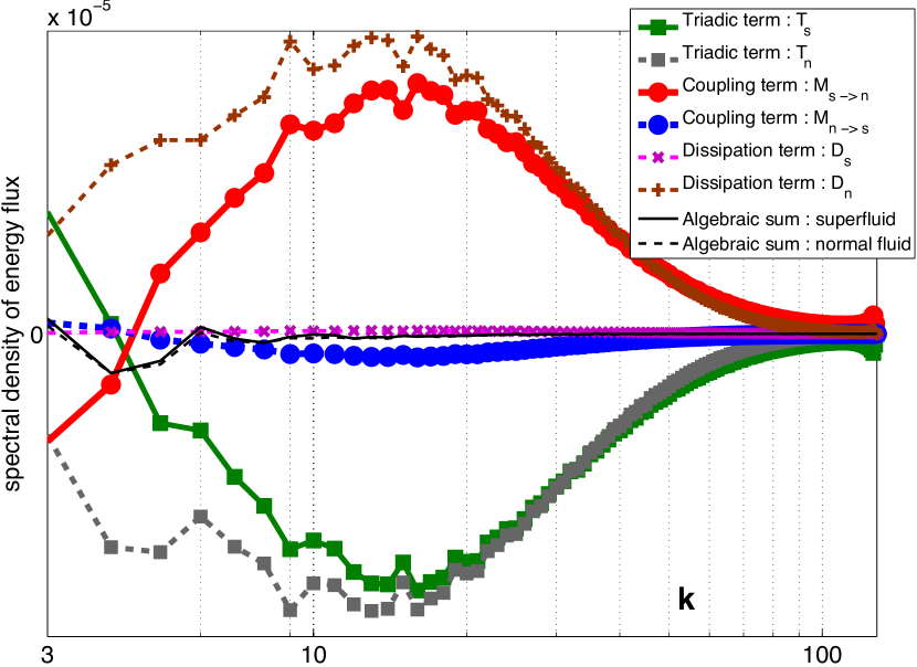
Dissipations, triadic interactions and mutual coupling terms in $k$ space are shown in Figure 3. As expected from the stationary of the flow, for each fluid the sum of all terms is close to zero, except at the lowest $k$ (for which volume averaging is not performed over enough independent realisations due to the limited time scale of integration). In the inertial range and in the near dissipative range, the triadic interaction terms for both fluids are the same at first order, as expected from $\mathbf{v}_{n}\simeq\mathbf{v}_{s}$. In the normal fluid, the triadic term is roughly compensated by the viscous dissipation. In the superfluid, the viscous dissipation is $\nu_{n}/\nu_{s}=100$ times smaller, and the triadic term is compensated instead by the coupling term. For consistency, we check that this coupling has a second order effect on the normal flux budget: we find $|M_{n\to s}/M_{s\to n}|\simeq\rho_{s}/\rho_{n}=0.1$. We conclude that in the inertial range at high temperatures: the slip velocity allows energy to leak from the superfluid with a flux which mimics the normal fluid viscous dissipation, so that both fluid end up with similar behaviour. This process remains compatible with a strong locking of the 2 fluids in the limit of high Reynolds numbers.

3.4 The dissipation cut–off in the two–fluids cascade

In ordinary Navier-Stokes homogeneous turbulence, the viscous cut–off scale $\eta$ is determined by the energy injection $\epsilon$ at large scale $d_{0}$ and by the kinematic viscosity $\nu$:

$$\eta^{4}\approx\frac{\nu^{3}}{\epsilon}.$$ (12)

With the exception of the “quasi-Euler” case, the spectra of $\mathbf{v}_{n}$ and $\mathbf{v}_{s}$ are computed with the same viscosities $\nu_{n}$ and $\nu_{s}$ and the same total energy injected per unit volume at wavenumber $k\simeq 2$. The collapse of all spectra onto the same curve at low $k$ shown in Fig. 2b indicates that the energy injected is efficiently redistributed between the two fluids, and that both fluids have the same integral scale $d_{0}$ (as evident in Fig.1). Contrary to what happens in single–fluid Navier-Stokes turbulence, Fig. 2b shows that the superfluid and normal fluid cutoff–scales are temperature dependent: it is apparent that the lower is $T$, the more extended is the inertial range cascade. Therefore, if one defines the Reynolds number using the classical relation with the ratio of large and small scales of the cascade, $Re=(\eta/d_{0})^{-4/3}$, one finds that $Re$ is temperature dependent. Evidently, ordinary turbulent relations such as Eq.12 are not valid in our two–fluids system.

We now argue that the temperature dependence of $\eta$ and $Re$ observed for finite $\nu_{s}$ will be present in the limit $\nu_{s}=0$, and will reflect the temperature-dependent efficiency of the energy transfer from the superfluid to the normal by mutual friction. This process is independent of $\nu_{n}$, and more generally is independent of the dissipation mechanism in the normal fluid. It can be accounted by a temperature-dependent effective superfluid viscosity $\nu_{eff}$.

As a starting point, we note in Fig. 2b that at small enough scales $|\mathbf{v}_{n}|<<|\mathbf{v}_{s}|$. At these small scales the mutual friction force in the equation for $\mathbf{v}_{s}$ simplifies to

$$-\frac{\rho_{n}}{\rho}\mathbf{F}_{ns}=-\frac{\rho_{n}}{\rho}\frac{B}{2}|{\mbox{\boldmath$\omega_{s}$}}|(\mathbf{v}_{n}-\mathbf{v}_{s})\approx\alpha|{\mbox{\boldmath$\omega_{s}$}}|\mathbf{v}_{s},$$ (13)

where $\alpha=\rho_{n}B/(2\rho)$[18]. In our model, the prefactor $|{\mbox{\boldmath$\omega_{s}$}}|$ in the mutual friction accounts for the local absolute vorticity of the vortex tangle, which, following Ref. [9], can be related to the vortex line density by $|{\mbox{\boldmath$\omega_{s}$}}|=\kappa L$. If the vortex lines are smooth on length scales of order $\ell\approx L^{-1/2}$, the quantity $\ell$ measures the inter-vortex spacing and corresponds to the cut-off scale of superfluid turbulence. We conclude that at sufficiently small scales

$$-\frac{\rho_{n}}{\rho}\mathbf{F}_{ns}\approx\alpha\kappa L\mathbf{v}_{s}\approx\nu_{eff}(\frac{\mathbf{v}_{s}}{\ell^{2}}).$$ (14)

where the analogy between ${\mathbf{v}_{s}}/{\ell^{2}}$ and the magnitude of $\nabla^{2}\mathbf{v}_{s}$ has suggested the introduction of an effective superfluid viscosity:

$$\nu_{eff}=\alpha\kappa,$$ (15)

This effective viscosity is relevant at scales smaller or equal to $l$, at which superfluid energy is transferred into the normal fluid by mutual friction.

When comparing our DNS model to experiments we must remember that in our continuous model the identification $L=|{\mbox{\boldmath$\omega_{s}$}}|/\kappa$ neglects random vortex filaments and Kelvin waves of wavelength shorter than $\ell$ (which become particularly important at very low temperatures), thus underestimating the vortex line density. It is therefore more proper to relate $\ell$ not to the total $L^{-1/2}$ but to $L_{\parallel}^{-1/2}$, defined in our previous paper [16] as the vortex line density associated with the polarised part of the vortex tangle. Eq. 15 thus becomes

$$\nu_{eff}=\frac{L}{L_{\parallel}}\alpha\kappa$$ (16)

where the ratio $L/L_{\parallel}\geqslant 1$ is expected to be of order one at high temperature and possibly significantly larger than one in the limit $T\to 0$. This ratio measures the wiggleness of the tangle at small scale, and can be interpreted as a measure of its fractal dimension[26].

Figure 4: [Colours online]. Effective kinematic viscosity in units of $\kappa$. Isolated symbols: Superfluid effective viscosity defined by $\nu_{eff}^{\prime}=\epsilon/(\kappa L)^{2}$ and measured in decaying turbulence experiments; [blue] diamonds [5], [red] circles [27], [green] squares [8] and triangles [28, 29]. Lines: analytical models; thick [black] line: present model (Eq.16) with prefactor $L/L_{\parallel}=2$ ( isolated bullet [black] for $L/L_{\parallel}=30$), thin [purple] continuous line: $\mu/(\rho\kappa)$ where $\mu$ is the dynamic viscosity of the normal fluid; dashed [grey] lines: microscopic model Eq. 66 from Ref. [9] computed with prefactor $R_{0}/a_{0}=10^{6}$ and $10^{4}$

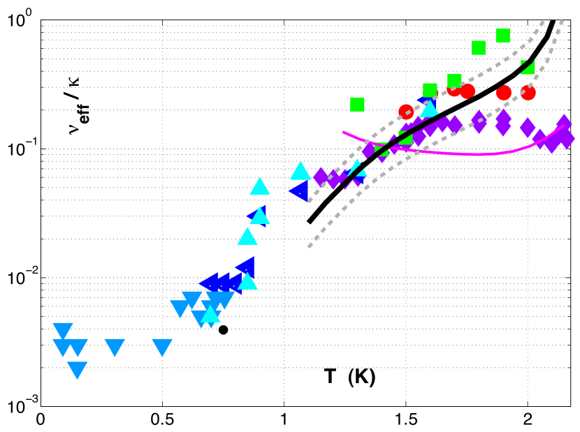
An alternative derivation of an effective superfluid viscosity has been proposed in Ref. [9] (page 216) from the more microscopic point of view of the friction of individual vortex lines. Fig.4 shows that our macroscopic model of $\nu_{eff}$ (thick black line) is in excellent agreement with the microscopic model of Ref. [9](thin grey dashed lines). In the figure our model is plotted with a wiggleness prefactor $L/L_{\parallel}=2$, and the model of Ref. [9] contains a logarithmic prefactor which has been estimated for two different sets of parameters for laboratory turbulent flows.

Another (experimental) definition of effective superfluid viscosity $\nu_{eff}^{\prime}=\epsilon/(\kappa L)^{2}$ has been proposed in recent studies of decaying turbulence experiments [5, 27, 8, 28, 29]. These values of $\nu_{eff}^{\prime}$ are shown in Fig.4 as symbols. The agreement between $\nu_{eff}$ and $\nu_{eff}^{\prime}$ is good. Since $B$ is approximately constant with temperature above 1K, the strong temperature dependent of the effective viscosity arises from the temperature dependence of $\rho_{n}/\rho$, which suggests that the ratio $L/L_{\parallel}$ has little temperature dependence above 1K.

Although what happens below $1~{}K$ goes beyond the scope of this study, we remark that there is a qualitative good agreement between experimental data below 1K and the low temperature extrapolation of the predicted effective viscosity. A wiggliness prefactor $L/L_{\parallel}\simeq 30$ would allow to account for the measured effective viscosity down to 750 mK typically. This suggests that the cross-over between zero-temperature and finite temperature quantum turbulence occurs at a lower temperature than the usual estimation of $1~{}\rm K$ based on phonon (normal fluid) mean free path considerations. In other words, it suggests that a relative small concentration of normal fluid (significantly lower than 1 percent) still produces a dissipation which is comparable to other effects (Kelvin waves cascade, vortex reconnections) which are specific of the superfluid. Although our continuous model is no longer justified for the normal fluid below $1~{}\rm K$, this observation is not inconsistent with it, because $\nu_{eff}$ is derived regardless of the normal fluid dynamics.

Finally, we speculate on the form of the classical Eq.12 for superfluids. Following the analogy between the mutual friction at small scale and the viscous dissipation (Eq.14), the kinetic energy which is “removed” from the superfluid at small scales is

$$\epsilon\approx\nu_{eff}(\frac{v_{s}^{2}}{\ell^{2}}).$$ (17)

Substituting $v_{s}\approx\kappa/\ell$. into Eq.17, we recognise the alternative definition $\nu_{eff}^{\prime}$. Combining Eq.17 and Eq.16, we obtain the following superfluid counterpart of the classical Eq.12:

$$\ell^{4}=(\frac{\rho_{n}}{\rho}\frac{B}{2})\frac{\kappa^{3}}{\epsilon}\frac{L}{L_{\parallel}}=\frac{\alpha\kappa^{3}}{\epsilon}\frac{L}{L_{\parallel}},$$ (18)

where the wiggleness parameter $L/L_{\parallel}$ is of order one for $T>1$ K and possibly larger at lower temperatures. Note that Eq. 18 contains an implicit temperature dependence through $B$ and ${\rho_{n}}/{\rho}$ (and possibly through $L/L_{\parallel}$ in the low temperature limit).

A quantitative comparison of Eq. 18 with our numerical simulations is impossible due to the finiteness of $\nu_{s}$ in particular, but we find a good qualitative agreement. Eq. 18 allows us to predict the temperature dependence of the depth of the turbulent cascade, and to define a ”superfluid Reynolds number” using the separation of large and small scales.

4 Conclusion and Perspectives

We have introduced a new two–fluids DNS model to study quantum turbulence in a self–consistent way. The model is based on the continuum approximation, and we have discussed its advantages and limitations. Our numerical results support the current understanding [9] that in quantum turbulence the superfluid and the normal fluid are strongly coupled. In addition, our results at high temperature show the slip velocity peaks in the dissipation scales, and that whereas in the normal fluid the triadic interaction is balanced by the viscous dissipation, in the superfluid it is balanced by the mutual friction. We have also found that the usual turbulence relation (Eq.12) which relates the cutoff scale to the energy injection at large scale $\epsilon$ and the kinematic viscosity $\nu$ is not valid in our two–fluids system. Finally, we have found that the energy transfer from the superfluid to the normal fluid does not depend on the normal fluid’s dissipation, but it can be accounted by a temperature–dependent effective superfluid viscosity $\nu_{eff}$, which we have calculated and which is in good agreement with other estimates. Using this quantity, we have obtained the superfluid equivalent (Eq. 18) to the classical formula (Eq. 12) which relates the energy injection to the dissipation scale.

In discussing our result we have introduced the wiggleness parameter $L/L_{\parallel}$ which is or order one above $1~{}\rm K$ but may be larger at smaller temperatures. We speculate that $L/L_{\parallel}$ is related to the fractal dimension of the tangle; its increase in the low temperature limit may explain the saturation of $\nu_{eff}$ for $T\to 0$. Further work will solve this issue.

In two recent experiments [6, 30], the spectrum of vortex line density in turbulent superfluids was found to differ from its classical counterpart: the spectrum of local enstrophy. A proposed interpretation assumes that only the “polarised” contribution of the vortex tangle mimics the classical enstrophy [16]. The present numerical model, which only accounts for the polarised contribution, gives results consistent with this picture : the spectrum of the superfluid vorticity $|{\mbox{\boldmath$\omega_{s}$}}|$ (Fig. 2a) is indeed similar to corresponding spectra in classical fluids.

Future work will also attempt to test further the proposed interpretation[16] by adding to the current DNS two–fluids model an equation for a scalar field field accounting for the density of the unpolarised contribution of the vortex tangle. Another important problem to address is the decay of turbulence, which is receiving much experimental attention.