Programming Realization of Symbolic Computations for Non-linear Commutator Superalgebras over the Heisenberg–Weyl Superalgebra: Data Structures and Processing Methods

Abstract

We suggest a programming realization of an algorithm for a verification of a given set of algebraic relations in the form of a supercommutator multiplication table for the Verma module, which is constructed according to a generalized Cartan procedure for a quadratic superalgebra and whose elements are realized as a formal power series with respect to non-commuting elements. To this end, we propose an algebraic procedure of Verma module construction and its realization in terms of non-commuting creation and annihilation operators of a given Heisenberg–Weyl superalgebra. In doing so, we set up a problem which naturally arises within a Lagrangian description of higher-spin fields in anti-de-Sitter (AdS) spaces: to verify the fact that the resulting Verma module elements obey the given commutator multiplication for the original non-linear superalgebra. The problem setting is based on a restricted principle of mathematical induction, in powers of inverse squared radius of the AdS-space. For a construction of an algorithm resolving this problem, we use a two-level data model within the object-oriented approach, which is realized on a basis of the programming language C#. The first level, the so-called basic model of superalgebra, describes a set of operations to be realized as symbolic computations for arbitrary finite-dimensional associative superalgebras. The second level serves to realize a specific representation of non-linear commutator superalgebra elements, and specifies the peculiarities of commutation operations for the elements of a specific superalgebra $\mathcal{A}$, as well as the ordering of creation $f^{+},b_{i}^{+}$ and annihilation $f,b_{i}$, $i=1,2$, operators in products which determine supercommutators $[a,b\}$, $a,b\in\mathcal{A}$, to be verified. The program allows one to consider objects (of a less general nature than non-linear commutator superalgebras) that fall under the class of so-called $GR$-algebras, for whose treatment one widely uses the module Plural of the system Singular of symbolic computations for polynomials.

Keywords: nonlinear operator superalgebra, $G$-algebra, Verma module, symbolic computation, data structures, C#

AMS subject classifications. 68W30, 16S37, 17B10, 16S99, 17-08

1 Introduction

The problem of treatment of algebraic structures more general than Lie algebras [1] and superalgebras [2], equivalent, in fact, to matrix algebras and superalgebras, is a relatively recent issue in the area of Theoretical Physics and Pure and Applied Mathematics; for a review of notions on non-linear algebras, see the textbook [3]. Mathematically, this trend gains its motivation from the study of nonlinear algebras and superalgebras, such as $W$-algebras [4], whereas from the physical viewpoint it is due to an intensive application of nonlinear algebraic structures in High Energy Physics, in particular, within the theory of strings and superstrings [5] and the related Higher Spin Field Theory; for a review see [6]. Field-theoretical models of higher-spin (HS) fields in constant-curvature spaces (Minkowski, de Sitter, anti-de-Sitter) related to the hope of detection (perhaps in view of the expected launch of LHC), at a level of energy higher than the level presently accessible to physical laboratories, of new kinds of interactions and particles which must be part of superstring spectrum. It should be noted that the choice of the anti-de-Sitter (AdS) space presents, first of all, the simplest non-trivial background providing a consistent propagation of free [7] and interacting HS fields, since the radius of the AdS space ensures the presence of a natural dimensional parameter for an accommodation of compatible self-interactions [8, 9]. Second, the (A)dS space is the most adequate model for a description of space-time corresponding to the Universe, in view of the modern data [10] on its accelerated expansion. Third, HS fields in the AdS space are closely related to the tensionless limit of superstring theory on the $AdS_{5}\times S_{5}$ Ramond–Ramond background [11, 12] and the conformal $\mathcal{N}=4$ SYM theory in the context of the AdS/CFT correspondence [13].

For a quantum description of an HS field in the AdS_d-spaces within conventional Quantum Field Theory, it is necessary to construct its gauge-invariant Lagrangian description, which includes a determination of the action functional and of the set of reducible gauge symmetries [14, 15]; for the pioneering works on this problem, see for instance [16]. Among different methods which allow one to solve this problem, an especially outstanding one is the BFV–BRST approach, inspired by Witten’s String Field Theory [5], and based on a special global BRST symmetry [25] and on the BFV method [26], realizing this symmetry within the Hamiltonian description of dynamical systems with constraints.

For the purpose of this work, it is appropriate to mention that the central object of the BFV–BRST approach, the BFV–BRST operator, is constructed, in the case of the AdS_d-space, with respect to a non-linear (super)algebra $\mathcal{A}_{c}(Y(1),AdS_{d})$, $\mathcal{A}_{c}(Y(1),AdS_{d})$ =$\mathcal{A}(Y(1),AdS_{d})$ + $\mathcal{A}^{\prime}(Y(1),AdS_{d})$, for a (half-)integer spin ($s=n+\frac{1}{2}$, $n\in\mathbb{N}_{0}$) $s,s\in\mathbb{N}_{0}$ subject to a Young tableaux with one row. The operators $O_{I}$, $O_{I}=(o_{I}+o^{\prime}_{I})$, composing this (super)algebra $O_{I}\in\mathcal{A}_{c}(Y(1),AdS_{d})$ are determined in a special Hilbert space $\mathcal{H}_{c}$, $\mathcal{H}_{c}=\mathcal{H}\otimes\mathcal{H}^{\prime}$, with respect to differential algebraic relations which extract a field (tensor, $s\in\mathbb{N}_{0}$, or spin-tensor, $s=n+\frac{1}{2}$) of given mass $m$ and spin $s$ from the space of unitary irreducible representation of the AdS group in the AdS_d space.

Having restricted this paper by the case of a half-integer spin, we note that the deduction of the superalgebra $\mathcal{A}_{c}(Y(1),AdS_{d})$ is based [27] on the construction of an auxiliary representation, called the Verma module [33], for a quadratic superalgebra $\mathcal{A}^{\prime}(Y(1),AdS_{d})$, coinciding with the superalgebra $\mathcal{A}(Y(1),AdS_{d})$ in a flat space, $r=0$, i.e., for the Lie superalgebra $\mathcal{A}(Y(1),\mathbb{R}^{d-1,1})$. The Verma module provides a correct number of physical degrees of freedom in a non-Abelian conversion method [34] and therefore ensures an application of the BFV–BRST approach. While the problem of Verma module construction is solved for Lie algebras [35] and superalgebras [36, 37], for the quadratic [38] operator algebra $\mathcal{A}_{b}(Y(1),AdS_{d})$ used in Ref. [39] to construct a Lagrangian formulation for bosonic HS fields in the AdS_d-space subject to $Y(1)$, the corresponding problem for the non-linear superalgebra $\mathcal{A}^{\prime}(Y(1),AdS_{d})$ is yet unsolved, leaving the correctness of the Lagrangian formulation of Ref. [27] questionable.

The principal goals of this paper are as follows:

1. development of a method of constructing the Verma module $V_{\mathcal{A}^{\prime}}$ for a non-linear superalgebra $\mathcal{A}^{\prime}(Y(1),AdS_{d})$ on the basis of a generalized Cartan procedure;

2. realization of the Verma module $V_{\mathcal{A}^{\prime}}$ in terms of a formal power series in the degrees of non-supercommuting generating elements $b_{i},b_{i}^{+},f,f^{+},i=1,2$ of the Heisenberg–Weyl superalgebra, whose number coincides with those of negative $\{E^{-A}\}$ and positive $\{E^{A}\}$ root vectors in a Cartan-like decomposition $\mathcal{A}^{\prime}(Y(1),AdS_{d})$ = $\mathcal{E}^{-A}\oplus\mathcal{H}^{\hat{i}}\oplus\mathcal{E}^{A}$ (with Cartan subsuperalgebra $\mathcal{H}^{\hat{i}}$).

In connection with a solution of these problems, there arises a number of peculiarities, stipulated by the fact that the elements of the Verma module $V_{\mathcal{A}^{\prime}}$ are constructed with respect to a given multiplication for the superalgebra $\mathcal{A}^{\prime}(Y(1),AdS_{d})$ in an indirect way:

• first, the Verma module $V_{\mathcal{A}^{\prime}}$ is derived by means of the Cartan procedure, and then it is realized as a formal power series $o^{\prime}_{I}(b_{i},b_{i}^{+},f,f^{+})$; as a consequence, one needs a formal proof of the fact that these operators $o^{\prime}_{I}(b_{i},b_{i}^{+},f,f^{+})$ actually satisfy the table of supercommutator multiplication for $\mathcal{A}^{\prime}(Y(1),AdS_{d})$;

• in view of a sufficiently large number of basis elements, $l=9$, for $\mathcal{A}^{\prime}$, which grows with the increasing of the rows of the Young tableaux, so that for $\mathcal{A}^{\prime}(Y(k),AdS_{d})$ the number of basis elements is equal to $2(1+k^{2}+\frac{5}{2}k)$, from the technical viewpoint the problem of verifying the given algebraic relations is quite time-consuming.

Therefore, the next group of problems to be solved in this paper is the following:

1. finding a formalized setting of the problem of verifying the fact that the operators $o^{\prime}_{I}(b_{i},b_{i}^{+}$, $f,f^{+})$ obey the given algebraic relations $\mathcal{A}^{\prime}(Y(1),AdS_{d})$ with the help of a restricted induction principle, in powers of the inverse squared radius $r$ of the AdS_d-space;

2. realization, in a high-level programming language ($C\#$), of an algorithm of solving the above problem by using the techniques of symbolic calculations.

From the viewpoint of mathematics and programming, the problem of symbolic computations (the symbols here are the elements of the Heisenberg–Weyl superalgebra $b_{i},b_{i}^{+},f,f^{+}$ and polynomials constructed from them) with respect to non-linear superalgebras has not been considered, and, to our knowledge (see, for instance, [40] and references therein), has not been realized as a computer program. The particular case of the flat space $\mathbb{R}^{1,d-1}$ for $r=0$ is an exception where such well-known application packages as Maple, MathLab, MathCad, Mathematica, etc., permit one to operate with the Lie superalgebra $\mathcal{A}^{\prime}(Y(1),\mathbb{R}^{1,d-1})$, equivalent to supermatrix algebras. In addition, formal power series $o^{\prime}_{I}(b_{i},b_{i}^{+},f,f^{+})$ pass in this case to finite-order polynomials of at most third degree with respect to $b_{i},b_{i}^{+},f,f^{+}$, so that the solution of problem $3$ appears quite trivial for a calculator. It should be noted that among the programs being the most capable to work with symbolic calculations one widely uses the module Plural [41] of the system Singular for symbolic calculations of polynomials, which is intended for computations in a class of non-commuting polynomial algebras. Left ideals and modules over a given non-commutative $G$-algebra [42], so-called, $GR$-algebras, are the basic objects of calculations using Plural. At the same time, the case of the nonlinear superalgebra $\mathcal{A}^{\prime}(Y(1),AdS_{d})$ under consideration has a number of supercommutator relations that cannot be realized within the class of $G$-algebras and therefore in Plural as well.

The paper is organized as follows. In Section 2, we introduce necessary algebraic definitions, examine a special nonlinear operator superalgebra $\mathcal{A}^{\prime}(Y(1),AdS_{d})$, whose algebraic relations were obtained in Ref. [27], explicitly construct the Verma module $V_{\mathcal{A}^{\prime}}$, find a realization of $V_{\mathcal{A}^{\prime}}$ in terms of a formal power series in noncommuting elements (symbols) of the Heisenberg–Weyl superalgebra $A_{1,2}$, and set up a formalized representation for $\mathcal{A}^{\prime}(Y(1),AdS_{d})$. In Section 3, we consider in detail the elements of a programming realization using $C\#$ to solve the formalized setting of the problem on the basis of a two-level model for a representation of the Verma module for a nonlinear superalgebra, which includes a so-called basic model of superalgebra and model of polynomial superalgebra. We apply the developed program to a verification of the required algebraic relations for the superalgebra $\mathcal{A}^{\prime}(Y(1),AdS_{d})$ in Section 4. In Section 5, we summarize the results of the paper and discuss the perspectives of applying the program.

2 Non-Linear Superalgebras

In this section, we introduce the definitions of a non-linear superalgebra with respect to commutator multiplication and study a number of its algebraic properties for a solution of the basic algebraic problems for a special operator superalgebra. We then use our construction to develop a problem setting in order to fulfill a program verification of the fact that a given oscillator realization of the above superalgebra actually satisfies a given multiplication table.

2.1 Basic definitions and algebraic constructions

Let $\mathbb{K}$ be a field and $\mathcal{A}=\{e,o_{I}\}$, $I\in\Delta$ be an associative $\mathbb{K}$-superalgebra with unity $e$ and a basis $\{e,o_{I}\}$, being a two-side module over a Grassmann algebra $\Lambda=\{\alpha_{k}\}$, $k\in X$, where $\Delta$ and $X$ are independent finite or infinite sets of indices.

Definition 1. Associative $\mathbb{K}$-superalgebra $\mathcal{A}$ over $\Lambda$ is called a non-linear Lie-type superalgebra if there exists a two-place operation $[\ ,\ \}$ satisfying the following conditions for $I,J,K\in\Delta$, $k,l\in X$:

$$\mathbf{-Non-linearity} [o_{I},o_{J}\}=F^{K}_{IJ}(o)o_{K},\ F^{K}_{IJ}=f^{(1)K}_{IJ}+\sum_{n=2}^{\infty}f^{(n)K_{1}...K_{n-1}K}_{IJ}\prod_{i=1}^{n-1}o_{K_{i}};$$ (1)

$$\mathbf{-Antisymmetry\ } [o_{I},o_{J}\}=-(-1)^{\varepsilon_{I}\varepsilon_{J}}[o_{J},o_{I}\};$$ (2)

$$\mathbf{-\Lambda-bilinearity\ } [\alpha_{k}o_{I}+\alpha_{l}o_{J},o_{K}\}=\alpha_{k}[o_{I},o_{K}\}+\alpha_{l}[o_{J},o_{K}\},$$

$$[o_{I},\alpha_{k}o_{J}+\alpha_{l}o_{K}\}=(-1)^{\varepsilon_{I}\varepsilon_{k}}\alpha_{k}[o_{I},o_{J}\}+(-1)^{\varepsilon_{I}\varepsilon_{l}}\alpha_{l}[o_{I},o_{K}\};$$ (3)

$$\mathbf{-Leibnitz\ rule\ \ \ } [o_{I},o_{J}o_{K}\}=[o_{I},o_{J}\}o_{K}+(-1)^{\varepsilon_{I}\varepsilon_{J}}o_{J}[o_{I},o_{K}\}$$ (4)

$$\mathbf{-Jacobi\ identity} (-1)^{\varepsilon_{I}\varepsilon_{K}}[o_{I},[o_{J},o_{K}\}\}+cycl.perm.(I,J,K)=0,$$ (5)

where we suppose summation with respect to repeated indices $K_{1},...,K_{n-1},K$ in (1); the quantities $f^{(1)K}_{IJ},f^{(n)K_{1}...K_{n-1}K}_{IJ}\in\Lambda$ obey the antisymmetry properties

$$\bigl{(}F^{K}_{IJ}(o),f^{(1)K}_{IJ},f^{(n)K_{1}...K_{n-1}K}_{IJ}\bigr{)}=-(-1)^{\varepsilon_{I}\varepsilon_{J}}\bigl{(}F^{K}_{JI}(o),f^{(1)K}_{JI},f^{(n)K_{1}...K_{n-1}K}_{JI}\bigr{)},$$ (6)

and $\varepsilon_{I},\varepsilon_{k}$ are the Grassmann parities of the elements $o_{I}$, $\alpha_{k}$, $(\varepsilon_{I},\varepsilon_{k})$ $\equiv$ $(\varepsilon(o_{I}),\varepsilon(\alpha_{k}))$, being equal respectively to 0 and 1 for even and odd $o_{I},\alpha_{k}$ with respect to a given $\mathbb{Z}_{2}$-grading in $\mathcal{A}$.

It should be noted, first, that the property (4) presents the compatibility of the associative and Lie-type multiplications in $\mathcal{A}$. Second, a typical example of a non-linear Lie-type superalgebra is the classical analogue of finite-dimensional non-linear superalgebras [43] where the operation $[\ ,\ \}$ is the Poisson superbracket $\{\ ,\ \}$.

Definition 2. A non-linear Lie-type superalgebra $\mathcal{A}$ is called a non-linear commutator superalgebra if the two-place operation $[\ ,\ \}$ is realized as a supercommutator for any $A,B\in\mathcal{A}$ with definite Grassmann gradings $\varepsilon(A),\varepsilon(B)$

$$[A,B\}=AB-(-1)^{\varepsilon(A)\varepsilon(B)}BA.$$ (7)

Definition 3. A non-linear commutator (Lie-type) superalgebra $\mathcal{A}$ is called a polynomial (Lie type) superalgebra of order $n$, $n\in\mathbb{N}$, if decomposition (1) obeys the following condition:

$$f^{(n)KK_{1}...K_{n}}_{IJ}\neq 0,\ and\ f^{(k)KK_{1}...K_{n}K_{n+1}...K_{k}}_{IJ}=0,\ k>n,k\in\mathbb{N}.$$ (8)

Corollary 1. Polynomial superalgebras of order $1$, $2$ correspond to Lie superalgebras [2] and quadratic superalgebras [27], such as superconformal algebras, extending the case of quadratic algebras [44, 4].

It should be noted that within the class of polynomial algebras and superalgebras of definite order $k$ there exist superalgebras [28], [29] with so called parasupersymmetry and superalgebras with only parabosonic elements [30], the ones with non-linear realization of the supersymmetry used in the framework of mechanics, in description of Aharonov-Bohm effect [31], [32].

It is interesting to observe the structure of the following relations for a non-linear Lie type superalgebra, starting from the resolution of the Jacobi identity (5) for the elements $\{o_{I}\}$. In doing so, we may follow two ways: first, a purely algebraic approach, and, second, a more general gauge-inspired approach [26, 45]. For instance, in the case of a supercommutative quadratic Lie-type superalgebra (which can be considered as a generalization of a so-called Poisson $L-T$ algebra [46] to the case of a superalgebra, if $[\ ,\ \}$ is a Poisson bracket realized in a corresponding phase space), we may obtain two sets of relations which present a solution of the Jacobi identity (5):

$$\Bigl{\{}(-1)^{\varepsilon_{I}\varepsilon_{K}}\Bigl{[}f^{(1)K_{1}}_{IJ}f^{(1)L_{3}}_{K_{1}K}+\bigl{(}f^{(1)K_{1}}_{IJ}f^{(2)L_{2}L_{3}}_{K_{1}K}+(-1)^{\varepsilon_{K}\varepsilon_{L_{3}}}f^{(2)K_{1}L_{3}}_{IJ}f^{(1)L_{2}}_{K_{1}K}$$

$$+(-1)^{\varepsilon_{L_{2}}(\varepsilon_{L_{3}}+\varepsilon_{K_{1}}+\varepsilon_{K})}f^{(2)L_{2}K_{1}}_{IJ}f^{(1)L_{3}}_{K_{1}K}\bigr{)}o_{L_{2}}+\bigl{(}(-1)^{\varepsilon_{K}\varepsilon_{L_{3}}}f^{(2)K_{1}L_{3}}_{IJ}f^{(2)L_{1}L_{2}}_{K_{1}K}$$

$$+(-1)^{\varepsilon_{L_{1}}(\varepsilon_{L_{2}}+\varepsilon_{L_{3}}+\varepsilon_{K_{1}}+\varepsilon_{K})}f^{(2)L_{1}K_{1}}_{IJ}f^{(2)L_{2}L_{3}}_{K_{1}K}\bigr{)}o_{L_{1}}o_{L_{2}}\Bigr{]}+cycl.perm.(I,J,K)\Bigr{\}}o_{L_{3}}=0,$$ (9)

in the algebraic approach, with the use of the obvious symmetry property for $f^{(2)K_{1}K_{2}}_{IJ}$, $f^{(2)K_{1}K_{2}}_{IJ}=(-1)^{\varepsilon_{K_{1}}\varepsilon_{K_{2}}}f^{(2)K_{2}K_{1}}_{IJ}$ following from supercommutativity of $o_{K_{1}},o_{K_{2}}$,

$$(-1)^{\varepsilon_{I}\varepsilon_{K}}f^{(1)K_{1}}_{IJ}f^{(1)L_{3}}_{K_{1}K}+cycl.perm.(I,J,K)=0,$$ (10)

$$(-1)^{\varepsilon_{I}\varepsilon_{K}}\bigl{[}f^{(1)K_{1}}_{IJ}f^{(2)L_{2}L_{3}}_{K_{1}K}+(-1)^{\varepsilon_{K}\varepsilon_{L_{3}}}f^{(2)K_{1}L_{3}}_{IJ}f^{(1)L_{2}}_{K_{1}K}$$

$$+(-1)^{\varepsilon_{L_{2}}(\varepsilon_{L_{3}}+\varepsilon_{K})}f^{(2)K_{1}L_{2}}_{IJ}f^{(1)L_{3}}_{K_{1}K}\bigr{]}+cycl.perm.(I,J,K)=0,$$ (11)

$$X^{L_{3}L_{1}L_{2}}_{IJK}=(-1)^{\varepsilon_{I}\varepsilon_{K}}\Bigl{\{}\bigl{[}(-1)^{\varepsilon_{L_{1}}(\varepsilon_{L_{2}}+\varepsilon_{K})}f^{(2)K_{1}L_{1}}_{IJ}f^{(2)L_{2}L_{3}}_{K_{1}K}+cycl.perm.(L_{1},L_{2},L_{3})\bigr{]}\Bigr{\}}$$

$$\qquad+cycl.perm.(I,J,K)=0.$$ (12)

Whereas in the gauge-inspired approach there exist third-order structure functions $F_{IJK}^{L_{1}L_{2}}(o)$ which satisfy the properties

$$F_{IJK}^{L_{1}L_{2}}(o) = F_{IJK}^{(0)L_{1}L_{2}}+F_{IJK}^{(1)L_{1}L_{2};M}o_{M},$$ (13)

$$F_{IJK}^{L_{1}L_{2}} = -(-1)^{\varepsilon_{I}\varepsilon_{J}}F_{JIK}^{L_{1}L_{2}}=-(-1)^{\varepsilon_{J}\varepsilon_{K}}F_{IKJ}^{L_{1}L_{2}}=-(-1)^{\varepsilon_{L_{1}}\varepsilon_{L_{2}}}F_{IJK}^{L_{2}L_{1}},$$ (14)

such that the relations which totally resolve the Jacobi identity contain not only the standard Lie equation for structure constants $f^{(1)K_{1}}_{IJ}$ (10) but, with a restriction for $f^{(2)K_{1}K_{2}}_{IJ}$ given by Eq. (11), also new relations:

$$Z^{L_{3}L_{1}L_{2}}_{IJK}=\Bigl{[}(-1)^{\varepsilon_{I}\varepsilon_{K}}\Bigl{\{}(-1)^{\varepsilon_{L_{3}}\varepsilon_{K}}f^{(2)K_{1}L_{3}}_{IJ}f^{(2)L_{1}L_{2}}_{K_{1}K}+\frac{1}{2}\bigl{[}(-1)^{\varepsilon_{L_{1}}(\varepsilon_{L_{2}}+\varepsilon_{L_{3}}+\varepsilon_{K_{1}}+\varepsilon_{K})}f^{(2)L_{1}K_{1}}_{IJ}f^{(2)L_{2}L_{3}}_{K_{1}K}$$

$$\qquad+(L_{1}\longleftrightarrow L_{2})\bigr{]}\Bigr{\}}+cycl.perm.(I,J,K)\Bigr{]}-F_{IJK}^{(1)L_{2}L_{3};L_{1}}=0.$$ (15)

The generalized symmetry property of the terms to be quadratic in $o_{L_{2}}o_{L_{3}}$ in (9) with respect to upper indices $({L_{1}},{L_{2}})$ leads to the identical vanishing of the quantities $F_{IJK}^{(0)L_{2}L_{3}}$ due to relations (14) in the case of a supercommutative superalgebra, whereas the terms being cubic with respect to $o_{L_{1}}o_{L_{2}}o_{L_{3}}$ in (5) may be only generalized-symmetric with respect to $o_{L_{1}}o_{L_{2}}$, so that the set of quantities $F_{IJK}^{(1)L_{2}L_{3};L_{1}}$ contains the terms generalized-symmetric with respect to a permutation of $(L_{1},L_{2})$.

The vanishing of the terms being generalized-antisymmetric with respect to permutations $(L_{1},L_{3}),(L_{2},L_{3})$ in Eqs. (15), which means the vanishing of the quantities $F_{IJK}^{(1)L_{2}L_{3};L_{1}}$ as well, reduces (15) to the relation (12) of the algebraic approach. The quantities $F_{IJK}^{(1)L_{2}L_{3};L_{1}}$:

$$F_{IJK}^{L_{2}L_{3}}(o)=F_{IJK}^{(1)L_{2}L_{3};L_{1}}o_{L_{1}}\texttt{ for }F_{IJK}^{(0)L_{2}L_{3}}=0,$$ (16)

are generally not arbitrary and their form is controlled by higher structure relations; see [45] for details.

In obtaining the Jacobi identities, we only use properties (1)–(4) and take into account that Eqs. (9) by themselves are valid for an arbitrary non-linear Lie-type superalgebra without the requirement of a supercommutativity for the usual multiplication in $\mathcal{A}$. Of course, in the latter case relations (11), (12) [and (15)] are not valid since they have been obtained, first, with help of symmetrization with respect to the free indices $(L_{1},L_{2},L_{3})$ [and $(L_{1},L_{2})$], which no longer takes place, second, due to $F_{IJK}^{(0)L_{2}L_{3}}\neq 0$, and, third, because the former relations (11), (12) have been obtained from a more restrictive requirement of the vanishing of all the coefficients in front of algebraically independent symmetric monomials $\{o_{L_{1}}$, $o_{L_{1}}o_{L_{2}}$, $o_{L_{1}}o_{L_{2}}o_{L_{3}}\}$ as in [46] for the non-linear algebras and as in [43] for non-linear superalgebras.

As the additional note, we only mention that for the case of solutions of the Jacobi identities in the form given by the Eqs.(10), (11), (15) with vanishing third-order structural coefficients $F_{IJK}^{(1)L_{2}L_{3};L_{1}}$ (and absence of the fourth-order coefficients $F_{IJKL}^{L_{3}L_{2}L_{1}}(o)$) the structure of nilpotent BRST operator $Q$ for superalgebra in question corresponds to the case of closed algebra as follows:

$${Q}=\mathcal{C}^{I}\bigl{[}{{o}}_{I}+\textstyle\frac{1}{2}\mathcal{C}^{J}(f^{(1)P}_{JI}+f^{(2){KL}}_{JI}o_{K})\mathcal{P}_{L}(-1)^{\varepsilon_{I}+\varepsilon_{P}}\bigr{]}$$ (17)

with conjugated ghost coordinates $\mathcal{C}^{I}$ and momenta $\mathcal{P}_{I}$ of opposite Grassmann parities to ones of $o_{I}$. As the result, the BRST operator (17) coincides with one in [43], but there are not additional quadratic restrictions (given by Eqs.(50) in [43]) on non-linear second-order coefficients $f^{(2){KL}}_{IJ}$ out of the Eqs.(15). Indeed, the corresponding restrictions [with except for cubic relations on $f^{(1){K}}_{IJ}$, $f^{(2){KL}}_{IJ}$ interrelated with absence of $F_{IJKL}^{L_{3}L_{2}L_{1}}(o)$] on $f^{(2){KL}}_{IJ}$ are naturally encoded by the non generalized-symmetric parts of Eqs.(15) with respect to pairs of indices $(L_{2},L_{3})$ and $(L_{1},L_{3})$, which have the form of the Eqs.(50) in [43]:

$$Y^{L_{3}L_{1}L_{2}}_{IJK}=(-1)^{(\varepsilon_{I}+\varepsilon_{L_{3}})\varepsilon_{K}}f^{(2)K_{1}L_{3}}_{IJ}f^{(2)L_{1}L_{2}}_{K_{1}K}+cycl.perm.(I,J,K)=0.$$ (18)

As the consequence, the Jacobi identities (15) after deduction of the relations (18) multiplied on $\frac{1}{2}$ are reduced to ones obtained from algebraic approach (12): $Z^{L_{3}L_{1}L_{2}}_{IJK}-\frac{1}{2}Y^{L_{3}L_{1}L_{2}}_{IJK}=X^{L_{3}L_{1}L_{2}}_{s{}IJK}$.

2.1.1 Verma module $V_{\mathcal{A}^{\prime}}$ construction for superalgebra $\mathcal{A}^{\prime}(Y(1),AdS_{d})$

Let us remind that the non-linear commutator superalgebra $\mathcal{A}^{\prime}(Y(1),AdS_{d})$ is formed by the generating elements $\{o^{\prime}_{I}\}$, $I=\overline{1,9}$, which contain 3 odd (fermionic) and 6 even (bosonic) quantities with respect to the Grassmann parity $\varepsilon$,

$$(o^{\prime}_{1},o^{\prime}_{2},o^{\prime}_{3})=(t_{0}^{\prime},t^{\prime}_{1},t_{1}^{\prime+}),\ (o^{\prime}_{4},o^{\prime}_{5},...,o^{\prime}_{9})=(l_{0}^{\prime},l^{\prime}_{1},l_{1}^{\prime+},l^{\prime}_{2},l_{2}^{\prime+},g_{0}^{\prime});\ \varepsilon(o^{\prime}_{I})=\left\{\begin{array}[]{c}1,I=1,2,3,\\ 0,I=4,...,9\\ \end{array}\right.,$$ (21)

and whose commutator products (1) are defined by the multiplication table 1, given for the first time in Ref. [27],

$[\;\downarrow,\rightarrow\}$	$t^{\prime}_{0}$	$t^{\prime}_{1}$	$t^{\prime+}_{1}$	${l}^{\prime}_{0}$	$l^{\prime}_{1}$	$l^{\prime+}_{1}$	$l^{\prime}_{2}$	$l^{\prime+}_{2}$	$g^{\prime}_{0}$
$t^{\prime}_{0}$	$-2{l}^{\prime}_{0}$	$2l_{1}^{\prime}$	$2l_{1}^{\prime+}$	0	$-M$	$M^{+}$	0	0	0
$t^{\prime}_{1}$	$2l_{1}^{\prime}$	$4l^{\prime}_{2}$	$-2g^{\prime}_{0}$	$-2M$	0	$-t^{\prime}_{0}$	0	$-t^{\prime+}_{1}$	$t^{\prime}_{1}$
$t^{\prime+}_{1}$	$2l_{1}^{\prime+}$	$-2g^{\prime}_{0}$	$4l^{\prime+}_{2}$	$2M^{+}$	$t^{\prime}_{0}$	0	$t^{\prime}_{1}$	0	$-t^{\prime+}_{1}$
$l^{\prime}_{0}$	0	$2M$	$-2M^{+}$	0	$r{K_{1}^{0}}^{+}$	$-r{K}^{0}_{1}$	0	0	0
$l^{\prime}_{1}$	$M$	0	$-t^{\prime}_{0}$	$-r{{K}^{0}_{1}}^{+}$	0	$X$	0	$-l^{\prime+}_{1}$	$l^{\prime}_{1}$
$l^{\prime+}_{1}$	$-M^{+}$	$t^{\prime}_{0}$	0	$r{K}^{0}_{1}$	$-X$	0	$l^{\prime}_{1}$	0	$-l^{\prime+}_{1}$
$l^{\prime}_{2}$	0	0	$-t^{\prime}_{1}$	0	0	$-l^{\prime}_{1}$	0	$g^{\prime}_{0}$	$2l^{\prime}_{2}$
$l^{\prime+}_{2}$	0	$t^{\prime+}_{1}$	0	0	$l^{\prime+}_{1}$	0	$-g^{\prime}_{0}$	0	$-2l^{\prime+}_{2}$
$g^{\prime}_{0}$	0	$-t^{\prime}_{1}$	$t^{\prime+}_{1}$	0	$-l^{\prime}_{1}$	$l^{\prime+}_{1}$	$-2l^{\prime}_{2}$	$2l^{\prime+}_{2}$	0

Table 1: Multiplication table for $\mathcal{A}^{\prime}(Y(1),AdS_{d})$ (with an explicit form of $F^{K}_{IJ}(o^{\prime})$)

where the symbol ${}^{\prime}+^{\prime}$ at $t^{\prime+}_{1}$, $l^{\prime+}_{i}$, $i=1,2$ means a special Hermitian conjugation which will be specify later on, and the nonlinear part of the commutator relations is given by the formulae

$$[{t}^{\prime}_{0},l^{\prime}_{1}\}=-r\bigl{[}(g^{\prime}_{0}-\textstyle\frac{1}{2})t^{\prime}_{1}+2t^{\prime+}_{1}l^{\prime}_{2}\bigr{]}=-M, [l^{\prime+}_{1},t^{\prime}_{0}\}=-r\bigl{[}t^{\prime+}_{1}(g^{\prime}_{0}-\textstyle\frac{1}{2})+2l^{\prime+}_{2}t^{\prime}_{1}\bigr{]}=-M^{+},$$ (22)

$$[l^{\prime}_{0},t^{\prime}_{1}\}=2r\bigl{[}(g^{\prime}_{0}-\textstyle\frac{1}{2})t^{\prime}_{1}+2t^{\prime+}_{1}l^{\prime}_{2}\bigr{]}=2M, [l^{\prime}_{0},t^{\prime+}_{1}\}=-2r\bigl{[}t^{\prime+}_{1}(g^{\prime}_{0}-\textstyle\frac{1}{2})+2l^{\prime+}_{2}t^{\prime}_{1}\Bigr{]}=-2M^{+},$$ (23)

$$[l^{\prime}_{0},l^{\prime}_{1}\}=2r\bigl{[}(g^{\prime}_{0}-\textstyle\frac{1}{2})l^{\prime}_{1}+2l^{\prime+}_{1}l^{\prime}_{2}\bigr{]}=r{{K}^{0}_{1}}^{+}, [{l}^{\prime}_{0},l^{\prime+}_{1}\}=-2r\bigl{[}l^{\prime+}_{1}(g^{\prime}_{0}-\textstyle\frac{1}{2})+2l^{\prime+}_{2}l^{\prime}_{1}\bigr{]}=-r{K}^{0}_{1},$$ (24)

$$[l^{\prime}_{1},l^{\prime+}_{1}\}={l}^{\prime}_{0}+\textstyle\frac{1}{2}r\bigl{[}-2g^{\prime{}2}_{0}+8l^{\prime+}_{2}l^{\prime}_{2}+g^{\prime}_{0}-3t^{\prime+}_{1}t^{\prime}_{1}\bigr{]}=X,$$ (25)

with a constant parameter $r$ being the square of the inverse radius of AdS_d-space.

Note, first of all, that the superalgebra $\mathcal{A}^{\prime}(Y(1),AdS_{d})$ is derived from a modified (without massive terms) HS symmetry superalgebra $\mathcal{A}(Y(1),AdS_{d})$ for half-integer totally-symmetric spin-tensors $\Psi_{\mu_{1}\ldots\mu_{n}{}A}(x)$ (with Lorentz $\mu_{i}=0,...,d-1$, $i=1,...n$ and Dirac $A=1,...,2^{[d/2]}$ indices, where $[x]$ denotes the integer part of number $x$) in the AdS_d-space, whose elements $o_{I}$ are explicitly determined in a Fock space $\mathcal{H}$ with a dual basis coinciding with a set of all $\Psi_{\mu_{1}\ldots\mu_{n}{}A}(x)$, $n\in\mathbb{N}_{0}$ for $\Psi_{\mu_{1}\mu_{0}{}A}$ $\equiv$ $\Psi_{A}$ [27], and satisfy the same multiplication table as the table for the abstract elements $o^{\prime}_{I}$ [27, 47] with the only difference in the quadratic terms in the r.h.s. of supercommutators.

Second, the superalgebras $\mathcal{A}^{\prime}(Y(1),AdS_{d})$, $\mathcal{A}(Y(1),AdS_{d})$ coincide and pass to the Lie superalgebra $\mathcal{A}(Y(1),\mathbb{R}^{d-1,1})$ for a vanishing $r$.

Third, the quantity ${K}^{0}_{1},({{K}^{0}_{1}}^{+})$ is the additive part of $\mathcal{K}_{1}$ ($\mathcal{K}^{+}_{1}$), which, in its turn, is derived as a differential consequence of the Casimir operator $\mathcal{K}_{0}$ for a maximal Lie subsuperalgebra $\mathcal{A}^{Lie}(Y(1),AdS_{d})$ $\simeq osp(2|1)$ in $\mathcal{A}^{\prime}(Y(1),AdS_{d})$, generated by $t^{\prime}_{1},t^{\prime+}_{1},l^{\prime}_{2},l^{\prime+}_{2},g_{0}^{\prime}$ by means of the element $l^{\prime+}_{1}$ ($l^{\prime}_{1}$), and determined as follows,

$$\mathcal{K}_{1}\equiv K_{1}^{0}+K_{1}^{1},\ K_{1}^{i}=[{K}_{0}^{i},{l^{\prime+}_{1}}\},\ \mathcal{K}_{0}=K_{0}^{0}+K_{0}^{1}=\left({g^{\prime}_{0}}^{2}-2g^{\prime}_{0}-4l^{\prime+}_{2}l^{\prime}_{2}\right)+\left(g^{\prime}_{0}+t^{\prime+}_{1}t^{\prime}_{1}\right),$$ (26)

where $K_{0}^{0}$ is the Casimir operator for the $so(2,1)\simeq sp(2)$ subalgebra and $i=0,1$.

Fourth, there exist nonvanishing third structure functions $F_{IJK}^{L_{2}L_{3}}(o^{\prime})$ for the superalgebra $\mathcal{A}^{\prime}(Y(1),AdS_{d})$ resolving the Jacobi identities (9) for $(I,J,K)=(4,5,6)$ generated by the triple of the elements $l_{0}^{\prime},l^{\prime}_{1},l^{\prime+}_{1}$; see for details Refs. [27, 47, 48].

Following the general method of constructing an auxiliary representation for Lie algebras [35] and non-linear algebras [38], arising for integer totally-symmetric HS fields in the AdS_d-space, we may consider an extension of a Cartan-like decomposition for the Lie superalgebra $\mathcal{A}^{Lie}(Y(1),AdS_{d})\simeq osp(2|1)$:

$$\mathcal{A}^{Lie}(Y(1),AdS_{d})=\{E^{-\alpha}\}\oplus\{H^{i}\}\oplus\{E^{\alpha}\}\equiv\{t^{\prime+}_{1};l^{\prime+}_{2}\}\oplus\{g_{0}^{\prime}\}\oplus\{t^{\prime}_{1};l^{\prime}_{2}\},$$ (27)

with the Cartan generator $g_{0}^{\prime}$, and positive $E^{\alpha}$ and negative $E^{-\alpha}$ root vectors till a Cartan-like decomposition for the non-linear superalgebra $\mathcal{A}^{\prime}(Y(1),AdS_{d})$

$$\mathcal{A}^{\prime}(Y(1),AdS_{d})=\{{E}^{-A}\}\oplus\{H^{\hat{i}}\}\oplus\{E^{A}\}\equiv\{E^{-\alpha},\textstyle\frac{l^{\prime+}_{1}}{m_{1}}\}\oplus\{g_{0}^{\prime},t^{\prime}_{0},l_{0}^{\prime}\}\oplus\{E^{\alpha},\frac{l^{\prime}_{1}}{m_{1}}\},$$ (28)

with a constant real number $m_{1}\neq 0$, introduced for convenience, and making, from the physical viewpoint, all the negative and positive root vectors as dimensionless quantities. In comparison with a proper Cartan decomposition, from the multiplication table 1, only the third property holds true among the commutation relations

$$[H^{\hat{i}},E^{B}\}=B(\hat{i})E^{B},\qquad[E^{A},E^{-A}\}=\sum A^{\hat{i}}H^{\hat{i}},\qquad[E^{A},E^{B}\}=N^{A{}B}E^{A+B},$$ (29)

which characterize a Lie algebra in a Cartan–Weyl basis. Here, $A^{\hat{i}}$, $B(\hat{i})$ and $N^{A{}B}$ play the role of parameters, roots and structure constants of the algebra. In spite of this fact, the last property is still sufficient to enlarge the method of Verma module construction [35, 38] to the non-linear superalgebra under consideration.

Consider the highest-weight representation of $\mathcal{A}^{\prime}(Y(1),AdS_{d})$, with the highest-weight vector $|0\rangle_{V}$ annihilated by the positive roots and being the proper vector of the Cartan generators $H^{\hat{i}}$:

$$E^{A}|0\rangle_{V}=0\,,\alpha>0\,,\qquad\bigl{(}g_{0}^{\prime},t^{\prime}_{0},l_{0}^{\prime}\bigr{)}|0\rangle_{V}=\bigl{(}h,\tilde{\gamma}m_{0},m_{0}^{2}\bigr{)}|0\rangle_{V}\,,$$ (30)

where $\tilde{\gamma}$ is the odd $2^{[\frac{d}{2}]}\times 2^{[\frac{d}{2}]}$ supermatrix subject to the property $\tilde{\gamma}^{2}=-\mathbf{1}$, and, due to the relation ${t^{\prime}_{0}}^{2}=-l_{0}^{\prime}$, the proper eigenvalue for $l_{0}^{\prime}$ is functionally dependent from the one for $t^{\prime}_{0}$. Following the Poincare–Birkhoff–Witt theorem, the basis space of this representation, called in the mathematical literature the Verma module [33], is given by the vectors

$$\left|{n}_{1}^{0},{n}_{2},n_{3}\rangle_{V}\right.=\bigl{(}E^{\prime-A_{1}}\bigr{)}{}^{n^{0}_{1}}\bigl{(}E^{\prime-A_{2}}\bigr{)}{}^{n_{2}}\bigl{(}E^{\prime-A_{3}}\bigr{)}{}^{n_{3}}|0\rangle_{V}\,,$$ (31)

where we have fixed the ordering of the positive “roots” $A_{1},A_{2},A_{3}$ and $n_{2},n_{3}\in\mathbb{N}_{0}$, ${n}_{1}^{0}=0,1$ because of the identity: $[E^{\prime-A_{1}},E^{\prime-A_{1}}\}$ = $4E^{\prime-A_{2}}$ $\Longleftrightarrow[t^{\prime+}_{1},t^{\prime+}_{1}\}$ = $4l^{\prime+}_{2}$.

Using the commutation relations of the superalgebra given by Table 1 and the formula for the product of graded operators $A$, $B$, for $s=\varepsilon(B)$ and $n\geq 0$,

$$AB^{n}=\sum^{n}_{k=0}(-1)^{\varepsilon(A)\varepsilon(B)(n-k)}C^{(s)}{}^{n}_{k}B^{n-k}\mathrm{ad}^{k}_{B}{}A\,,\ \mathrm{ad}^{k}_{B}{}A=[[...[A,\stackrel{{\scriptstyle k{\,}{\rm times}}}{{\overbrace{B\},...\},B}\}}},$$ (32)

first obtained in [37], we can calculate the explicit form of the Verma module. Eq. (32) presents generalized coefficients for a number of graded combinations, $C^{(s)}{}^{n}_{k}$, that coincide with the standard ones for the bosonic operator $B$: ${C^{(0)}{}^{n}_{k}}=C^{n}_{k}=\frac{n!}{k!(n-k)!}$. Remind that these coefficients are defined recursively by the relations

$$C^{(s)}{}^{n+1}_{k}=(-1)^{s(n+k+1)}C^{(s)}{}^{n}_{k-1}+C^{(s)}{}^{n}_{k}\,,\qquad n,k\geq 0\,,$$ (33)

$$C^{(s)}{}^{n}_{0}=C^{(s)}{}^{n}_{n}=1\,,\qquad C^{(s)}{}^{n}_{k}=0\,,\ n<k\ \mathrm{or}\ k<0$$ (34)

and possess the properties $C^{(s)}{}^{n}_{k}=C^{(s)}{}^{n}_{n-k}$. Explicitly, the values of $C^{(1)}{}^{n}_{k}$ are defined, for $n\geq k$, by the formulae

$$C^{(1)}{}^{n}_{k}=\sum^{(n-k+1)}_{i_{k}=1}\sum^{(n-i_{k}-k+2)}_{i_{k-1}=1}\ldots\sum^{(n-\sum^{k}_{j=3}i_{j}-1)}_{i_{2}=1}\sum^{(n-\sum^{k}_{j=2}i_{j})}_{i_{1}=1}(-1)^{k(n+1)+\textstyle\sum\limits^{[(k+1)/2]}_{j=1}\left(i_{2j-1}+1\right)},$$ (35)

which follow by induction. It is interesting to note that the corresponding odd analog of the Pascal triangle has a more sparse form as compared to the standard even Pascal triangle and is given by Table 2 with accuracy up to the number $C^{(1)}{}^{9}_{k}$ of odd combinations,

										1
									1		1
								1		0		1
							1		1		1		1
						1		0		2		0		1
					1		1		2		2		1		1
				1		0		3		0		3		0		1
			1		1		3		3		3		3		1		1
		1		0		4		0		6		0		4		0		1
	1		1		4		4		6		6		4		4		1		1
		…		…			…		…			…		…		…		…

Table 2: Odd Pascal triangle

where the $l$-th row is composed from the values of $C^{(1)}{}^{l}_{0}$, $C^{(1)}{}^{l}_{1}$,…, $C^{(1)}{}^{l}_{l}$, whose sum is subject to an easy-to-prove relation:

$$\sum_{k=0}^{l}C^{(1)}{}^{l}_{k}=2^{\textstyle\left[\frac{l+1}{2}\right]}\ \mathrm{for\ any}\ l\in\mathbb{N}_{0}.$$ (36)

For the purpose of Verma module construction, due to $n^{0}_{1}=0,1$ in (31), (32), it is sufficient to know that $C^{(1)}{}^{0}_{0}=C^{(1)}{}^{1}_{0}=1$ and $C^{(1)}{}^{n^{0}_{k}}_{1}=n^{0}_{k}$.

Returning to the calculation of the action of $o^{\prime}_{I}$ on the basis vectors $\left|{n}_{1}^{0},{n}_{2},n_{3}\rangle_{V}\right.$, we, first of all, find the action of the negative root vectors $E^{-A}$ and $g_{0}^{\prime}$:

$$t_{1}^{\prime+}\left|{n}_{1}^{0},{n}_{2},n_{3}\rangle_{V}\right. = \textstyle\left(1+\left[\frac{n_{1}^{0}+1}{2}\right]\right)\left|n_{1}^{0}+1{}mod{}2,n_{2}+\left[\frac{n_{1}^{0}+1}{2}\right],n_{3}\rangle_{V}\right.,$$ (37)

$$l_{2}^{\prime+}\left|{n}_{1}^{0},{n}_{2},n_{3}\rangle_{V}\right. = \left|{n}_{1}^{0},{n}_{2}+1,n_{3}\rangle_{V}\right.,$$ (38)

$$l_{1}^{\prime+}\left|{n}_{1}^{0},{n}_{2},n_{3}\rangle_{V}\right. = m_{1}\left|{n}_{1}^{0},{n}_{2},n_{3}+1\rangle_{V}\right.,$$ (39)

$$g_{0}^{\prime}\left|{n}_{1}^{0},{n}_{2},n_{3}\rangle_{V}\right. = (n_{1}^{0}+2n_{2}+n_{3}+h)\left|{n}_{1}^{0},{n}_{2},n_{3}\rangle_{V}\right..$$ (40)

Second, the intermediate result of the action of the positive root vectors and of the remaining Cartan generators $t_{0}^{\prime},l_{0}^{\prime}$ on $\left|{n}_{1}^{0},{n}_{2},n_{3}\rangle_{V}\right.$ has the form

$${t}_{0}^{\prime}\left|{n}_{1}^{0},{n}_{2},n_{3}\rangle_{V}\right. = (-1)^{n_{1}^{0}}\Bigl{[}-2m_{1}{n_{1}^{0}}\left|{n}_{1}^{0}-1,{n}_{2},n_{3}+1\rangle_{V}\right.+(t_{1}^{\prime+})^{n_{1}^{0}}(l_{2}^{\prime+})^{n_{2}}{t}_{0}^{\prime}|0,0,n_{3}\rangle_{V}\Bigr{]},$$ (41)

$$t_{1}^{\prime}\left|{n}_{1}^{0},{n}_{2},n_{3}\rangle_{V}\right. = (-1)^{n_{1}^{0}}\Bigl{[}2{n_{1}^{0}}\bigl{(}2{n_{2}}+{n_{3}}+h)\bigr{)}\left|{n}_{1}^{0}-1,{n}_{2},n_{3}\rangle_{V}\right.-{n_{2}}\textstyle\Bigl{(}1+\left[\frac{n_{1}^{0}+1}{2}\right]\Bigr{)}\times$$ (42)

$$\textstyle\times\left|{n}_{1}^{0}+1{}mod{}2,n_{2}-1+\left[\frac{n_{1}^{0}+1}{2}\right],n_{3}\right\rangle_{V}+(t_{1}^{\prime+})^{n_{1}^{0}}(l_{2}^{\prime+})^{n_{2}}t^{\prime}_{1}\left|0,0,n_{3}\rangle_{V}\right]\Bigr{]},$$

$${l}_{0}^{\prime}\left|{n}_{1}^{0},{n}_{2},n_{3}\rangle_{V}\right. = -2rn_{1}^{0}\left({n_{3}}+h-\textstyle\frac{1}{2}\right)\left|{n}_{1}^{0},{n}_{2},n_{3}\rangle_{V}\right.$$ (43)

$$+(t_{1}^{\prime+})^{n_{1}^{0}}(l_{2}^{\prime+})^{n_{2}}\Bigl{(}{l}_{0}^{\prime}-2rn_{1}^{0}t_{1}^{\prime+}t_{1}^{\prime}\Bigr{)}|0,0,n_{3}\rangle_{V},$$

$$l_{1}^{\prime}\left|{n}_{1}^{0},{n}_{2},n_{3}\rangle_{V}\right. = -m_{1}{n_{2}}|n_{1}^{0},n_{2}-1,n_{3}+1\rangle_{V}+(t_{1}^{\prime+})^{n_{1}^{0}-1}(l_{2}^{\prime+})^{n_{2}}\Bigl{(}t_{1}^{\prime+}l_{1}^{\prime}-n_{1}^{0}{t}_{0}^{\prime}\Bigr{)}|0,0,n_{3}\rangle_{V},$$ (44)

$$l_{2}^{\prime}\left|{n}_{1}^{0},{n}_{2},n_{3}\rangle_{V}\right. = {n_{2}}\bigl{(}{n_{1}^{0}}+{n_{3}}+n_{2}+h-1\bigr{)}\left|n^{0}_{1},n_{2}-1,n_{3}\rangle_{V}\right.$$ (45)

$$+(t_{1}^{\prime+})^{n_{1}^{0}-1}(l_{2}^{\prime+})^{n_{2}}\Bigl{(}t_{1}^{\prime+}l^{\prime}_{2}-{n_{1}^{0}}t_{1}^{\prime}\Bigr{)}|0,0,n_{3}\rangle_{V}.$$

Third, to complete the above calculation we need to find the result of the action of $t_{0}^{\prime},l_{0}^{\prime}$ and of the positive root vectors $E^{A}$ on the vector $|0,0,n_{3}\rangle_{V}$. To this end, the $n$-th power of the action of operator $\mathrm{ad}_{l^{\prime+}_{1}}$ on $\mathcal{K}_{0}$ (26) denoted as $\mathcal{K}_{n}\equiv\mathrm{ad}^{n}_{l^{\prime+}_{1}}\mathcal{K}_{0}$ yields a formula for $\ n\in\mathbb{N}$,

$$\mathcal{K}_{n}=\left(-8rl_{2}^{\prime+}\right)^{\left[(n-1)/2\right]}\sum^{\left[(n+1)/2\right]}_{m=1}\left(\mathcal{K}_{2}\delta_{n,2m}+\mathcal{K}_{1}\delta_{n,2m-1}\right),$$ (46)

where the operators $\mathcal{K}_{1},\mathcal{K}_{2}$ are defined by the formulae

$$\mathcal{K}_{p} = K_{p}^{0}+K_{p}^{1},\ K_{p}^{i}=\mathrm{ad}_{l^{\prime+}_{1}}K_{p-1}^{i},p=1,2,i=0,1,$$ (47)

$$\mathcal{K}_{1} = K_{1}^{0}+K_{1}^{1}=\left[4l_{2}^{\prime+}l_{1}^{\prime}+l_{1}^{\prime+}(2g^{\prime}_{0}-1)\right]+\left[l_{1}^{\prime+}-t_{1}^{\prime+}{t}^{\prime}_{0}\right],$$ (48)

$$\mathcal{K}_{2} = K_{2}^{0}+K_{2}^{1}=\left[4l_{2}^{\prime+}K_{2}^{\prime 0}+2{l_{1}^{\prime+}}^{2}\right]+rl_{2}^{\prime+}\left[1-2K_{0}^{1}\right],$$ (49)

$$K_{2}^{\prime 0} = \mathrm{ad}_{l^{\prime+}_{1}}l_{1}^{\prime}={l}^{\prime}_{0}-\textstyle\frac{1}{2}r\left(2\mathcal{K}_{0}+K_{0}^{1}\right).$$ (50)

Then relations (46)–(50) are sufficient to define the commutation rules for the quantities $t_{0}^{\prime},l_{0}^{\prime}$ and for the positive root vectors $E^{A}$ with $\left(\frac{l_{1}^{\prime+}}{m_{1}}\right)^{n_{3}}$ in the form

$${t}_{0}^{\prime}\textstyle\left(\frac{l_{1}^{\prime+}}{m_{1}}\right)^{n_{3}} = \textstyle\left(\frac{l_{1}^{\prime+}}{m_{1}}\right)^{n_{3}}t_{0}^{\prime}+\textstyle\frac{n_{3}}{m_{1}}\textstyle\left(\frac{l_{1}^{\prime+}}{m_{1}}\right)^{n_{3}-1}rt_{1}^{\prime+}(K_{0}^{1}-\textstyle\frac{1}{2})+rt_{1}^{\prime+}\displaystyle\sum\limits^{\left[n_{3}/2\right]}_{m=1}\left(-2rl_{2}^{\prime+}\right)^{m-1}$$ (51)

$$\times\textstyle\left(\frac{l_{1}^{\prime+}}{m_{1}}\right)^{n_{3}-2m-1}\textstyle\left(\frac{1}{m_{1}}\right)^{2m}\left[\textstyle\frac{l_{1}^{\prime+}}{m_{1}}C^{n_{3}}_{2m}K_{1}^{1}-\textstyle\frac{2rl_{2}^{\prime+}}{m_{1}}C^{n_{1}}_{2m+1}(K_{0}^{1}-\textstyle\frac{1}{2})\right],$$

$$t_{1}^{\prime}\textstyle\left(\frac{l_{1}^{\prime+}}{m_{1}}\right)^{n_{3}} = \textstyle\left(\frac{l_{1}^{\prime+}}{m_{1}}\right)^{n_{3}}t_{1}^{\prime}-\textstyle\frac{n_{3}}{m_{1}}\textstyle\left(\frac{l_{1}^{\prime+}}{m_{1}}\right)^{n_{3}-1}{t}_{0}^{\prime}-rt_{1}^{\prime+}\displaystyle\sum\limits^{\left[n_{3}/2\right]}_{m=1}\left(-2rl_{2}^{\prime+}\right)^{m-1}$$ (52)

$$\times\textstyle\left(\frac{l_{1}^{\prime+}}{m_{1}}\right)^{n_{3}-2m-1}\textstyle\left(\frac{1}{m_{1}}\right)^{2m}\left[\textstyle\frac{l_{1}^{\prime+}}{m_{1}}C^{n_{3}}_{2m}(K_{0}^{1}-\textstyle\frac{1}{2})+\textstyle\frac{1}{m_{1}}C^{n_{3}}_{2m+1}K_{1}^{1}\right],$$

$${l}_{0}^{\prime}\textstyle\left(\frac{l_{1}^{\prime+}}{m_{1}}\right)^{n_{3}} = \textstyle\left(\frac{l_{1}^{\prime+}}{m_{1}}\right)^{n_{3}}{l}_{0}^{\prime}-r\displaystyle\sum\limits^{\left[(n_{3}-1)/2\right]}_{m=0}\left(-8rl_{2}^{\prime+}\right)^{m}\textstyle\left(\frac{l_{1}^{\prime+}}{m_{1}}\right)^{n_{3}-2m-2}\textstyle\left(\frac{1}{m_{1}}\right)^{2m+1}$$ (53)

$$\times\left[\textstyle\frac{l_{1}^{\prime+}}{m_{1}}C^{n_{3}}_{2m+1}\left(\mathcal{K}_{1}-\textstyle\frac{1}{4^{m}}K_{1}^{1}\right)+\textstyle\frac{1}{m_{1}}C^{n_{3}}_{2m+2}\left(\mathcal{K}_{2}-\textstyle\frac{1}{4^{m}}K_{2}^{1}\right)\right],$$

$$l_{1}^{\prime}\textstyle\left(\frac{l_{1}^{\prime+}}{m_{1}}\right)^{n_{3}} = \textstyle\left(\frac{l_{1}^{\prime+}}{m_{1}}\right)^{n_{3}}l_{1}^{\prime}+\textstyle\frac{n_{3}}{m_{1}}\textstyle\left(\frac{l_{1}^{\prime+}}{m_{1}}\right)^{n_{3}-1}K_{2}^{\prime 0}-2r\displaystyle\sum\limits^{\left[n_{3}/2\right]}_{m=1}\left(-8rl_{2}^{\prime+}\right)^{m-1}\textstyle\left(\frac{l_{1}^{\prime+}}{m_{1}}\right)^{n_{3}-2m-1}\textstyle\left(\frac{1}{m_{1}}\right)^{2m}$$ (54)

$$\times\left[\textstyle\frac{l_{1}^{\prime+}}{m_{1}}C^{n_{3}}_{2m}\left(\mathcal{K}_{1}-\textstyle\frac{1}{4^{m}}K_{1}^{1}\right)+\textstyle\frac{1}{m_{1}}C^{n_{3}}_{2m+1}\left(\mathcal{K}_{2}-\textstyle\frac{1}{4^{m}}K_{2}^{1}\right)\right],$$

$$l_{2}^{\prime}\textstyle\left(\frac{l_{1}^{\prime+}}{m_{1}}\right)^{n_{3}} = \textstyle\left(\frac{l_{1}^{\prime+}}{m_{1}}\right)^{n_{3}}l_{2}^{\prime}-\textstyle\frac{n_{3}}{m_{1}}\textstyle\left(\frac{l_{1}^{\prime+}}{m_{1}}\right)^{n_{3}-1}l_{1}^{\prime}-\textstyle\frac{1}{m_{1}^{2}}C^{n_{3}}_{2}\textstyle\left(\frac{l_{1}^{\prime+}}{m_{1}}\right)^{n_{3}-2}K_{2}^{\prime 0}+2r\displaystyle\sum\limits^{\left[(n_{3}-1)/2\right]}_{m=1}\left(-8rl_{2}^{\prime+}\right)^{m-1}$$ (55)

$$\times\textstyle\left(\frac{l_{1}^{\prime+}}{m_{1}}\right)^{n_{3}-2m-2}\textstyle\left(\frac{1}{m_{1}}\right)^{2m+1}\left[\textstyle\frac{l_{1}^{\prime+}}{m_{1}}C^{n_{3}}_{2m+1}\left(\mathcal{K}_{1}-\textstyle\frac{1}{4^{m}}K_{1}^{1}\right)+\textstyle\frac{1}{m_{1}}C^{n_{3}}_{2m+2}\left(\mathcal{K}_{2}-\textstyle\frac{1}{4^{m}}K_{2}^{1}\right)\right],$$

where we have taken into account that $C^{n}_{n+k}=0$ for any $n,k\in\mathbb{N}_{0}$. The result of the action of operators (47)–(50) and $\mathrm{ad}p_{l^{\prime+}_{1}}l_{0}^{\prime}$, $p=1,2$ on the highest-weight vector $|0\rangle_{V}$ is given by the relations

$$\left(K_{0}^{0},K_{0}^{1}\right)|0\rangle_{V} = \left(h(h-2),h\right)|0\rangle_{V},\qquad\mathcal{K}_{0}|0\rangle_{V}=h(h-1)|0\rangle_{V},$$ (56)

$$\left(K_{1}^{0},K_{1}^{1}\right)|0\rangle_{V} = \left(m_{1}(2h-1),m_{1}\right)|0,0,1\rangle_{V}+\tilde{\gamma}(0,m_{0})|1,0,0\rangle_{V},$$

$$\mathcal{K}_{1}|0\rangle_{V} = 2m_{1}h|0,0,1\rangle_{V}+\tilde{\gamma}m_{0}|1,0,0\rangle_{V},$$ (57)

$$\left(K_{2}^{\prime 0},K_{2}^{1}\right)|0\rangle_{V} = \left(\bigl{[}{m}_{0}^{2}-rh\bigl{(}h-\textstyle\frac{1}{2}\bigr{)}\bigr{]}|0\rangle_{V},r(1-2h)|0,1,0\rangle_{V}\right),$$ (58)

$$K_{2}^{0}|0\rangle_{V} = 4\bigl{(}{m}_{0}^{2}-rh\bigl{(}h-\textstyle\frac{1}{2}\bigr{)}\bigr{)}|0,1,0\rangle_{V}+2m_{1}^{2}|0,0,2\rangle_{V},,$$ (59)

$$\mathcal{K}_{2}|0\rangle_{V} = 4\left({m}_{0}^{2}-r\bigl{(}h^{2}-\textstyle\frac{1}{4}\bigr{)}\right)|0,1,0\rangle_{V}+2m_{1}^{2}|0,0,2\rangle_{V}.$$ (60)

Therefore, the result of the action of ${t}_{0}^{\prime},t^{\prime}_{1},{l}^{\prime}_{0},l^{\prime}_{1},l^{\prime}_{2}$ on $|0,0,n_{3}\rangle_{V}$ has the form

$${{t}}_{0}^{\prime}|0,0,n_{3}\rangle_{V} = -\frac{m_{1}}{2}\displaystyle\sum\limits^{\left[n_{3}/2\right]}_{m=1}\left(\frac{-2r}{m_{1}^{2}}\right)^{m}C^{n_{3}}_{2m}|1,m-1,n_{3}-2m+1\rangle_{V}$$

$$+\tilde{\gamma}{m}_{0}\displaystyle\sum\limits^{\left[n_{3}/2\right]}_{m=0}\left(\frac{-2r}{m_{1}^{2}}\right)^{m}C^{n_{3}}_{2m}|0,m,n_{3}-2m\rangle_{V}$$

$$-\frac{m_{1}}{2}\displaystyle\sum\limits^{\left[n_{3}/2\right]}_{m=0}\left(\frac{-2r}{m_{1}^{2}}\right)^{m+1}C^{n_{3}}_{2m+1}\textstyle\left(h-\frac{1}{2}\right)|1,m,n_{3}-2m-1\rangle_{V},$$

$$t_{1}^{\prime}|0,0,n_{3}\rangle_{V} = \frac{1}{2}\displaystyle\sum\limits^{\left[n_{3}/2\right]}_{m=1}\left(\frac{-2r}{m_{1}^{2}}\right)^{m}\left(C^{n_{3}}_{2m}(h-\textstyle\frac{1}{2})+C^{n_{3}}_{2m+1}\right)|1,m-1,n_{3}-2m\rangle_{V}$$

$$-\tilde{\gamma}\frac{m_{0}}{m_{1}}\displaystyle\sum\limits^{\left[n_{3}/2\right]}_{m=0}\left(\frac{-2r}{m_{1}^{2}}\right)^{m}C^{n_{3}}_{2m+1}|0,m,n_{3}-2m-1\rangle_{V},$$

$${l}_{0}^{\prime}|0,0,n_{3}\rangle_{V} = {m}_{0}^{2}|0,0,n_{3}\rangle_{V}-r\displaystyle\sum\limits^{\left[(n_{3}-1)/2\right]}_{m=0}\left(\frac{-8r}{m_{1}^{2}}\right)^{m}\Bigl{\{}C^{n_{3}}_{2m+1}\Bigl{[}(2h-4^{-m})|0,m,n_{3}-2m\rangle_{V}$$

$$+\tilde{\gamma}\frac{{m}_{0}}{m_{1}}(1-4^{-m})|1,m,n_{3}-2m-1\rangle_{V}\Bigr{]}+C^{n_{3}}_{2m+2}\Bigl{[}\frac{1}{m_{1}^{2}}\Bigl{(}4\bigl{[}{m}_{0}^{2}-r\bigl{(}h^{2}-\textstyle\frac{1}{4}\bigr{)}\bigr{]}$$

$$+2r\textstyle\left(h-\frac{1}{2}\right)4^{-m}\Bigr{)}|0,m+1,n_{3}-2m-2\rangle_{V}+2|0,m,n_{3}-2m\rangle_{V}\Bigr{]}\Bigr{\}},$$

$$l_{1}^{\prime}|0,0,n_{3}\rangle_{V} = \frac{m_{1}}{4}\displaystyle\sum\limits^{\left[n_{3}/2\right]}_{m=1}\left(\frac{-8r}{m_{1}^{2}}\right)^{m}\left[C^{n_{3}}_{2m}(2h-4^{-m})+2C^{n_{3}}_{2m+1}\right]|0,m-1,n_{3}-2m+1\rangle_{V}$$

$$+\frac{1}{4}\displaystyle\sum\limits^{\left[n_{3}/2\right]}_{m=0}\left(\frac{-8r}{m_{1}^{2}}\right)^{m}\Bigl{[}\tilde{\gamma}{m}_{0}C^{n_{3}}_{2m}(1-4^{-m})|1,m-1,n_{3}-2m\rangle_{V}$$

$$+\frac{C^{n_{3}}_{2m+1}}{m_{1}}\left\{4\bigl{[}{m}_{0}^{2}-rh\bigl{(}h-\textstyle\frac{1}{2}\bigr{)}\bigr{]}+r(1-2h)(1-4^{-m})\right\}|0,m,n_{3}-2m-1\rangle_{V}\Bigr{]},$$

$$l_{2}^{\prime}|0,0,n_{3}\rangle_{V} = -\frac{1}{4}\displaystyle\sum\limits^{\left[n_{3}/2\right]}_{m=1}\left(\frac{-8r}{m_{1}^{2}}\right)^{m}\Bigl{[}C^{n_{3}}_{2m+1}(2h-4^{-m})+2C^{n_{3}}_{2m+2}\Bigr{]}|0,m-1,n_{3}-2m\rangle_{V}$$ (65)

$$-\frac{1}{4}\displaystyle\sum\limits^{\left[n_{3}/2\right]}_{m=0}\left(\frac{-8r}{m_{1}^{2}}\right)^{m}\Bigl{[}\tilde{\gamma}\frac{{m}_{0}}{m_{1}}C^{n_{3}}_{2m+1}(1-4^{-m})|1,m-1,n_{3}-2m-1\rangle_{V}$$

$$+\frac{C^{n_{3}}_{2m+2}}{m_{1}^{2}}\left(4\bigl{[}{m}_{0}^{2}-rh\bigl{(}h-\textstyle\frac{1}{2}\bigr{)}\bigr{]}+r(1-2h)(1-4^{-m})\right)|0,m,n_{3}-2m-2\rangle_{V}\Bigr{]}.$$

Finally, relations (56)–(60), (2.1.1)–(65) allow one to obtain from Eqs. (41)–(45) an explicit Verma module representation $V_{\mathcal{A}^{\prime}}$ for the superalgebra $\mathcal{A}^{\prime}(Y(1),AdS_{d})$, in addition to Eqs. (37)–(40):

$${t}_{0}^{\prime}\left|n^{0}_{1},n_{2},n_{3}\rangle_{V}\right. = -(-1)^{n_{1}^{0}}\Bigl{[}2m_{1}n^{0}_{1}\left|n^{0}_{1}-1,n_{2},n_{3}+1\rangle_{V}\right.+\frac{m_{1}}{2}\textstyle\Bigl{(}1+\left[\frac{n_{1}^{0}+1}{2}\right]\Bigr{)}\Bigl{\{}\displaystyle\sum\limits^{\left[n_{3}/2\right]}_{m=1}\left(\frac{-2r}{m_{1}^{2}}\right)^{m}$$ (66)

$$\times C^{n_{3}}_{2m}\textstyle\left|n^{0}_{1}+1{}mod{}2,n_{2}+m-1+\left[\frac{n_{1}^{0}+1}{2}\right],n_{3}-2m+1\rangle_{V}\right.+\displaystyle\sum\limits^{\left[n_{3}/2\right]}_{m=0}\left(\frac{-2r}{m_{1}^{2}}\right)^{m+1}$$

$$\times C^{n_{3}}_{2m+1}\textstyle\left(h-\frac{1}{2}\right)\left|n^{0}_{1}+1{}mod{}2,n_{2}+m+\left[\frac{n_{1}^{0}+1}{2}\right],n_{3}-2m-1\rangle_{V}\right.\Bigr{\}}\Bigr{]}$$

$$+\tilde{\gamma}{m}_{0}\displaystyle\sum\limits^{\left[n_{3}/2\right]}_{m=0}\left(\frac{-2r}{m_{1}^{2}}\right)^{m}C^{n_{3}}_{2m}\left|n_{1}^{0},n_{2}+m,n_{3}-2m\rangle_{V}\right.,$$

$$t_{1}^{\prime}\left|n^{0}_{1},n_{2},n_{3}\rangle_{V}\right. = (-1)^{n_{1}^{0}}\Bigl{[}2{n_{1}^{0}}\bigl{(}2{n_{2}}+{n_{3}}+h)\bigr{)}\left|{n}_{1}^{0}-1,{n}_{2},n_{3}\rangle_{V}\right.-{n_{2}}\textstyle\Bigl{(}1+\left[\frac{n_{1}^{0}+1}{2}\right]\Bigr{)}\times$$ (67)

$$\textstyle\times\left|{n}_{1}^{0}+1{}mod{}2,n_{2}-1+\left[\frac{n_{1}^{0}+1}{2}\right],n_{3}\right\rangle_{V}+\displaystyle\frac{1}{2}\textstyle\Bigl{(}1+\left[\frac{n_{1}^{0}+1}{2}\right]\Bigr{)}\displaystyle\sum\limits^{\left[n_{3}/2\right]}_{m=1}\left(\frac{-2r}{m_{1}^{2}}\right)^{m}$$

$$\times\Bigl{(}C^{n_{3}}_{2m}\bigl{(}h-\textstyle\frac{1}{2}\bigr{)}+C^{n_{3}}_{2m+1}\Bigr{)}\textstyle\left|{n}_{1}^{0}+1{}mod{}2,n_{2}+m-1+\left[\frac{n_{1}^{0}+1}{2}\right],n_{3}-2m\rangle_{V}\right.\Bigr{]}$$

$$-\tilde{\gamma}\frac{m_{0}}{m_{1}}\displaystyle\sum\limits^{\left[n_{3}/2\right]}_{m=0}\left(\frac{-2r}{m_{1}^{2}}\right)^{m}C^{n_{3}}_{2m+1}\left|n_{1}^{0},n_{2}+m,n_{3}-2m-1\rangle_{V}\right.,$$

$${l}_{0}^{\prime}\left|n^{0}_{1},n_{2},n_{3}\rangle_{V}\right. = {m}_{0}^{2}\left|n^{0}_{1},n_{2},n_{3}\rangle_{V}\right.-r\displaystyle\sum\limits^{\left[(n_{3}-1)/2\right]}_{m=0}\left(\frac{-8r}{m_{1}^{2}}\right)^{m}\Bigl{\{}\Bigl{[}C^{n_{3}}_{2m+1}(2h-4^{-m})$$ (68)

$$+2C^{n_{3}}_{2m+2}\Bigr{]}\left|n_{1}^{0},n_{2}+m,n_{3}-2m\rangle_{V}\right.+(-1)^{n_{1}^{0}}C^{n_{3}}_{2m+1}\tilde{\gamma}\frac{{m}_{0}}{m_{1}}(1-4^{-m})$$

$$\times\textstyle\Bigl{(}1+\left[\frac{n_{1}^{0}+1}{2}\right]\Bigr{)}\left|n_{1}^{0}+1{}mod{}2,n_{2}+m+\left[\frac{n_{1}^{0}+1}{2}\right],n_{3}-2m-1\rangle_{V}\right.+\displaystyle\frac{C^{n_{3}}_{2m+2}}{m_{1}^{2}}$$

$$\times\Bigl{[}4\bigl{[}{m}_{0}^{2}-r\bigl{(}h^{2}-\textstyle\frac{1}{4}\bigr{)}\bigr{]}+2r\bigl{(}h-\frac{1}{2}\bigr{)}4^{-m}\Bigr{]}\left|n_{1}^{0},n_{2}+m+1,n_{3}-2m-2\rangle_{V}\right.\Bigr{\}}$$

$$-2rn^{0}_{1}\Bigl{[}\displaystyle\sum\limits^{\left[n_{3}/2\right]}_{m=0}\left(\frac{-2r}{m_{1}^{2}}\right)^{m}\Bigl{(}C^{n_{3}}_{2m}\bigl{(}h-\textstyle\frac{1}{2}\bigr{)}+C^{n_{3}}_{2m+1}\Bigr{)}\left|n^{0}_{1},n_{2}+m,n_{3}-2m\rangle_{V}\right.$$

$$-2\tilde{\gamma}\frac{m_{0}}{m_{1}}\displaystyle\sum\limits^{\left[n_{3}/2\right]}_{m=0}\left(\frac{-2r}{m_{1}^{2}}\right)^{m}C^{n_{3}}_{2m+1}\textstyle\left|n_{1}^{0}-1,n_{2}+m+1,n_{3}-2m-1\rangle_{V}\right.\Bigr{]},$$

$$l_{1}^{\prime}\left|n^{0}_{1},n_{2},n_{3}\rangle_{V}\right. = -m_{1}n_{2}\left|n^{0}_{1},n_{2}-1,n_{3}+1\rangle_{V}\right.+\frac{m_{1}}{4}\displaystyle\sum\limits^{\left[n_{3}/2\right]}_{m=1}\left(\frac{-8r}{m_{1}^{2}}\right)^{m}$$

$$\times\Bigl{[}C^{n_{3}}_{2m}(2h-4^{-m})+2C^{n_{3}}_{2m+1}\Bigr{]}\left|n_{1}^{0},n_{2}+m-1,n_{3}-2m+1\rangle_{V}\right.$$

$$+\frac{1}{4}\displaystyle\sum\limits^{\left[n_{3}/2\right]}_{m=0}\left(\frac{-8r}{m_{1}^{2}}\right)^{m}\Bigl{[}(-1)^{n_{1}^{0}}\tilde{\gamma}{m}_{0}\textstyle\Bigl{(}1+\left[\frac{n_{1}^{0}+1}{2}\right]\Bigr{)}C^{n_{3}}_{2m}(1-4^{-m})$$

$$\times\textstyle\left|n_{1}^{0}+1{}mod{}2,n_{2}+m-1+\left[\frac{n_{1}^{0}+1}{2}\right],n_{3}-2m\rangle_{V}\right.+C^{n_{3}}_{2m+1}\frac{1}{m_{1}}$$

$$\times\Bigl{(}4\bigl{[}{m}_{0}^{2}-r\bigl{(}h^{2}-\textstyle\frac{1}{4}\bigr{)}\bigr{]}+r(h-\frac{1}{2})4^{-m}\Bigr{)}\left|n_{1}^{0},n_{2}+m,n_{3}-2m-1\rangle_{V}\right.\Bigr{]}$$

$$+n^{0}_{1}\Bigl{[}\frac{m_{1}}{2}\displaystyle\sum\limits^{\left[n_{3}/2\right]}_{m=1}\left(\frac{-2r}{m_{1}^{2}}\right)^{m}C^{n_{3}}_{2m}\left|n_{1}^{0},n_{2}+m-1,n_{3}-2m+1\rangle_{V}\right.$$ (69)

$$+(-1)^{n_{1}^{0}}\tilde{\gamma}{{m}_{0}}\displaystyle\sum\limits^{\left[n_{3}/2\right]}_{m=0}\left(\frac{-2r}{m_{1}^{2}}\right)^{m}C^{n_{3}}_{2m}\left|n_{1}^{0}-1,n_{2}+m,n_{3}-2m\rangle_{V}\right.$$

$$+\frac{m_{1}}{2}\displaystyle\sum\limits^{\left[n_{3}/2\right]}_{m=0}\left(\frac{-2r}{m_{1}^{2}}\right)^{m+1}C^{n_{3}}_{2m+1}\textstyle\bigl{(}h-\frac{1}{2}\bigr{)}\left|n_{1}^{0},n_{2}+m,n_{3}-2m-1\rangle_{V}\right.\Bigr{]},$$

$$l_{2}^{\prime}\left|n_{1}^{0},n_{2},n_{3}\rangle_{V}\right. = {n_{2}}\bigl{(}n_{2}+{n_{3}}+h-1\bigr{)}\left|n^{0}_{1},n_{2}-1,n_{3}\rangle_{V}\right.$$ (70)

$$-\frac{1}{4}\displaystyle\sum\limits^{\left[n_{3}/2\right]}_{m=1}\left(\frac{-8r}{m_{1}^{2}}\right)^{m}\Bigl{[}C^{n_{3}}_{2m+1}(2h-4^{-m})+2C^{n_{3}}_{2m+2}\Bigr{]}\left|n_{1}^{0},n_{2}+m-1,n_{3}-2m\rangle_{V}\right.$$

$$-\frac{1}{4}\displaystyle\sum\limits^{\left[n_{3}/2\right]}_{m=0}\left(\frac{-8r}{m_{1}^{2}}\right)^{m}\Bigl{[}(-1)^{n_{1}^{0}}\textstyle\Bigl{(}1+\left[\frac{n_{1}^{0}+1}{2}\right]\Bigr{)}C^{n_{3}}_{2m+1}\tilde{\gamma}\textstyle\frac{{m}_{0}}{m_{1}}(1-4^{-m})$$

$$\times\left|n_{1}^{0}+1{}mod{}2,n_{2}+m-1+\left[\frac{n_{1}^{0}+1}{2}\right],n_{3}-2m-1\rangle_{V}\right.$$

$$+\frac{C^{n_{3}}_{2m+2}}{m_{1}^{2}}\Bigl{(}4\bigl{[}{m}_{0}^{2}-r\bigl{(}h^{2}-\textstyle\frac{1}{4}\bigr{)}\bigr{]}+r\bigl{(}h-\frac{1}{2}\bigr{)}4^{-m}\Bigr{)}\left|n_{1}^{0},n_{2}+m,n_{3}-2m-2\rangle_{V}\right.\Bigr{]}$$

$$-\frac{{n_{1}^{0}}}{2}\Bigl{[}\displaystyle\sum\limits^{\left[n_{3}/2\right]}_{m=1}\left(\frac{-2r}{m_{1}^{2}}\right)^{m}\Bigl{[}C^{n_{3}}_{2m}(h-\textstyle\frac{1}{2})+C^{n_{3}}_{2m+1}\Bigr{)}\left|n_{1}^{0},n_{2}+m-1,n_{3}-2m\rangle_{V}\right.$$

$$+(-1)^{n_{1}^{0}}2\tilde{\gamma}\frac{m_{0}}{m_{1}}\displaystyle\sum\limits^{\left[n_{3}/2\right]}_{m=0}\left(\frac{-2r}{m_{1}^{2}}\right)^{m}C^{n_{3}}_{2m+1}\left|n^{0}_{1}-1,n_{2}+m,n_{3}-2m-1\rangle_{V}\right.\Bigr{]}.$$

The set of relations (37)–(40), (66)–(70) completely resolves the first problem of the paper.

Corollary: For the Lie superalgebra $\mathcal{A}^{\prime}(Y(1),\mathbb{R}^{d-1,1})$ = $\left.\mathcal{A}^{\prime}(Y(1),AdS_{d})\right|_{r=0}$, the Verma module $V_{\mathcal{A}^{\prime}}$ is reduced to $V_{\mathcal{A}^{\prime}}|_{r=0}$, having the same dimension and given by relations (37)–(40) for negative root vectors and $g_{0}^{\prime}$, whereas for positive root vectors and $t_{0}^{\prime},l_{0}^{\prime}$ it is given by the following relations as a result of the operators’ action on $\left|n_{1}^{0},n_{2},n_{3}\rangle_{V}\right.$:

$${t}_{0}^{\prime}\left|n^{0}_{1},n_{2},n_{3}\rangle_{V}\right. = -(-1)^{n_{1}^{0}}2m_{1}n^{0}_{1}\left|n^{0}_{1}-1,n_{2},n_{3}+1\rangle_{V}\right.+\tilde{\gamma}{m}_{0}\left|n_{1}^{0},n_{2},n_{3}\rangle_{V}\right.,$$ (71)

$$t_{1}^{\prime}\left|n^{0}_{1},n_{2},n_{3}\rangle_{V}\right. = (-1)^{n_{1}^{0}}\Bigl{[}2{n_{1}^{0}}\bigl{(}2{n_{2}}+{n_{3}}+h)\bigr{)}\left|{n}_{1}^{0}-1,{n}_{2},n_{3}\rangle_{V}\right.$$ (72)

$$\textstyle-{n_{2}}\textstyle\Bigl{(}1+\left[\frac{n_{1}^{0}+1}{2}\right]\Bigr{)}\left|{n}_{1}^{0}+1{}mod{}2,n_{2}-1+\left[\frac{n_{1}^{0}+1}{2}\right],n_{3}\right\rangle_{V}\Bigr{]}$$

$$-\tilde{\gamma}\frac{m_{0}}{m_{1}}{n_{3}}\left|n_{1}^{0},n_{2},n_{3}-1\rangle_{V}\right.,$$

$${l}_{0}^{\prime}\left|n^{0}_{1},n_{2},n_{3}\rangle_{V}\right. = {m}_{0}^{2}\left|n^{0}_{1},n_{2},n_{3}\rangle_{V}\right.,$$ (73)

$$l_{1}^{\prime}\left|n^{0}_{1},n_{2},n_{3}\rangle_{V}\right. = -m_{1}n_{2}\left|n^{0}_{1},n_{2}-1,n_{3}+1\rangle_{V}\right.+n_{3}\frac{m_{0}^{2}}{m_{1}}\left|n_{1}^{0},n_{2},n_{3}-1\rangle_{V}\right.$$ (74)

$$+n^{0}_{1}(-1)^{n_{1}^{0}}\tilde{\gamma}{{m}_{0}}\left|n_{1}^{0}-1,n_{2},n_{3}\rangle_{V}\right.,$$

$$l_{2}^{\prime}\left|n_{1}^{0},n_{2},n_{3}\rangle_{V}\right. = {n_{2}}\bigl{(}n_{2}+{n_{3}}+h-1\bigr{)}\left|n^{0}_{1},n_{2}-1,n_{3}\rangle_{V}\right.-\frac{m_{0}^{2}}{2m_{1}^{2}}n_{3}(n_{3}-1)\left|n_{1}^{0},n_{2},n_{3}-2\rangle_{V}\right.$$ (75)

$$-{{n_{1}^{0}}}n_{3}(-1)^{n_{1}^{0}}\tilde{\gamma}\frac{m_{0}}{m_{1}}\left|n^{0}_{1}-1,n_{2},n_{3}-1\rangle_{V}\right..$$

Let us turn to the solution of the second problem.

2.1.2 Oscillator realization of $V_{\mathcal{A}^{\prime}}$ over the Heisenberg–Weyl superalgebra

To this end, following the results of [35], initially elaborated for a simple Lie algebra and then enlarged to a special non-linear quadratic algebra in Ref. [38], we make use of the mapping for an arbitrary basis vector of Verma module

$$\left|{n}_{1}^{0},{n}_{2},n_{3}\rangle_{V}\right.\longleftrightarrow\left|{n}_{1}^{0},{n}_{2},n_{3}\rangle\right.=\bigl{(}f^{+}\bigr{)}{}^{n^{0}_{1}}\bigl{(}b^{+}_{2}\bigr{)}{}^{n_{2}}\bigl{(}b^{+}_{1}\bigr{)}{}^{n_{3}}|0\rangle\,,$$ (76)

$$\mathrm{for}\ f|0\rangle=b_{1}|0\rangle=b_{2}|0\rangle=0,\quad(\left|0,0,0\rangle\right.\equiv|0\rangle).$$ (77)

Here $\left|{n}_{1}^{0},{n}_{2},n_{3}\rangle\right.$, for ${n}_{1}^{0}=0,1$, $n_{2},n_{3}\in\mathbb{N}_{0}$ together with the vacuum vector $|0\rangle$, are the basis vectors of a Fock space $\mathcal{H}^{\prime}$ generated by 1 pair of fermionic, $f^{+},f$, and 2 pairs of bosonic, $b^{+}_{1},b^{+}_{2},b_{1},b_{2}$, creation and annihilation operators (whose number coincides with one of the positive root vectors $E^{A}$), being the basis elements of the Heisenberg–Weyl superalgebra $A_{1,2}$, with the standard (only nonvanishing) commutation relations

$$\{f\,,f^{+}\}=1\,,\qquad[b_{k},b^{+}_{l}]=\delta_{kl},\ k,l=1,2\,.$$ (78)

Then, the generators of $V_{\mathcal{A}^{\prime}}$ can be represented as formal power series in the generators of the Heisenberg–Weyl superalgebra. To realize this problem, we need the following additive correspondence among Verma module vectors and Fock space $\mathcal{H}^{\prime}$ vectors:

$$(-1)^{n_{1}^{0}}\textstyle\Bigl{(}1+\left[\frac{n_{1}^{0}+1}{2}\right]\Bigr{)}C^{n_{3}}_{2m}\textstyle\left|n^{0}_{1}+1{}mod{}2,n_{2}+m-1+\left[\frac{n_{1}^{0}+1}{2}\right],n_{3}-2m+1\rangle_{V}\right.\longleftrightarrow$$

$$\qquad-(f^{+}-2b_{2}^{+}f)\frac{(b_{2}^{+})^{m-1}(b_{1})^{2m-1}}{(2m)!}\left|{n}_{1}^{0},{n}_{2},n_{3}\rangle\right.,$$ (79)

$${n_{1}^{0}}\Bigl{(}C^{n_{3}}_{2m}+C^{n_{3}}_{2m+1}\Bigr{)}\left|n_{1}^{0},n_{2}+m-1,n_{3}-2m\rangle_{V}\right.\longleftrightarrow$$

$$\qquad f^{+}f\Bigl{\{}\frac{1}{(2m)!}+\frac{b^{+}_{1}b_{1}}{(2m+1)!}\Bigr{\}}{(b_{2}^{+})^{m-1}(b_{1})^{2m}}\left|{n}_{1}^{0},{n}_{2},n_{3}\rangle\right.,$$ (80)

$$(-1)^{n_{1}^{0}}{n_{1}^{0}}C^{n_{3}}_{2m+1}\left|n^{0}_{1}-1,n_{2}+m,n_{3}-2m-1\rangle_{V}\right.\longleftrightarrow-f\frac{(b_{2}^{+})^{m}(b_{1})^{2m+1}}{(2m+1)!}\left|{n}_{1}^{0},{n}_{2},n_{3}\rangle\right..$$ (81)

The above relations are sufficient to realize the form of the elements $o^{\prime}_{I}\in\mathcal{A}^{\prime}(Y(1),AdS_{d})$ satisfying the multiplication table 1 as formal power series $o^{\prime}_{I}(b_{i},b_{i}^{+},f,f^{+}),i=1,2$ with respect to the degrees of non-supercommuting generating elements, as follows (see Ref.[27]):

$$t_{1}^{\prime+}=f^{+}+2b_{2}^{+}f, l_{1}^{\prime+}=m_{1}b_{1}^{+},$$ (82)

$$g_{0}^{\prime}=b_{1}^{+}b_{1}+2b_{2}^{+}b_{2}+f^{+}f+h, l_{2}^{\prime+}=b_{2}^{+},$$ (83)

$$t_{0}^{\prime} = 2m_{1}b_{1}^{+}f-\frac{m_{1}}{2}(f^{+}{-}2b_{2}^{+}f)\,b_{1}^{+}\sum_{k=1}^{\infty}\left(\frac{-2r}{m_{1}^{2}}\right)^{k}\frac{(b_{2}^{+})^{k-1}b_{1}^{2k}}{(2k)!}+\tilde{\gamma}m_{0}\sum_{k=0}^{\infty}\left(\frac{-2r}{m_{1}^{2}}\right)^{k}\frac{(b_{2}^{+})^{k}b_{1}^{2k}}{(2k)!}$$ (84)

$${}+\frac{r(h-{\textstyle\frac{1}{2}})}{m_{1}}(f^{+}{-}2b_{2}^{+}f)\sum_{k=0}^{\infty}\left(\frac{-2r}{m_{1}^{2}}\right)^{k}\frac{(b_{2}^{+})^{k}\;b_{1}^{2k+1}}{(2k+1)!},$$

$$t_{1}^{\prime} = -2g_{0}^{\prime}f-(f^{+}{-}2b_{2}^{+}f)b_{2}+\frac{1}{2}(h-{\textstyle\frac{1}{2}})(f^{+}{-}2b_{2}^{+}f)\sum_{k=1}^{\infty}\left(\frac{-2r}{m_{1}^{2}}\right)^{k}\frac{(b_{2}^{+})^{k-1}b_{1}^{2k}}{(2k)!}$$ (85)

$${}+\frac{1}{2}(f^{+}{-}2b_{2}^{+}f)\;b_{1}^{+}\sum_{k=1}^{\infty}\left(\frac{-2r}{m_{1}^{2}}\right)^{k}\frac{(b_{2}^{+})^{k-1}\;b_{1}^{2k+1}}{(2k+1)!}$$

$${}-\frac{\tilde{\gamma}m_{0}}{m_{1}}\;\sum_{k=0}^{\infty}\left(\frac{-2r}{m_{1}^{2}}\right)^{k}\frac{(b_{2}^{+})^{k}\;b_{1}^{2k+1}}{(2k+1)!},$$

$$l_{0}^{\prime} = m_{0}^{2}-r\frac{\tilde{\gamma}m_{0}}{m_{1}}\;(f^{+}{-}2b_{2}^{+}f)\sum_{k=1}^{\infty}\left(\frac{-8r}{m_{1}^{2}}\right)^{k}\frac{(b_{2}^{+})^{k}\;b_{1}^{2k+1}}{(2k+1)!}\;(1-4^{-k})$$ (86)

$${}-rb_{1}^{+}\sum_{k=0}^{\infty}\left(\frac{-8r}{m_{1}^{2}}\right)^{k}\frac{(b_{2}^{+})^{k}\;b_{1}^{2k+1}}{(2k+1)!}\;(2h-4^{-k})+4r\;\frac{\tilde{\gamma}m_{0}}{m_{1}}\;f\;\sum_{k=0}^{\infty}\left(\frac{-2r}{m_{1}^{2}}\right)^{k}\frac{(b_{2}^{+})^{k+1}\;b_{1}^{2k+1}}{(2k+1)!}$$

$${}+{r\left(h-\frac{1}{2}\right)}\sum_{k=0}^{\infty}\left(\frac{-2r}{m_{1}^{2}}\right)^{k+1}\frac{(b_{2}^{+})^{k+1}\;b_{1}^{2k+2}}{(2k+2)!}-2r\;(b_{1}^{+})^{2}\sum_{k=0}^{\infty}\left(\frac{-8r}{m_{1}^{2}}\right)^{k}\frac{(b_{2}^{+})^{k}\;b_{1}^{2k+2}}{(2k+2)!}$$

$${}-2rf^{+}f\;\sum_{k=0}^{\infty}\left(\frac{-2r}{m_{1}^{2}}\right)^{k}\left\{\frac{(h-\textstyle\frac{1}{2})}{(2k)!}+\frac{b_{1}^{+}b_{1}}{(2k+1)!}\right\}(b_{2}^{+})^{k}b_{1}^{2k}$$

$${}+\frac{m_{0}^{2}-r(h^{2}-\frac{1}{4})}{2}\sum_{k=0}^{\infty}\left(\frac{-8r}{m_{1}^{2}}\right)^{k+1}\frac{(b_{2}^{+})^{k+1}\;b_{1}^{2k+2}}{(2k+2)!},$$

$$l_{1}^{\prime} = -m_{1}b_{1}^{+}b_{2}+\frac{m_{1}}{4}\;b_{1}^{+}\;\sum_{k=1}^{\infty}\left(\frac{-8r}{m_{1}^{2}}\right)^{k}\left\{\frac{2h-4^{-k}}{(2k)!}+\frac{2b_{1}^{+}b_{1}}{(2k+1)!}\right\}(b_{2}^{+})^{k-1}b_{1}^{2k}+$$ (87)

$${}+\frac{\tilde{\gamma}m_{0}}{4}\;(f^{+}{-}2b_{2}^{+}f)\sum_{k=1}^{\infty}\left(\frac{-8r}{m_{1}^{2}}\right)^{k}\frac{(b_{2}^{+})^{k-1}\;b_{1}^{2k}}{(2k)!}\;(1-4^{-k})$$

$${}+\frac{r(h-\frac{1}{2})}{2m_{1}}\sum_{k=0}^{\infty}\left(\frac{-2r}{m_{1}^{2}}\right)^{k}\frac{(b_{2}^{+})^{k}\;b_{1}^{2k+1}}{(2k+1)!}+\frac{m_{1}}{2}\;b_{1}^{+}f^{+}f\;\sum_{k=1}^{\infty}\left(\frac{-2r}{m_{1}^{2}}\right)^{k}\frac{(b_{2}^{+})^{k-1}b_{1}^{2k}}{(2k)!}$$

$${}-\frac{r(h-{\textstyle\frac{1}{2}})}{m_{1}}f^{+}f\sum_{k=0}^{\infty}\left(\frac{-2r}{m_{1}^{2}}\right)^{k}\frac{(b_{2}^{+})^{k}b_{1}^{2k+1}}{(2k+1)!}-\tilde{\gamma}m_{0}f\sum_{k=0}^{\infty}\left(\frac{-2r}{m_{1}^{2}}\right)^{k}\frac{(b_{2}^{+})^{k}b_{1}^{2k}}{(2k)!}$$

$${}+\frac{m_{0}^{2}-r(h^{2}-\frac{1}{4})}{m_{1}}\sum_{k=0}^{\infty}\left(\frac{-8r}{m_{1}^{2}}\right)^{k}\frac{(b_{2}^{+})^{k}\;b_{1}^{2k+1}}{(2k+1)!},$$

$$l_{2}^{\prime} = g_{0}^{\prime}b_{2}-b_{2}^{+}b_{2}^{2}-\frac{m_{0}^{2}-r(h^{2}-\frac{1}{4})}{m_{1}^{2}}\;\sum_{k=0}^{\infty}\left(\frac{-8r}{m_{1}^{2}}\right)^{k}\frac{(b_{2}^{+})^{k}\;b_{1}^{2k+2}}{(2k+2)!}$$ (88)

$${}-\frac{r(h-\frac{1}{2})}{2m_{1}^{2}}\;\sum_{k=0}^{\infty}\left(\frac{-2r}{m_{1}^{2}}\right)^{k}\frac{(b_{2}^{+})^{k}\;b_{1}^{2k+2}}{(2k+2)!}+\frac{\tilde{\gamma}m_{0}}{m_{1}}\;f\;\sum_{k=0}^{\infty}\left(\frac{-2r}{m_{1}^{2}}\right)^{k}\frac{(b_{2}^{+})^{k}b_{1}^{2k+1}}{(2k+1)!}$$

$${}-\frac{\tilde{\gamma}m_{0}}{4m_{1}}\;(f^{+}{-}2b_{2}^{+}f)\sum_{k=1}^{\infty}\left(\frac{-8r}{m_{1}^{2}}\right)^{k}\frac{(b_{2}^{+})^{k-1}b_{1}^{2k+1}}{(2k+1)!}\;(1-4^{-k})$$

$${}-\frac{1}{4}\;b_{1}^{+}\;\sum_{k=1}^{\infty}\left(\frac{-8r}{m_{1}^{2}}\right)^{k}\left\{\frac{2h-4^{-k}}{(2k+1)!}+\frac{2b_{1}^{+}b_{1}}{(2k+2)!}\right\}(b_{2}^{+})^{k-1}b_{1}^{2k+1}$$

$${}-\frac{1}{2}\;f^{+}f\;\sum_{k=1}^{\infty}\left(\frac{-2r}{m_{1}^{2}}\right)^{k}\left\{\frac{h-\textstyle\frac{1}{2}}{(2k)!}+\frac{b_{1}^{+}b_{1}}{(2k+1)!}\right\}(b_{2}^{+})^{k-1}b_{1}^{2k}.$$

The infinite sums in these expressions are simple in view of their acting on an arbitrary vector $\left|{n}_{1}^{0},{n}_{2},n_{3}\rangle\right.\in\mathcal{H}^{\prime}$. For instance, the second sums in (84) and (86) may be written with the help of the formal variable $x=\bigl{(}(2rb_{2}^{+}b_{1}^{2})/m_{1}^{2}\bigr{)}^{\frac{1}{2}}$ as follows:

$$\tilde{\gamma}m_{0}\sum_{k=0}^{\infty}\left(\frac{-2r}{m_{1}^{2}}\right)^{k}\frac{(b_{2}^{+})^{k}b_{1}^{2k}}{(2k)!} = \tilde{\gamma}m_{0}\sum_{k=0}^{\infty}\left({-1}\right)^{k}\frac{x^{2k}}{(2k)!}=\tilde{\gamma}m_{0}\cos x,$$ (89)

$$-rb_{1}^{+}\sum_{k=0}^{\infty}\left(\frac{-8r}{m_{1}^{2}}\right)^{k}\frac{(b_{2}^{+})^{k}\;b_{1}^{2k+1}}{(2k+1)!}\;(2h-4^{-k}) = {m_{1}b_{1}^{+}}\sqrt{\frac{r}{2b_{2}^{+}}}\Bigl{\{}\sin x-h\sin 2x\Bigr{\}},$$ (90)

so that the other sums in (84)–(88) can be rewritten as combinations of $\sin x$, $\sin 2x$, $\cos x$, $\cos 2x$. However, the representation for $o_{I}^{\prime}$ as a formal series power is preferably applicable to specific calculations.

The set of relations (82)–(88) completely resolves the second problem of the paper.

It is suitable to note that the above Fock space realization of the superalgebra $\mathcal{A}^{\prime}(Y(1),AdS_{d})$ does not preserve the property of the closedness of $\mathcal{A}^{\prime}(Y(1),AdS_{d})$ with respect to the standard Hermitian conjugation,

$$(l_{0}^{\prime})^{+}\neq l_{0}^{\prime}, (l_{i}^{\prime})^{+}\neq l_{i}^{\prime+}, (t_{0}^{\prime})^{+}\neq t_{0}^{\prime} (t_{1}^{\prime})^{+}\neq t_{1}^{\prime+},$$ (91)

if one should use the standard rules [36, 27] of Hermitian conjugation for $b^{+}_{i},b_{i},f^{+},f$: $(b_{i})^{+}=b^{+}_{i},(f)^{+}=f^{+}$ and for $(\tilde{\gamma})^{+}=-\tilde{\gamma}$. Therefore, to provide the closedness of $\mathcal{A}^{\prime}(Y(1),AdS_{d})$ we need to change the standard Euclidian scalar product in the Fock space $\mathcal{H}^{\prime}$, which is expressed by an appearance of the operator $K$, whose form is completely determined by equations which express a new Hermitian conjugation property (see Refs. [35, 27]) for $o^{\prime}_{I}(b_{i},b_{i}^{+},f,f^{+})$,

$$K\bigl{(}E^{-A}\bigr{)}^{+}=E^{A}K, K\bigl{(}E^{A}\bigr{)}^{+}=E^{-A}K, K\bigl{(}H^{\hat{i}}\bigr{)}^{+}=H^{\hat{i}}K.$$ (92)

These relations allow one to determine an operator $K$ being Hermitian with respect to the usual scalar product, as follows:

$$K^{\prime}=Z^{+}Z,\qquad Z=\sum_{({n}_{2},n_{3})=({0},0)}^{\infty}\sum_{{n}^{0}_{1}=0}^{1}\left|{n}^{0}_{1},{n}_{2},n_{3}\rangle_{V}\right.\frac{1}{{n}_{2}!n_{3}!}\langle 0|b_{1}^{n_{3}}b_{2}^{n_{2}}f^{n_{1}^{0}}.$$ (93)

Corollary: For the Lie superalgebra $\mathcal{A}^{\prime}(Y(1),\mathbb{R}^{d-1,1})$ = $\left.\mathcal{A}^{\prime}(Y(1),AdS_{d})\right|_{r=0}$ the oscillator realization of the Verma module $V_{\mathcal{A}^{\prime}}|_{r=0}$ given by the relations (37)–(40), (71)–(75) is reduced to the polynomial realization with the same relations (82), (83) for the negative root vectors and $g_{0}^{\prime}$, whereas for the positive root vectors and $t_{0}^{\prime},l_{0}^{\prime}$ we have

$$t_{0}^{\prime}=2m_{1}b_{1}^{+}f+\tilde{\gamma}m_{0}, t_{1}^{\prime}=-2g_{0}^{\prime}f-(f^{+}{-}2b_{2}^{+}f)b_{2}-\frac{\tilde{\gamma}m_{0}}{m_{1}}b_{1}$$ (94)

$$l_{0}^{\prime}=m_{0}^{2}, l_{1}^{\prime}=-m_{1}b_{1}^{+}b_{2}-\tilde{\gamma}m_{0}f+\frac{m_{0}^{2}}{m_{1}}b_{1},$$ (95)

$$l_{2}^{\prime}=g_{0}^{\prime}b_{2}-b_{2}^{+}b_{2}^{2}-\frac{m_{0}^{2}}{2m_{1}^{2}}\;b_{1}^{2}+\frac{\tilde{\gamma}m_{0}}{m_{1}}\;f\;b_{1}.$$ (96)

The above result for the oscillator realization of the superalgebra $\mathcal{A}^{\prime}(Y(1),\mathbb{R}^{d-1,1})$ and, in particular, for $osp(2|1)$ subsuperalgebra, differs from the analogous result, given in Ref. [36].

2.2 Formalized representation of superalgebra $\mathcal{A}^{\prime}(Y(1),AdS_{d})$ (explicit formal setting of the problem)

The Verma module $V_{\mathcal{A}^{\prime}}$ for the superalgebra $\mathcal{A}^{\prime}(Y(1),AdS_{d}$ and its realization in terms of a formal power series in the degrees of the elements of the Heisenberg–Weyl superalgebra $A_{1,2}$, obtained in Sect. 2.1.1, 2.1.2, require (as mentioned in Introduction), for the correctness and reliability of the final expressions (82)–(88) for $o^{\prime}_{I}(b_{i},b_{i}^{+},f,f^{+})$, to verify the fact that they ($o^{\prime}_{I}(b_{i},b_{i}^{+},f,f^{+})$) indeed satisfy the multiplication table 1. This problem is extremely laborious as a purely mathematical process. Indeed, the only powerful means on this way may be the method of mathematical induction with the parameter $q$ in $r^{q}$, ($q\in\mathbb{N}_{0}$), due to the necessity of double sum calculations arising in supercommutators $[o^{\prime}_{I}(b_{i},b_{i}^{+},f,f^{+}),o^{\prime}_{J}(b_{i},b_{i}^{+},f,f^{+})\}$. The problem becomes practically unsolvable in a reasonable time by hands in view of a polynomial (of the fourth degree) growth of the number of calculation operations $\mathcal{N}$ [related to ones of independent supercommutators

$$\mathcal{N}=\textstyle(1+k^{2}+\frac{5}{2}k)(3+2k^{2}+5k)=4(1+k^{2}+\frac{5}{2}k)^{2}-(1+k^{2}+\frac{5}{2}k)[2(1+k^{2}+\frac{5}{2}k)-1],$$ (97)

i.e. the entries of upper triangular superantisymmetric matrix in the table (1),] as one turns to the superalgebra $\mathcal{A}^{\prime}(Y(k),AdS_{d})$ with the growth of the number of rows $k$ in the corresponding Young tableaux used for half-integer HS fields. So, the number of $\mathcal{N}=45,210,1170,...$ for $k=1,2,3,...$ in superalgebra $\mathcal{A}^{\prime}(Y(k),AdS_{d})$.

Therefore, a solution of the third problem consists in a reformulation of the representation (82)–(88) for $\mathcal{A}^{\prime}(Y(1),AdS_{d})$ in the formalized problem setting applicable to the development of a computer realization of a verification of the multiplication table 1 within the symbolic computation approach. In doing so, we have to take into account a necessity to use only the restricted induction principle with respect to the degrees of inverse square AdS_d-radius $r$: $r^{q}$, $q=0,1,2,...,l$, because of the impossibility of an immediate application of its mathematical analogue, in view of the finiteness of an actual volume of memory elements.

The formal setting of the algorithm (FSA) includes the following steps:

1. computation for $\mathcal{A}^{\prime}(Y(1),AdS_{d})$ of the products in the left-hand side, $\bigl{(}o^{\prime}_{I}o^{\prime}_{J}-(-1)^{\varepsilon_{I}\varepsilon_{J}}o^{\prime}_{J}o^{\prime}_{I}\bigr{)}$ $\equiv$ $P_{IJ}^{l}(b_{i},b_{i}^{+}$, $f,f^{+})$, of supercommutators to be verified, $[o^{\prime}_{I}o^{\prime}_{J}\}$ $\equiv$ $P_{IJ}^{r}(b_{i},b_{i}^{+},f,f^{+})$, $I,J=1,...,9$, $i=1,2$, given by Table 1, as polynomials with respect to non-supercommuting elements $b_{i},b_{i}^{+},f,f^{+}$ with a fixed maximal degree $q$ in $r$, $r^{q}$, $q=0,1,...,q_{0}$, $q_{0}\in\mathbb{N}$, which we denote, for the leading monomials of $P_{IJ}^{l(r)}$, by $\mathrm{Im}_{r}(P_{IJ}^{l})=q$, $\mathrm{Im}_{r}(P_{IJ}^{r})=q$;

2. rearrangement of the product $P_{IJ}^{l}(b_{i},b_{i}^{+}$, $f,f^{+})$ to a regular monomial ordering, based on an introduction of a monomial ordering $\prec$ on the universal enveloping algebra for the Heisenberg–Weyl superalgebra $A_{1,2}$: $U(A_{1,2})$, being in one-to-one correspondence with the total ordering $\prec$ on $\mathbb{N}_{0}\times\mathbb{Z}_{2}\times\mathbb{N}_{0}^{2}\times\mathbb{Z}^{2}\times\mathbb{N}_{0}$ $\simeq\mathbb{N}_{0}^{4}\times\mathbb{Z}_{2}^{2}$, because of the set of monomials $\bigl{\{}\bigl{(}(b_{2}^{+})^{k_{4}},(f^{+})^{l_{2}},(b_{1}^{+})^{k_{3}},b_{2}^{k_{2}},f^{l_{1}},b_{1}^{k_{1}}\bigr{)}\bigr{\}}$ that forms a Poincare–Birkhoff–Witt (PBW) basis in $U(A_{1,2})$, is in bijection with $\mathbb{N}_{0}^{4}\times\mathbb{Z}_{2}^{2}$:

   $$\bigl{(}(b_{2}^{+})^{k_{4}},(f^{+})^{l_{2}},(b_{1}^{+})^{k_{3}},b_{2}^{k_{2}},f^{l_{1}},b_{1}^{k_{1}}\bigr{)}\leftrightarrow({k_{4}},{l_{2}},{k_{3}},{k_{2}},{l_{1}},{k_{1}}),k_{1},...,k_{4}\in\mathbb{N}_{0};l_{1},l_{2}\in\mathbb{Z}_{2};$$ (98)

3. comparison (or calculation of the difference) of $P_{IJ}^{l}$ and $P_{IJ}^{r}$ for each fixed $q$:
   $\mathrm{Im}_{r}(P_{IJ}^{l})=\mathrm{Im}_{r}(P_{IJ}^{r})=q$; for $q=0,1,...,q_{0}$.

To solve the problem of the first item, we need to take into account that the supercommutator $[o^{\prime}_{I},o^{\prime}_{J}\}$ is an anticommutator,

$$[o^{\prime}_{I},o^{\prime}_{J}\}=o^{\prime}_{I}o^{\prime}_{J}+o^{\prime}_{J}o^{\prime}_{I},\ \mathrm{iff\ }\ \varepsilon_{I}=\varepsilon_{J}=1\ \Leftrightarrow I,J\in\{1,2,3\},$$ (99)

and a commutator,

$$[o^{\prime}_{I},o^{\prime}_{J}\}=o^{\prime}_{I}o^{\prime}_{J}-o^{\prime}_{J}o^{\prime}_{I},\ \mathrm{iff\ }\ \bigl{(}\varepsilon_{I}=0\ \mathrm{or}\ \varepsilon_{J}=0\bigr{)}\ \Leftrightarrow((I\in\{4,..,9\})\ \mathrm{or}\ (J\in\{4,..,9\})).$$ (100)

A treatment of the second item is based on a list of properties for the following primary elements, which do not have an internal structure, for the purpose of the third and fourth problems:

• the quantities $m_{0},m_{1},r,h$ in (82)–(88) are constant even elements commuting with all the others quantities;

• $b_{i}^{+},f^{+},b_{i},f$ are non-supercommuting (generating for $o^{\prime}_{I}$) elements which satisfy properties (78) and additionally the following ones:

  $$[b_{i},b_{j}]=[b_{i}^{+},b_{j}^{+}]=[b_{i},f]=[b^{+}_{i},f]=[b^{+}_{i},f^{+}]=[b_{i},f^{+}]=0,\ \ f^{2}=(f^{+})^{2}=0.$$ (101)

• $\tilde{\gamma}$ is an odd constant quantity (whose matrix nature we will ignore) obeying the properties:

  $$\tilde{\gamma}^{2}=-1,\quad\tilde{\gamma}a=-a\tilde{\gamma},\ \mathrm{for}\ a\in\{f,f^{+}\},\quad\tilde{\gamma}b=b\tilde{\gamma},\ \mathrm{for}\ b\in\{b_{i},b^{+}_{i}\}.$$ (102)

As to the bijection (98) among $U(A_{1,2})$ and $\mathbb{N}_{0}^{4}\times\mathbb{Z}_{2}^{2}$, for instance, the monomial $\frac{1}{5!}m_{1}^{-2}b_{2}^{+}f^{+}b_{1}^{+}fb_{1}^{3}$ may be represented as follows:

$$\frac{1}{5!}m_{1}^{-2}b_{2}^{+}f^{+}b_{1}^{+}fb_{1}^{3}\mapsto\frac{1}{5!}m_{1}^{-2}(1,1,1,0,1,3).$$ (103)

The above list is sufficient to determine the following easy-to-obtain formula necessary to rearrange the products of two arbitrary monomials $a_{1}(b_{i}^{+},f^{+},f,b_{i}),a_{2}(b_{i}^{+},f^{+},f,b_{i})$, written in the regular monomial ordering, for $\mathrm{Im}_{r}(a_{1})=m\leq q_{0}$, $\mathrm{Im}_{r}(a_{2})=m^{\prime}\leq q_{0}$, which compose arbitrary polynomials, including the elements of $\mathcal{A}^{\prime}(Y(1),AdS_{d})$, restricted by the condition $\mathrm{Im}_{r}(o^{\prime}_{I})=q$:

$$a_{2}\cdot a_{1} = r^{m^{\prime}}(b_{2}^{+})^{k^{\prime}_{4}}(f^{+})^{l^{\prime}}(b_{1}^{+})^{k^{\prime}_{3}}b_{2}^{k^{\prime}_{2}}f^{k^{\prime}}b_{1}^{k^{\prime}_{1}}\cdot r^{m}(b_{2}^{+})^{k_{4}}(f^{+})^{l}(b_{1}^{+})^{k_{3}}b_{2}^{k_{2}}f^{k}b_{1}^{k_{1}}$$ (104)

$$= r^{m^{\prime}+m}\sum^{k^{\prime}_{1}}_{n=\max(0,k^{\prime}_{1}-k_{3})}\sum^{k^{\prime}_{2}}_{n^{\prime}=\max(0,k^{\prime}_{2}-k_{4})}\frac{k^{\prime}_{1}!}{n!(k^{\prime}_{1}-n)!}\frac{k_{3}!}{(k_{3}-(k^{\prime}_{1}-n))!}$$

$$\times\frac{k^{\prime}_{2}!}{n^{\prime}!(k^{\prime}_{2}-n^{\prime})!}\frac{k_{4}!}{(k_{4}-(k^{\prime}_{2}-n^{\prime}))!}(b_{2}^{+})^{k^{\prime}_{4}+k_{4}-k^{\prime}_{2}+n^{\prime}}f^{+l^{\prime}}(b_{1}^{+})^{k^{\prime}_{3}+k_{3}-k^{\prime}_{1}+n}b_{2}^{n^{\prime}+k_{2}}$$

$$\times\Bigl{[}f^{k^{\prime}}\delta_{l0}\delta_{k^{\prime}1}+f^{+l}\delta_{k^{\prime}0}\delta_{l1}+(1-f^{+}f)\delta_{l1}\delta_{k^{\prime}1}\Bigr{]}f^{k}b_{1}^{n+k_{1}}.$$

For $m+m^{\prime}>q_{0}$, we must set $a_{2}\cdot a_{1}=0$. As a result, the product of 2 monomials (PBW basis elements) modulo the coefficient $r^{m}(r^{m^{\prime}})$ is expressed through a polynomial composed again from PBW basis elements.

At last, because of the necessity to verify the multiplication table 1 with accuracy up to $r^{q}$, $q=0,1,...,q_{0}$ we need the following relation:

$$[o^{\prime}_{I},o^{\prime}_{J}\}_{k} = \sum^{k}_{l=0}[({o^{\prime}_{I}})_{k-l},({o^{\prime}_{J}})_{l}\},\ \mathrm{for}\ \mathrm{all}\ k=0,1,...q_{0},\texttt{ where}$$

$$({o^{\prime}_{I}})_{k-l} = r^{k-l}A_{k-l},\qquad[o^{\prime}_{I},o^{\prime}_{J}\}_{k}=r^{k}B_{k},\texttt{ without summation on }k,l,$$ (105)

for some completely definite quantities $A_{k-l},B_{k}$ defined by table 1 and relations (82)–(88).

The solution of the third item of FSA is rather technical and consists in a simultaneous visual presentation in a dialog box of the left- and right-hand sides (or their difference) of the verified supercommutator with a required accuracy in $r^{q}$.

3 Programming realization

In this section, we consider the concept of programming realization for the above-mentioned formal setting of the algorithm. To this end, we introduce data structures which realize the elements of the superalgebra $\mathcal{A}^{\prime}(Y(1),AdS_{d})$ and operations among them within the object-oriented paradigm.

3.1 Concept and properties of the program

Starting from the purpose of automatic verification mentioned in FSA and given in terms of algebraic quantities, we shall realize it as a program with the help of computer algebra methods.

As mentioned in Introduction, even in the case of Lie algebras and superalgebras we need to use symbolic computational approach to treat these algebraic structures in the case of their realization as polynomials of finite order over a corresponding Heisenberg–Weyl algebra and superalgebra, whose elements are regarded as symbols within a programming realization. Another point concerns the peculiarities of our programming comparison with the module Plural, being the most developed one in the case of treatment of left ideals and modules over a given non-commutative $G$-algebra. The main peculiarities are:

1) the treatment, on equal footing, of non-commuting $b_{i},b_{i}^{+}$ and not-anticommuting $f,f^{+}$ symbols of a given Heisenberg–Weyl superalgebra (which is absent in Plural);

2) the use of a different realization of basic programming procedures within the object-oriented paradigm being the basis of the program language $C\#$.

To create our program, we simulate a superalgebra (so-called basic model of the superalgebra) to be applicable to the treatment of an arbitrary non-linear associative superalgebra with respect to the standard multiplication “$\cdot$”. Second, we introduce a model of polynomial superalgebra as a special enlargement of the basic model, taking into account the internal structure of a concrete polynomial superalgebra, i.e. the number of non-supercommuting basis elements of given Heisenberg–Weyl superalgebra, the number and polynomial structure of basis elements of given superalgebra, explicit form of its multiplication table. Third, we realize, on the basis of a model of polynomial superalgebra, a calculation of to-be-verified left- and right-hand sides of commutators from Table 1, and then make a comparison with a given accuracy.

In realizing the program, we start from the requirement of its universality. This means that the program must promote a resolution of not only a concrete polynomial superalgebra but also symbolic computations of arbitrary polynomials constructed from non-supercommuting elements.

Despite the fact that the basic purpose of our program is an automation of verification procedures, it should be noted that completely automatic analytic calculations pose a complicated problem. Therefore, the main task to be solved becomes a minimization of routine work being potentially subjected to human error. A significant issue is a flexibility of an output of program data for its subsequent treatment, either by a specialist or by another program of automatic calculations. In the first case, the data at the final stage of program work, as well as on each stage throughout checking, must have a visual representation in an appropriate form. In the second case, the data have to be presented in a form available for analysis of another program.

The main window of the program is divided into three sections, as demonstrated by Figure 2 in Section 4. At the top of the window, there are control elements which permit one to choose the left $o^{\prime}_{I}$ and right $o^{\prime}_{J}$ arguments of a verified supercommutator [$o^{\prime}_{I},o^{\prime}_{J}\}$. At the bottom, there are two panels for visual means of representation of an explicitly calculated product $P_{IJ}^{l}(b_{i},b_{i}^{+}$, $f,f^{+})$ on the left and the (supposed) form of the right-hand side of the supercommutator $P_{IJ}^{r}(b_{i},b_{i}^{+}$, $f,f^{+})$ on the right panel obtained in correspondence with the data of multiplication Table 1. The graphical presentation of formulae is made with help of the component WebBrowser.

The program creates a specially marked HTML-document, which illustrates the current results of calculations. The next (general for the majority of programming products) property is processing speed. For all of the required operations for the superalgebra $\mathcal{A}^{\prime}(Y(1),AdS_{d})$ under consideration, the program produces the result in just several minutes, which completely satisfies requirements for its application. Indeed, even in the case of a large size of input data, a launch of the program for given supercommutator has a unique character. The possibility of further optimization and improvement of the program’s processing speed will be described in Section 5.

3.2 Data structures and methods

Here, we shall introduce the notion of a two-level model and consider in detail the methods of its treatment.

3.2.1 Basic model of a superalgebra

Let us simulate the object of a superalgebra as applied to the treatment of an arbitrary (in the algebraic sense) non-linear associative superalgebra with respect to the usual multiplication ”$\cdot$”.

The model presents a realization of elements $a_{1},\ldots,a_{n}$, $n\in\mathbb{N}$ of an arbitrary $\mathbb{K}$-superalgebra with additive and multiplicative composition laws, such that all possible results of these operations over $a_{1},\ldots,a_{n}$ are elements of the same superalgebra

$$\sum_{l_{1},...,l_{p}}C_{l_{1}{}l_{2}{}...l_{p}}(a_{k_{1}})^{l_{1}}\cdot(a_{k_{2}})^{l_{2}}\ldots\cdot(a_{k_{p}})^{l_{p}},\ ,C_{l_{1}{}l_{2}{}...l_{p}}\in\mathbb{K},$$ (106)

obtained in an arbitrary order for $p$ able to satisfy the inequality, $p\geq n$. For instance, among such elements may be the monomial

$$\frac{5}{m_{1}}(h-1)a_{n}(a_{2})^{2}(a_{3})^{2}a_{5}(a_{1})^{3}a_{3}(a_{2})^{3},$$ (107)

where $m_{1},h$ are some constants like those in Eqs. (82)–(88) and we will later omit the sign of multiplication “$\cdot$”.

At this level, the basic program data are subdivided into two types to be treated differently. First of them is formed by numeric coefficients from the field $\mathbb{K}$ and second represent quantities being the elements of a superalgebra (for instance, non-commuting elements of a Heisenberg–Weyl superalgebra), which differ from the first type by non-permutability with respect to the usual multiplication. They are realized within the program by the Classes Coefficient and Literal. It should be noted that the Class Literal is a descendant of an abstract data type (Class) Expression, which we introduce as a basic data type for the basic model of a superalgebra. Each instance (copy) of the Class Expression represents an expression which combines elements of a superalgebra, first, by means of summation “$+$” and multiplication “$*$”, second, with the help of brackets of different level of multiplicity, and possesing a numerical coefficient from the Class Coefficient. The expression itself can be an element of the Class Literal representing either a product as an element of the Class Product or a sum as an element of the Class Sum. Interrelations among the Classes may be characterized by the following diagram of Classes given by Fig. 1.

Figure 1: Diagram of interrelations of the Classes

3.2.2 Model of a polynomial superalgebra $\mathcal{A}^{\prime}(Y(1),AdS_{d})$

In the last version of the system, the polynomial superalgebra model is realized by means of the unique Class PhysEnvironment, which reproduces all the peculiarities of the superalgebra $\mathcal{A}^{\prime}(Y(1),AdS_{d})$ not realized in the basic model. Among them, one can select the following points:

1. the set of generating elements of the Heisenberg–Weyl superalgebra $A_{1,2}$: $f,f^{+},b_{i},b_{i}^{+}$, $i=1,2$;

2. the order of their sequence (normal ordering) determined in Eqs. (103) in composing the elements $o^{\prime}_{I}$ of the superalgebra $\mathcal{A}^{\prime}(Y(1),AdS_{d})$;

3. their ($o^{\prime}_{I}$) explicit forms as polynomials $o^{\prime}_{I}\bigl{(}b_{2}^{+},f^{+},b_{1}^{+},b_{2},f,b_{1}\bigr{)}$ over generating elements of $A_{1,2}$;

4. calculation of the products of these polynomials with their normal ordering.

3.3 C# Realization

The program is realized in the computer language $C\#$ and provides, as mentioned in Section 3.1, a graphical interface of calculations for specialists in algebra. At present, it is possible to run the program using .NET Framework v.2.0 or Mono v.2.4.

In addition to the conceptual description of the objects on the first and second levels of representation of the two-level model for the superalgebra $\mathcal{A}^{\prime}(Y(1),AdS_{d})$ mentioned respectively in Sections 3.2.1, 3.2.2, let us consider in some detail a realization in $C\#$ of properties and methods (procedures) for the treatment of instances of corresponding Classes.

The abstract Class Expression

$$\verb" public abstract class Expression"\hskip 200.0003pt$$ (108)

describes an expression as an element of the basic model of superalgebra and has the following important public fields

$$\verb"public Coefficient Coefficient;"\hskip 200.0003pt$$

$$\verb"public int Power;"\hskip 150.00023pt$$ (109)

the first of which is responsible for a numeric coefficient [which can be written in the form $\frac{d_{1}^{k_{1}}\ldots d_{m}^{k_{m}}}{c_{1}^{l_{1}}\ldots c_{p}^{l_{p}}}$, with $k_{1},...,k_{m},l_{1},...,l_{p}\in\mathbb{N}_{0}$ and commuting quantities $c_{1},...,c_{p},d_{1},...,d_{m}$ being natural numbers or special symbols like $h,m_{1},m_{0}$ in Eqs.(82)–(88)] considered as an element of the Class Coefficient. To complete the description, we only note some interesting methods used for the treatment of expressions from the Class Expression:

$$\verb"public abstract Expression Simplify();"\hskip 100.00015pt$$

$$\verb"public abstract bool IsSimple();"\hskip 100.00015pt$$

$$\verb"public abstract bool SimilarTo(Expression expression);"\hskip 80.00012pt$$ (110)

which results, respectively, in the returning of a new instance from the Class Expression, equivalent (from the algebraic viewpoint) to the previous one but having a simpler structure which consists in an opening of algebraic brackets and in concatenation of homogeneous objects into a unique object (such as the sum of sums from the Class Sum and the product of products from the Class Product). Simultaneously, in the procedure IsSimple() one realizes a verification of the fact if it is necessary to simplify the expression and if it is similar to another expression with respect to multiplication “$*$”.

Omitting a description of some technical methods inherent in the instance of the Class Coefficient, we pay attention to the public fields

$$\verb"public List<CoefficientItem> Numerator;"\hskip 150.00023pt$$

$$\verb"public List<CoefficientItem> Denumerator;"\hskip 150.00023pt$$ (111)

which serve for the above-mentioned representation of coefficients as rational fractions with positive power exponents $\frac{d_{1}^{k_{1}}\ldots d_{m}^{k_{m}}}{c_{1}^{l_{1}}\ldots c_{p}^{l_{p}}}$ by analogy with a graphical representation of fractions in the mathematical formulation of the problem. As an analog of the procedure Simplify for Expression here appears the method Normalize:

$$\verb"public virtual void Normalize();"\hskip 200.0003pt$$ (112)

which changes the visual program structure of the object transforming it into a mathematically equivalent instance.

To determine a separate numeric coefficient of the expression, we have introduced the Class CoefficientItem:

$$\verb"public int Power;"\hskip 150.00023pt$$

$$\verb"public bool SimilarTo(CoefficientItem"\ \verb"Coefficient);"\hskip 100.00015pt$$ (113)

characterized by the field Power responsible for the degree of a single multiplier in any of the coefficients. The procedure SimilarTo realizes a search for similar co-multipliers with respect to multiplication.

The Class Literal contains information on the representation of an element of some superalgebra as a record similar to Eq. (107) with a field for a numeric coefficient and other fields for symbols [at this stage without the property of commutation as in Eqs. (78), (101)]. Each instance from Literal contains a corresponding representation for upper and lower indices, as in Eqs. (99)–(103):

$$\verb"protected string _subIndex;"\hskip 150.00023pt$$

$$\verb"protected string _supIndex;"\hskip 230.00035pt$$ (114)

whereas the methods of their treatment coincide significantly with those from the Class Coefficient with some specifics; for example, the method

$$\verb"public override bool SimilarTo(Expression"\ \verb"expression);"\hskip 90.00014pt$$ (115)

seeks for the same literals which differ modulo their mathematical powers (superscripts).

In turn, the Class Product representing the product of some expressions is important on the second level of our two-level program model because the product of normally ordered polynomials in the powers of $b_{i}^{+},f^{+},b_{i},f$ will determine the element of Poincare–Birkhoff–Witt basis (31) in the oscillator representation (76), having, after a simplification (method Simplify), the form of a monomial as in Eq. (103). Co-multipliers of some product are contained as a list in the case of expressions:

$$\verb"public List<Expression> this[int Index];"\hskip 160.00024pt$$

$$\verb"public int Length;"\hskip 150.00023pt$$ (116)

that permit one to keep some complicated algebraic structures in the product. Among various methods, there are some methods inherited from the class Expression which allow one to concatenate in a product an expression in the case of its multiplication by the product from the right:

$$\verb"public static Product operator *(Product"\ \verb"left, Expression right)"\hskip 20.00003pt$$ (117)

Notice that the most significant methods for Product are the following:

$$\verb"public override bool IsSimple();"\hskip 170.00026pt$$

$$\verb"public override Expression Simplify();"\hskip 170.00026pt$$ (118)

which permit one, respectively, to define a so-called simple product of the literals, i.e., without nested brackets, and to open brackets with a simultaneous assignment of co-multipliers of nested products to simple products.

In comparison with the Class Product, the interface and methods of treatment of instances of the Class Sum are quite simple and follow from the fact that they represent descendants (as well as those of Product) of the Class Expression. In particular, some of the methods for Sum,

$$\verb"public static Sum operator +(Sum left,"\ \verb"Expression"\ \verb"right);"\hskip 80.00012pt$$ (119)

$$\verb"public static Sum operator *(Sum left,"\ \verb"Sum right);"\hskip 90.00014pt$$ (120)

determine, respectively, the rules of summation from the right of any instance from the Class Sum with an arbitrary expression and states that the multiplication of sums is the sum of the products of its summands, whereas the coefficient of a product is the product of coefficients of co-multipliers.

Properly a model of polynomial superalgebra for the superalgebra $\mathcal{A}^{\prime}(Y(1),AdS_{d})$ as the second level of the program model data is realized by means of the class PhysEnvironment:

$$\verb"public class PhysEnvironment"\hskip 230.00035pt$$ (121)

whose instances are given later on with the help of a description of string constants

$$\verb"public const string QuantitySymbols = ""\Gamma\verb"bf"";$$

$$\verb"public const string OperationalSymbols = ""\verb"tlg"";\hskip 130.0002pt$$ (122)

which are necessary to describe both the basis elements $b_{i},b_{i}^{+},f,f^{+}$ of the superalgebra $A_{1,2}$, together with odd quantities $\Gamma\equiv\tilde{\gamma}$, and the elements $o^{\prime}_{I}$ of the superalgebra $\mathcal{A}^{\prime}(Y(1),AdS_{d})$, written here without primes:

$$\bigl{[}t\,,l\,,g\bigr{]}\longrightarrow\bigl{[}(t_{0},t_{1},t_{1}^{+})\,,(l_{0},l_{i},l_{i}^{+})\,,g_{0}\bigr{]}.$$ (123)

Especially important is the globally defined integer-valued variable PowerLimit:

$$\verb"public static int PowerLimit = 1;"\hskip 160.00024pt$$ (124)

which determines a restriction on the exponent in the power $r^{q_{0}}$ for elements of $\mathcal{A}^{\prime}(Y(1),AdS_{d})$ as polynomials $o^{\prime}_{I}(b_{i}^{+},f^{+},f,b_{i})$ in the powers of $r$, $o^{\prime}_{I}(b_{i}^{+},f^{+},f,b_{i})=\sum_{k\geq 0}r^{k}o^{\prime k}_{I}(b_{i}^{+},f^{+},f,b_{i})$, for their products in the supercommutator $([o^{\prime}_{I},o^{\prime}_{J}\}=P_{IJ}^{l})$ with $\mathrm{Im}_{r}(P_{IJ}^{l})\leq q_{0}$, in order to verify the validity of Table 1 with a given accuracy in the powers of $r$.

From the methods of treatment of instances from the class PhysEnvironment, we consider only those which directly determine the solution of the problem within its formal setting in Section 2.2 and have an algebraic sense of the literals ”$(b_{i}^{+},f^{+},f,b_{i})$”. So the procedures

$$\verb"static public bool"\ \verb"IsVanishing(Literal quantity);"\hskip 70.0001pt$$

$$\verb"static public bool"\ \verb"IsCommuting(Literal left,"\ \verb"Literal right);"\hskip 70.0001pt$$ (125)

realize, respectively, a verification of the nilpotency condition in Eqs. (101) for $f,f^{+}$, and verify if two given instances from the Class Literal commute with each other in correspondence with Eqs. (101),(102) in FSA. The method Commute:

$$\verb"static public Expression Commute(Literal"\ \verb"left, Literal right);"\hskip 60.00009pt$$ (126)

is a procedure of ordering of symbolic co-multipliers in a product up to its right ordering given as in Eq. (104). Given this, if in the ordering process there are non-commuting quantities (which is verified by the procedure IsCommuting), then one realizes a transformation of these quantities according to Eqs. (78), (101), (102).

A proper ordering of the product of an arbitrary monomials $a_{1},a_{2}$ is given, according to Eq. (104), by means of the method

$$\verb"static public Expression SortMonomial(Product"\ \verb"product);"\hskip 100.00015pt$$ (127)

The procedure (127) represents the one of the basic methods at the second level of the program model data. Let us consider an algorithm of its work in details.

1. Check whether a given product of monomials to be an (incorrectly ordered) monomial with the only product of literals constructed from the quantities $\Gamma,b_{i}^{+},f^{+},b_{i},f$ (QuantitySymbols).

2. Prepare a variable result for the expected result of the algorithm.

3. Realize the cycle over all the quantities $\Gamma,b_{i}^{+},f^{+},b_{i},f$ that enter into the product

   a)

   if there is no quantity in the product then returns the zero;

   b)

   if the quantity is $\Gamma$ (i.e. $\tilde{\gamma}$) then we apply the rule given in Eqs. (102);

   c)

   put all other quantities into the list _quantities.

4. Initialize an instance of the auxiliary class QuantityComparer which has a correct ordering of a sequence of quantities $b_{2}^{+},f^{+},b_{1}^{+},b_{2},f,b_{1}$.

5. Initialize by $\mathbf{1}$ the integer-valued variable checkedCount which keeps a number of quantities checked on the condition of correct ordering.

6. cycle over the number of ordered quantities:

   a)

   Compare the last ordered quantity with one not yet verified.

   1)

   If the quantities are in the wrong order, we check commutation properties;

   a.

   if they commute, then:

   1.

   we change them by the places in the list _quantities (right quantity swap to the left)

   2.

   Now, we need to make a next checking with the preceding ordered quantity. To this end, we reduce checkedCount on $\mathbf{1}$ and continue the basic cycle.

   b.

   Else, it is necessary to apply one from the relations: (78),(101),(102), (104)

   1.

   In the product result puts all numbered by counter checkedCount correct ordered quantities.

   2.

   Multiply result by the result of transformation of non-commuting quantities by known rules with use of the method Commute()

   3.

   Multiply result by all other yet unchecked quantities and return its value.

   2)

   If the quantities are in correct order, augment the counter checkedCount by $\mathbf{1}$.

7. If the above cycle $\mathbf{6.}$ finishes successfully, it means that the initial monomial is completely ordered and we return the product of the quantities in the sequence of its appearance to the list _quantities $\Box$.

Thus, the method SortMonomial returns a correctly ordered monomial, if all the elements of the initial monomial commute with each other as in:

$$(f^{+})^{l}(b_{2}^{+})^{k_{4}-k_{4}^{\prime}}(b_{1}^{+})^{k_{3}-k_{3}^{\prime}}(b_{2}^{+})^{k_{4}^{\prime}}b_{2}^{k_{2}}f^{k}(b_{1}^{+})^{k_{3}^{\prime}}b_{1}^{k_{1}},k_{3}^{\prime}\leq k_{3},k_{4}^{\prime}\leq k_{4},$$ (128)

or if they have already been in the right order as in:

$$\Gamma(b_{2}^{+})^{k_{4}}(f^{+})^{l}(b_{1}^{+})^{k_{3}}b_{2}^{k_{2}}f^{k}b_{1}^{k_{1}}.$$ (129)

In other cases, it will return the result of the transformation of the product of the quantities $\Gamma,b_{i}^{+},f^{+},f,b_{i}$ with respect to known supercommutation relations, so that in a result of a multiple application of the above algorithm one guarantees a transformation of the initial product into a polynomial with correctly ordered monomials.

To generate the elements $o^{\prime}_{I}$ (82)-(88) of the superalgebra $\mathcal{A}^{\prime}(Y(1),AdS_{d})$, polynomials $P^{l}_{IJ}(b_{i}^{+},f^{+},f,b_{i})$ and polynomials $P^{r}_{IJ}(b_{i}^{+},f^{+},f,b_{i})=[o^{\prime}_{I},o^{\prime}_{J}\}$ from the cells of the multiplication table 1 whose formal power series are restricted by the value of PowerLimit (124), we have elaborated corresponding methods:

$$\verb"static public Expression GetRelation(Literal"\ \verb"operationalQuantity)";\hskip 40.00006pt$$

$$\verb"static public Expression GetPredictedOperationalProduct(int"$$

$$\qquad\qquad\qquad\qquad\verb"leftOperatorIndex, int rightOperatorIndex)";$$

$$\verb"static public Expression GetPredictedFormula(int"\ \verb"formulaIndex)".$$ (130)

In the two last procedures, the arguments are the values of indices of the co-multipliers $o^{\prime}_{I}$, $o^{\prime}_{J}$: $I,J=1,...,9$ determined in Eq. (21) and the number of the formula in Table 1 which contains the result of calculation of $[o^{\prime}_{I},o^{\prime}_{J}\}$.

The following high-level methods

$$\verb"static public Expression SolveRelations(Expression"\ \verb"expression);"\hskip 50.00008pt$$

$$\verb"static public Sum SortPolynomial(Sum"\ \verb"polynomial);"$$

$$\verb"static public Expression"\ \verb"SolveOperationalProduct(Literal"\$$

$$\qquad\qquad\qquad\qquad\verb"leftOperation,"\verb"Literal rightOperation)"$$ (131)

result in a program realization of the formal setting for the algorithm stated in the Section 2.2. Indeed, the first method waits to get as an argument the commutator (100) or anticommutator (99) of $o^{\prime}_{I},o^{\prime}_{J}$ and returns the result of total transformation of a given supercommutator $[o^{\prime}_{I},o^{\prime}_{J}\}$. The second one orders the monomials in a given polynomials on a basis of the above-described method SortMonomial and realizes a restriction for the value of the exponent $q$ in the powers of $r^{q}$ for a given polynomial. At last, the third method in (131) serves for the multiplication of the operator $o^{\prime}_{I},o^{\prime}_{J}$ of the given superalgebra $\mathcal{A}^{\prime}(Y(1),AdS_{d})$, while taking into account the restriction on $q$ in the product of two correctly ordered polynomials in correspondence with Eqs. (2.2).

We have thus described the program’s realization in the language $C\#$ for basic data structures and methods of their treatment as a two-level program model which solves the formal setting of the algorithm.

4 Application to verification of the algebraic properties of $V_{\mathcal{A}^{\prime}}$

We now list the subproblems solved by the program PhysProject within a solution of the basic problem of verification of the multiplication table 1 for the elements $o^{\prime}_{I}(b_{i}^{+},f^{+},b_{i},f)$ (82)–(88) of the non-linear superalgebra $\mathcal{A}^{\prime}(Y(1),AdS_{d})$ constructed from the Verma module $V_{\mathcal{A}^{\prime}}$.

1. The program simulates, on the second level of the program’s data model, explicit forms of operators $o^{\prime}_{I}(b_{i}^{+},f^{+},b_{i},f)$ with a given accuracy in the degrees of the inverse squared radius of the AdS_d-space, $r$, as polynomials in the powers of the generating elements of the Heisenberg–Weyl superalgebra $A_{1,2}$.

This is easily shown, as illustrated by Figure 2, as one chooses as the second $o^{\prime}_{2}$ (first $o^{\prime}_{1}$) multiplier in the verified supercommutator the operator $t_{0}^{\prime}$, and sets the value of the maximal degree in $r$ in the corresponding window with counter max r.

Evidently, by adding new rules of generation some operators like $o^{\prime}_{I}(b_{i}^{+},f^{+},b_{i},f)$ [possibly with other generating elements] we are able to adapt the program PhysProject to other non-linear superalgebras.

On the level of realization, the formulae are given in a form sufficiently close to that used in its initial mathematical description such as single-line form, when all the monomials in the formula are written in one line (as at the top of the right panel on Figure 2), in the vector form like to Eq. (103) (as in the middle of the right panel and in the left panel on the figure), in the symbolic form with one monomial in the line (as at the bottom of the right panel of the figure).

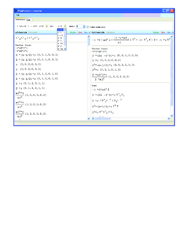
Figure 2: Main window of the application PhysProject

1. The program produces an automatic simplification of the explicit form of elements $o^{\prime}_{I}$ with a given accuracy in the powers of $r$ and calculates the product of any two elements $o^{\prime}_{I},o^{\prime}_{J}$, representing the result in a normal ordering form, when all of the generating elements of the Heisenberg–Weyl superalgebra in the product are written in such a way that the creation operators ($b_{2}^{+},f^{+},b_{1}^{+}$) follow in their writing before the annihilation operators ($b_{2},f,b_{1}$).

2. The problem of collecting similar summands has not yet been completely solved at present due to non-mathematical types of numeric coefficients; however, the program permits one to reduce the opposite summands. To this end, one uses the toggle ”Collect similar items” on the main window of PhysProject.

3. The program produces a visual representation of the obtained results after some choice of the maximal degree on $r$ and elements $o^{\prime}_{1},o^{\prime}_{2}$, whose supercommutator should be verified. Then the result of the left-hand-side window reserved for the $P^{l}_{IJ}$ polynomial (left-hand side value of $[o^{\prime}_{I},o^{\prime}_{J}\}$) in question and the one in the right-hand-side window for the $P^{r}_{IJ}$ (right-hand side value of $[o^{\prime}_{I},o^{\prime}_{J}\}$) with accuracy up to value in ”max r” are computed after calling of the corresponding procedures by means of the buttons ”Calculate”. As a basic way of output of the results, we use a symbolic form which may be chosen from the above-described 3 options in the list ”View” in the top from the right of both the windows.

As a final result of the work of the program, we obtain by a direct comparison of verified expressions from the left- and right-hand sides of the main window that all the relations from the multiplication table 1 for the superalgebra $\mathcal{A}^{\prime}(Y(1),AdS_{d})$ with the elements given by Eqs. (82)–(88) are valid with accuracy up to the fourth power in $r$. Because of a cyclic manner of definition the corresponding polynomials $o^{\prime}_{I}(b_{i}^{+},f^{+},b_{i},f)$ (i.e. following to restricted induction principle), using the program, whose maximal degree is restricted by the value of $q$ in $r^{q}$, we may argue that the multiplication law for the elements of a superalgebra under consideration is true.

5 Conclusions and Perspectives to $\mathcal{A}(Y(k),AdS_{d}),k>1$

In the present work, we have solved a number of problems, which do not seem closely related at first glance, both in a purely algebraic direction and within the area of symbolic computations, which at the same time are related to each other from High Energy Physics considerations.

Initially, we have realized the Verma module $V_{\mathcal{A}^{\prime}}$ construction [33], applied here to the non-linear superalgebra $\mathcal{A}^{\prime}(Y(1),AdS_{d})$ introduced in Ref. [27] and serving a Lagrangian formulation for massive higher-spin spin-tensors in AdS_d-spaces as elements of irreducible AdS-group representation space, characterized by an arbitrary Young tableaux with one row. Within a system of definitions introduced here in order to classify a set of non-linear Lie-type superalgebra, the superalgebra $\mathcal{A}^{\prime}(Y(1),AdS_{d})$ appears by a polynomial superalgebra of order $2$. The construction of Verma module is based on a generalized Cartan procedure following from the fact that negative root vectors ($t^{\prime+}_{1},l^{\prime+}_{2}$) from the maximal Lie subsuperalgebra $osp(2|1)$ in $\mathcal{A}^{\prime}(Y(1),AdS_{d})$ are enlarged by an operator $l^{\prime+}_{1}$ determining the nonlinear part of the latter superalgebra. Formulae (37)–(40), (66)–(70) completely solve the problem of Verma module construction. In the case of the Lie superalgebra $\mathcal{A}^{\prime}(Y(1),\mathbb{R}^{d-1,1})$, we have obtained a new, in comparison with that of Ref. [36] (where it was used the Verma module for $osp(2|1)$ then enlarged to one for $\mathcal{A}^{\prime}(Y(1),\mathbb{R}^{d-1,1})$ by means of dimensional reduction from $\mathbb{R}^{d-1,2}$ to $\mathbb{R}^{d-1,1}$), realization of Verma module, given by Eqs. (37)–(40), (71)–(75). Note that during the investigation of this problem we have obtained some interesting results, such as Odd Pascal triangle, given by Table 2, and determined by the same rules as its standard even analog but with the help of a number of odd-valued combinations (35).

We have realized the Verma module $V_{\mathcal{A}^{\prime}}$ in terms of a formal power series in the degrees of non-supercommuting generating elements $b_{i},b_{i}^{+},f,f^{+},i=1,2$ of a Heisenberg–Weyl superalgebra $A_{1,2}$, whose number coincides with those of negative and positive root vectors in a Cartan-like decomposition for the superalgebra $\mathcal{A}^{\prime}(Y(1),AdS_{d})$. This problem is completely described by the formulae (82)–(88). The corresponding oscillator realization for the Lie superalgebra $\mathcal{A}^{\prime}(Y(1),\mathbb{R}^{d-1,1})$ has a polynomial form given by Eqs. (82), (83), (94)–(96), which follows as a consequence from the previous relations for a vanishing inverse squared AdS_d-space radius $r$.

On a programming level, we have solved the third problem of the paper by means of finding an explicit formalized representation for the superalgebra $\mathcal{A}^{\prime}(Y(1),AdS_{d})$ in terms of a so-called formal setting of the algorithm, which translates the results of the Verma module $V_{\mathcal{A}^{\prime}}$ realization over a Heisenberg–Weyl superalgebra in a set of formalized relations (99)–(2.2). It is the relations which, together with the multiplication table 1 and the explicit form of the basis operators of the superalgebra $\mathcal{A}^{\prime}(Y(1),AdS_{d})$ (82)–(88), have become the main relations to realize the programming data model in the language C# within the symbolic computation approach.

We have suggested a two-level program model which permits one to realize, on a programming level, all the properties of an arbitrary superalgebra of polynomials with an associative multiplication law as a basic model of superalgebra, and those of proper superalgebra of polynomials from $\mathcal{A}^{\prime}(Y(1),AdS_{d})$ (restricted by the value of exponent $q$ in $r^{q}$) as a polynomial superalgebra model. It is shown that in order to describe, in the programming language C#, an arbitrary polynomial of finite power in $r$, it is sufficient to use five basic classes Expression, Coefficient, Literal, Product and Sum from the first level and one class PhysEnvironment from the second level, that is illustrated by Figure 1.

We have developed, on a basis of a two-level programming model, a computer program in C#, whose main window is shown by Figure 2, and which verifies the fact that the operators of the superalgebra $\mathcal{A}^{\prime}(Y(1),AdS_{d})$ satisfy the given algebraic supercommutator relations by means of a restricted induction principle with a parameter being the exponent of the inverse squared radius $r$ of the AdS_d-space. The validity of the multiplication table 1 is established up to the fourth power in $r$, which is due to the cyclic character of definitions of the operators $\mathcal{A}^{\prime}(Y(1),AdS_{d})$ in the powers of $r$ practically guarantees the solution of the verification problem for $q\geq 5$ in $r^{q}$.

The algorithm, basic data structures, the methods of their processing and the solution of the formalized problem compose the basic results of this part of the paper.

Among possible perspectives of research within algebraic and symbolic computations, we note the problems of constructing Verma modules and their oscillator realizations for more involved non-linear algebras and superalgebras corresponding to higher-spin fields in the AdS_d-space subject to a multi-row Young tableaux, which were discussed in Ref. [47] for the algebra $\mathcal{A}^{\prime}(Y(2),AdS_{d})$. This will be by the purpose of a forthcoming work [49]. Of course, a detailed verification of the validity of the corresponding multiplication table of the resulting expressions for operators of those (super)algebras within the symbolic computations approach will be a topical problem as well.

As to the development of the program PhysProject, one may specify some directions. First of all, it is an improvement of the visual presentation of data. Second, the nearest way to enhance the program code of the existing program model is the swap-out of the second level of data model and a distribution of the methods to new classes with respect to those of the first-level model, or an inheritance of the latter classes and an accumulation of methods.

The general direction of an enhancement of the program consists in the increasing of its universality in order to adapt the application of the program to other non-linear algebraic structures. To these items one may relate a standardization of the declaration of explicit forms of basis elements such as $o^{\prime}_{I}$, and a definition of multiplication tables, of the rules for commutation relations. This will permit one to apply the program to more involved non-linear algebras and superalgebras and resolve the problem of attaching the program to concrete superalgebras.

Finally, it is worth noting that our program is assigned to work with more general objects then $GR$-algebras and corresponding Gröbner bases (see Refs. [52, 53] and references therein). At the same time, it is interesting to establish a more detailed correspondence with these structures and corresponding program systems for their treatment such as Plural, system OpenXM [54].

References

• [1] A.O. Barut and R. Ronchka, The theory of group representations and its applications, (PWN, Warsaw), 1977.
• [2] D.Leites, Lie superalgebras, JOSMAR (J.Soviet Math.) 30 (1985) 2481.
• [3] V. Dolotin and A. Morozov, Introduction to Non-Linear Algebra, World Scientific, 2007, [arXiv:hep-th/0609022].
• [4] K. Schoutens, A.Sevrin and P. van Nieuwenhuizen, Quantum BRST Charge for Quadratically Nonlinear Lie Algebras, Commun. Math. Phys. 124 (1989) 87–103; C.N.Pope, Lectures on W algebras and W gravity, [arXiv:hep-th/9112076].
• [5] E. Witten, Noncommutative geometry and string field theory, Nucl.Phys. B268 (1986) 253; C.B. Torn, String field thoory, Phys.Repts 175 (1989) 1–101; W. Taylor, B. Zwiebach, D-branes, tachyons and string field theory, [arXiv:hep-th/0311017].
• [6] M. Vasiliev, Higher spin gauge theories in various dimensions, Fortsch. Phys. 52 (2004) 702–717, [arXiv:hep-th/0401177]; D. Sorokin, Introduction to the classical theory of higher spins, AIP Conf. Proc. 767 (2005) 172–202, [arXiv:hep-th/0405069]; N. Bouatta, G. Compère, A. Sagnotti, An introduction to free higher-spin fields, [arXiv:hep-th/0409068]; A. Sagnotti, E. Sezgin, P. Sundell, On higher spins with a strong Sp(2,R) condition, [arXiv:hep-th/0501156]; X. Bekaert, S. Cnockaert, C. Iazeolla, M.A. Vasiliev, Nonlinear higher spin theories in various dimensions, [arXiv:hep-th/0503128].
• [7] C. Fronsdal, Singletons and massless, integer-spin fileds on de Sitter space, Phys. Rev. D20 (1979) 848-856; J. Fang, C. Fronsdal, Massless, half-integer-spin fields in de Sitter space, Phys. Rev. D22 (1980) 1361–1367; M.A. Vasiliev, Free massless fermionic fields of arbitrary spin in D-dimensional anti-de Sitter space, Nucl. Phys. B301 (1988) 26–51; V.E. Lopatin, M.A. Vasiliev, Free massless bosonic fields of arbitrary spin in D-dimensional de Sitter space, Mod. Phys. Lett. A3 (1998) 257–265.
• [8] E.S. Fradkin, M.A. Vasiliev, Cubic Interaction In Extended Theories Of Massless Higher Spin Fields, Nucl. Phys. B 291 (1987) 141; Candidate To The Role Of Higher Spin Symmetry, Annals Phys. 177 (1987) 63; On The Gravitational Interaction Of Massless Higher Spin Fields, Phys. Lett. B 189 (1987) 89–95; M. A. Vasiliev, Consistent equation for interacting gauge fields of all spins in (3+1)-dimensions, Phys. Lett. B 243 (1990) 378–382; Cubic interactions of bosonic higher spin gauge fields in AdS(5), Nucl. Phys. B 616 (2001) 106–162 [Erratum-ibid. B 652 (2003) 407] [arXiv:hep-th/0106200]; Algebraic aspects of the higher spin problem, Phys. Lett. B 257 (1991) 111–118; More on equations of motion for interacting massless fields of all spins in (3+1)-dimensions, Phys. Lett. B 285 (1992) 225–234; Class. Quant. Grav. 8, (1991) 1387; Nonlinear equations for symmetric massless higher spin fields in (A)dS(d), Phys. Lett. B 567 (2003) 139–151, [arXiv:hep-th/0304049].
• [9] E, Sezgin, P. Sundell, Holography in 4D (super)higher spin theories and a test via cubic scalar couplings, JHEP 0507 (2005) 044, [arXiv:hep-th/0305040].
• [10] A.O. Barvinsky, A.Yu. Kamenshchik and A.A. Starobinsky, Inflation scenario via the Standard Model Higgs boson and LHC, JCAP 0811 (2008) 021, [arXiv:0809.2104[hep-ph]].
• [11] N. Beisert, M. Bianchi, J.F. Morales and H. Samtleben, Higher spin symmetries and N=4 SYM, JHEP 0407 (2004) 058, [arXiv:hep-th/0405057]; A.C. Petkou, Holography, duality and higher spin fields, [arXiv:hep-th/0410116]; M. Bianchi, P.J. Heslop, F. Riccioni, More on la Grande Bouffe: towards higher spin symmetry breaking in AdS, JHEP 0508 (2005) 088, [arXiv:hep-th/0504156].
• [12] G. Bonelli, On the boundary gauge dual of closed tensionless free strings in AdS, JHEP 0411 (2004) 059, [arXiv:hep-th/0407144]; On the covariant quantization of tensionless bosonic strings in AdS spacetime, JHEP 0311 (2003) 028, [arXiv:hep-th/0309222]; On the tensionless limit of bosonic strings, infinite symmetries and higher spins, Nucl. Phys. B669 (2003) 159–172, [arXiv:hep-th/0305155].
• [13] J.M. Maldacena, The large N limit of superconformal field theories and supergravity, Adv. Theor. Math. Phys. 2 (1998) 231, [arXiv:hep-th/9711200].
• [14] S. Weinberg, The Quantum Theory of fields. Vol. 1: Foundations, Cambridge, UK Univercity Press, 1995, 609.
• [15] D.M. Gitman and I.V. Tyutin, Quantization of Fields with Constraints, Springer-Verlag, 1990, 288.
• [16] M. Fierz, W. Pauli, On relativistic wave equations for particles of arbitrary spin in an electromagnetic field, Proc.R.Soc.London, Ser. A, 173 (1939) 211–232; L.P.S. Singh, C.R. Hagen, Lagrangian formulation for arbitrary spin. 1. The bosonic case, Phys. Rev. D9 (1974) 898–909; Lagrangian formulation for arbitrary spin. 2. The fermionic case, Phys. Rev. D9 (1974) 910–920.
• [17] R.R. Metsaev, Fermionic fields in the d-dimensional anti-de Sitter space-time, Phys.Lett. B419 (1998) 49–56, [arXiv:hep-th/9802097]; Massless mixed symmetry bosonic free fields in d-dimensional anti-de Sitter space-time, Phys. Lett. B354 (1995) 78–84.
• [18] M.A. Vasiliev, ’Gauge’ Form Of Description Of Massless Fields With Arbitrary Spin, (In Russian). Sov. J. Nucl. Phys. 32 (1980) 439.
• [19] K.B. Alkalaev, O.V. Shaynkman and M.A. Vasiliev, On the frame - like formulation of mixed symmetry massless fields in (A)dS(d), Nucl. Phys. B692 (2004) 363–393, [arXiv:hep-th/0311164].
• [20] G. Barnich and M. Grigoriev, Parent form for higher spin fields on anti-de Sitter space, JHEP 08 (2006) 013, [arXiv:hep-th/0602166]; K. Alkalaev, M. Grigoriev and I. Tipunin, Massless Poincare modules and gauge invariant equations, Preprint FIAN/TD/23/08 [arXiv:0811.3999[hep-th]].
• [21] M.A. Vasiliev, Equations Of Motion Of Interacting Massless Fields Of All Spins As A Free Differential Algebra, Phys. Lett. B209 (1988) 491–497; M. A. Vasiliev, Consistent equations for interacting massless fields of all spins in the first order in curvatures, Annals Phys. 190 (1989) 59 -106.
• [22] C. Fronsdal, Massless Fields with Integer Spin, Phys. Rev. D18 (1978) 3624.
• [23] Yu.M. Zinoviev, On Massive Mixed Symmetry Tensor Fields in Minkowski space and (A)dS, [arXiv:hep-th/0211233].
• [24] D. Francia, A. Sagnotti, Free geometric equations for higher spins, Phys. Lett. B543 (2002) 303–310, [arXiv:hep-th/0207002].
• [25] C. Becchi, A. Rouet and R. Stora, Comm. Math. Phys. 42 (1975) 127;
I.V. Tyutin, Gauge invariance in field theory and statistical physics in operator formalism, Preprint Lebedev Inst. No. 39 (1975), [arXiv:0812.0580[hep-th]].
• [26] I.A. Batalin, E.S. Fradkin, Operator quantizatin method and abelization of dynamical systems subject to first class constraints, Riv. Nuovo Cimento, 9, No 10 (1986) 1; I.A. Batalin, E.S. Fradkin, Operator quantization of dynamical systems subject to constraints. A further study of the construction, Ann. Inst. H. Poincare, A49 (1988) 145; M. Henneaux, C. Teitelboim, Quantization of Gauge Systems, Princeton Univ. Press, 1992.
• [27] I.L. Buchbinder, V.A. Krykhtin, A.A. Reshetnyak, BRST approach to Lagrangian construction for fermionic higher spin fields in AdS space, Nucl. Phys. B787 (2007) 211-240, [arXiv:hep-th/0703049].
• [28] Choon-Lin Ho and T. Tanaka, Simultaneous ordinary and type A N-fold supersymmetries in Schr odinger, Pauli, and Dirac equations, Ann. Phys. 321 (2006) 1375–1407, [arXiv:hep-th/0509020]; [arXiv:hep-th/0212276]; Parasupersymmetry and N-fold Supersymmetry in Quantum Many-Body Systems I. General Formalism and Second Order, Ann. Phys. 322 (2007) 2350–2373. [arXiv:hep-th/0610311];Parasupersymmetry and N-fold Supersymmetry in Quantum Many-Body Systems II. Third Order, Ann. Phys. 322 (2007) 2682, [arXiv:hep-th/0612263].
• [29] N. Mohammedi, G. Moultaka, and M.R. de Traubenberg, Field theoretic realizations for cubic supersymmetry, Int. J. Mod. Phys. A 19 (2004) 5585–5608, [arXiv:hep-th/0305172].
• [30] M. Plyushchay, Hidden nonlinear supersymmetries in pure parabosonic systems Int.J.Mod.Phys. A15 (2000) 3679–3698, [arXiv:hep-th/9903130]; S.M. Klishevich and M.S. Plyushchay, Nonlinear supersymmetry, quantum anomaly and quasiexactly solvable systems, Nucl.Phys. B606 (2001) 583–612, [arXiv:hep-th/0012023].
• [31] C. Leivaa and M.S. Plyushchay, Superconformal mechanics and nonlinear supersymmetry, JHEP 0310 (2003) 069, [arXiv:hep-th/0304257]; A. Anabalon and M.S. Plyushchay, Interaction via reduction and nonlinear superconformal symmetry, Phys.Lett. B572 (2003) 202–209, [arXiv:hep-th/0306210]; Bosonized supersymmetry from the Majorana-Dirac-Staunton theory, and massive higher-spin fields. By Peter A. Horvathy, Mikhail S. Plyushchay, Mauricio Valenzuela. Phys.Rev.D77:025017,2008, [arXiv:0710.1394[hep-th]].
• [32] F. Correa, V. Jakubsky, L.-M. Nieto, M.S. Plyushchay, Self-isospectrality, special supersymmetry, and their effect on the band structure, Phys. Rev. Lett. 101 (2008) 030403, [arXiv:0801.1671[hep-th]]; F. Correa, V. Jakubsky and M.S. Plyushchay, Finite-gap systems, tri-supersymmetry and self-isospectrality, J.Phys. A41 (2008) 485303 [arXiv:0806.1614[hep-th]]; Aharonov-Bohm effect on AdS(2) and nonlinear supersymmetry of reflectionless Poschl-Teller system, Ann. Phys. 324 (2009) 1078–1094, [arXiv:0809.2854[hep-th]].
• [33] J. Dixmier, Algebres enveloppantes, Gauthier-Villars, Paris (1974).
• [34] L.D. Faddeev, S.L. Shatashvili, Realization of the Schwinger term in the Gauss law and the possibility of correct quantization of a theory with anomalies, Phys.Lett. B167 (1986) 225–238; I.A. Batalin, E.S. Fradkin, T.E. Fradkina, Another version for operatorial quantization of dynamical systems with iireducible constraints, Nucl. Phys. B314 (1989) 158–174; I.A. Batalin, I.V. Tyutin, Existence theorem for the effective gauge algebra in the generalized canonical formalism and Abelian conversion of second class constraints, Int. J. Mod. Phys. A6 (1991) 3255–3282; E. Egorian, R. Manvelyan, Quantization of dynamical systems with first and second class constraints, Theor. Math. Phys. 94 (1993) 241–252.
• [35] C. Burdik, Realizations of the real simple Lie algebras: the method of construction, J. Phys. A: Math. Gen. 18 (1985) 3101–3112.
• [36] I.L. Buchbinder, V.A. Krykhtin, L.L. Ryskina, H. Takata, Gauge invariant Lagrangian construction for massive higher spin fermionic fields, Phys. Lett. B641 (2006) 386, [arXiv:hep-th/0603212].
• [37] P.Yu. Moshin, A.A. Reshetnyak, BRST approach to Lagrangian formulation for mixed-symmetry fermionic higher-spin fields, JHEP, 10 (2007) 040, [arXiv:0706.0386[hep-th]].
• [38] C. Burdik, O. Navratil, A. Pashnev, On the Fock Space Realizations of Nonlinear Algebras Describing the High Spin Fields in AdS Spaces, [arXiv: hep-th/0206027].
• [39] I.L. Buchbinder, V.A. Krykhtin, P.M. Lavrov, Gauge invariant Lagrangian formulation of higher spin massive bosonic field theory in AdS space, Nucl.Phys. B762 (2007) 344, [arXiv:hep-th/0608005].
• [40] V. Levandovskyy and Jorge Morales Computational D-module with Singular, Comparison with Other Systems and Two New Algorithms, In Proceedings of the Int. Symposium on Symbolic and Algebraic Computation (ISSAC’08). ACM Press (2008); V. Levandovskyy, Plural, a Non-commutative Extension of Singular: Past, Present and Future, In A. Iglesias, N. Takayama: Proceedngs of the Int. Symposium on Mathematical Theory of Networks and System (MTNS’06), 2006. .
• [41] PLURAL - a kernel extension of SINGULAR .Available from http://www.singular.uni-kl.de/plural/overview.html.
• [42] V. Levandovskyy, On Preimages of Ideals in Certain Non-commutative Algebras, Computational Commut. and Non-Commut. Algebraic Geometry, Eds. S.Cojocaru, G.Pfisher, (IOS Press) 2005 44–62.
• [43] M. Asoreya, P.M. Lavrov, O.V. Radchenko and A. Sugamoto, BRST structure of non-linear superalgebras, [arXiv:0809.3322[hep-th]].
• [44] I.L. Buchbinder and P.M. Lavrov, Classical BRST charge for nonlinear algebras, J. Math. Phys. 48 No. 8 (2007) 082306-1-15 [arXiv:hep-th/0701243]; A.P. Isaev, S.O. Krivonos and O.V. Ogievetsky, BRST operators for W algebras, Math.Phys. 49 (2008) 073512, [arXiv:0802.3781[math-ph]].
• [45] M. Henneaux, Hamiltonian form of the path integral for theories with a gauge freedom, Phys. Rept. 126 (1985) 1–66.
• [46] A. Dresse and M. Henneaux, BRST structure of polynomial Poisson algebras, J. Math. Phys. 35 (1994) 1334, [arXiv:hep-th/9312183].
• [47] A.A. Reshetnyak, Nonlinear Operator Superalgebras and BFV-BRST Operators for Lagrangian Description of Mixed-symmetry HS Fields in AdS Spaces, [arXiv:0812.2329[hep-th]].
• [48] P.Yu. Moshin and A.A. Reshetnyak, in preparation.
• [49] A.A. Reshetnyak, in preparation.
• [50] R. Howe, Transcending classical invariant theory, J. Amer. Math. Soc. 3 (1989); Remarks on classical invariant theory, Trans. Amer. Math. Soc. 2 (1989) 313.
• [51] K. Alkalaev, M. Grigoriev, and I. Tipunin, Massless Poincar e modules and gauge invariant equations, [arXiv:0811.3999[hep-th]].
• [52] V. Levandovskyy and E. Zerz, Algebraic systems theory and computer algebraic methods for some classes of linear control systems. In Proc. of the International Symposium on Mathematical Theory of Networks and Systems (MTNS 06), 2006.
• [53] T. Mora, An introduction to commutative and non-commutative Groebner bases. Theor. Comp. Sci., 134 (1994) 131 -173.
• [54] N. Takayama, kan/sm1, a Gröbner engine for the ring of differential and difference operators, 2003. Available from http://www.math.kobe-u.ac.jp/KAN/index.html.
• [55] A.A. Reshetnyak, ”BFV-BRST operators and Fock space realizations of Verma modules for non-linear superalgebras underlying Lagrangian formulations for mixed-symmetry HS fields in AdS spaces”, on-line Proc. 4th Int. Sakharov Conf., Moscow, May, 18-23, 2009, $\verb"http://sci4.lpi.ru/proc_strings.htm"$