Statistical properties and decoherence of two-mode photon-subtracted squeezed vacuum

Abstract

We investigate the statistical properties of the photon-subtractions from the two-mode squeezed vacuum state and its decoherence in a thermal environment. It is found that the state can be considered as a squeezed two-variable Hermite polynomial excitation vacuum and the normalization of this state is the Jacobi polynomial of the squeezing parameter. The compact expression for Wigner function (WF) is also derived analytically by using the Weyl ordered operators’ invariance under similar transformations. Especially, the nonclassicality is discussed in terms of the negativity of WF. The effect of decoherence on this state is then discussed by deriving the analytical time evolution results of WF. It is shown that the WF is always positive for any squeezing parameter and photon-subtraction number if the decay time exceeds an upper bound ($\kappa t>\frac{1}{2}\ln\frac{2\bar{n}+2}{2\bar{n}+1}).$

Key Words: photon-subtraction; nonclassicality; Wigner function; negativity; two-mode squeezed vacuum state

PACS numbers: 03.65.Yz, 42.50.Dv

I Introduction

Entanglement is an important resource for quantum information 1 . In a quantum optics laboratory, Gaussian states, being characteristic of Gaussian Wigner functions, have been generated but there is some limitation in using them for various tasks of quantum information procession 2 . For example, in the first demonstration of continuous variables quantum teleportation (two-mode squeezed vacuum state as a quantum channel), the squeezing is low, thus the entanglement of the quantum channel is such low that the average fidelity of quantum teleportation is just more $\left(8\pm 2\right)\%$ than the classical limits. In order to increase the quantum entanglement there have been suggestions and realizations to engineering the quantum state by subtracting or adding photons from/to a Gaussian field which are plausible ways to conditionally manipulate nonclassical state of optical field 2a ; 2b ; 2c ; 2d ; 2e ; 2f ; 2g . In fact, such methods allowed the preparation and analysis of several states with negative Wigner functions, including one- and two-photon Fock states 3 ; 4 ; 5 ; 6 , delocalized single photons 7 ; 8 , and photon-subtracted squeezed vacuum states (PSSV), very similar to quantum superpositions of coherent states with small amplitudes (a Schrödinger kitten state 9 ; 10 ; 11 ; 12 ) for single-mode case.

Recently, the two-mode PSSVs (TPSSVs) have been paid enough attention by both experimentalists and theoreticians 3 ; 4 ; 13 ; 14 ; 15 ; 16 ; 17 ; 18 ; 19 ; 20 ; 21 ; 22 . Olivares et al 13 ; 14 considered the photon subtraction using on–off photodetectors and showed the improvement of quantum teleportation depending on various parameters involved. Then they further studied the nonlocality of photon subtraction state in the presence of noise 15 . Kitagawa et al 16 , on the other hand, investigated the degree of entanglement for the TPSSV by using an on-off photondetector. Using operation with single photon counts, Ourjoumtsev et al .3 ; 4 have demonstrated experimentally that the entanglement between Gaussian entangled states, can be increased by subtracting only one photon from two-mode squeezed vacuum states. The resulted state is a complex quantum state with a negative two-mode Wigner function. However, so far as we know, there is no report about the nonclassicality and decoherence of TPSSV for arbitrary number PSSV in literature before.

In this paper, we will explore theoretically the statistical properties and decoherence of arbitrary number TPSSV. This paper is arranged as follows: in Sect. II we introduce the TPSSV, denoted as $a^{m}b^{n}S_{2}(\lambda)\left|00\right\rangle,$ where $S_{2}(\lambda)$ is two-mode squeezing operator with $\lambda$ being squeezing parameter and $m,n$ are the subtracted photon number from $S_{2}(\lambda)\left|00\right\rangle$ for mode $a$ and $b$, respectively. It is found that it is just a squeezed two-variable Hermite polynomial excitation on the vacuum state, and then the normalization factor for $a^{m}b^{n}S_{2}(\lambda)\left|00\right\rangle$ is derived, which turns out to be a Jacobi polynomial, a remarkable result. In Sec. III, the quantum statistical properties of the TPSSV, such as distribution of photon number, squeezing properties, cross-correlation function and antibunching, are calculated analytically and then be discussed in details. Especially, in Sec. IV, the explicit analytical expression of Wigner function (WF) of the TPSSV is derived by using the Weyl ordered operators’ invariance under similar transformations, which is related to the two-variable Gaussian-Hermite polynomials, and then its nonclassicality is discussed in terms of the negativity of WF which implies the highly nonclassical properties of quantum states. Sec. V is devoted to studying the effect of the decoherence on the TPSSV in a thermal environment. The analytical expressions for the time-evolution of the state and its WF are derived, and the loss of nonclassicality is discussed in reference of the negativity of WF due to decoherence. We find that the WF for TPSSV has no chance to present negative value for all parameters $\lambda$ and $m,n$ if the decay time $\kappa t>\frac{1}{2}\ln\frac{2\bar{n}+2}{2\bar{n}+1}\$(see Eq.(46) below), where $\bar{n}$ denotes the average thermal photon number in the environment with dissipative coefficient $\kappa$.

II Two-mode photon-subtracted squeezed vacuum states

II.1 TPSSV as the squeezed two-variable Hermite polynomial excitation state

The definition of the two-mode squeezed vacuum state is given by

$$S_{2}(\lambda)\left|00\right\rangle=\text{sech}\lambda\exp(a^{\dagger}b^{\dagger}\tanh\lambda)\left|00\right\rangle,$$ (1)

where $S_{2}(\lambda)=\exp[\lambda(a^{\dagger}b^{\dagger}-ab)]$ is the two-mode squeezing operator 23 ; 24 ; 25 with $\lambda$ being a real squeezing parameter, and $a$, $b$ are the Bose annihilation operators, $[a,a^{\dagger}]=[b,b^{\dagger}]=1$. Theoretically, the TPSSV can be obtained by repeatedly operating the photon annihilation operator $a$ and $b$ on $S_{2}(\lambda)\left|00\right\rangle$, defined as

$$\left|\lambda,m,n\right\rangle=a^{m}b^{n}S_{2}(\lambda)\left|00\right\rangle,$$ (2)

where $\left|\lambda,m,n\right\rangle$ is an un-normalization state. Noticing the transform relations,

$$S_{2}^{\dagger}(\lambda)aS_{2}(\lambda) =a\cosh\lambda+b^{\dagger}\sinh\lambda,$$

$$S_{2}^{\dagger}(\lambda)bS_{2}(\lambda) =b\cosh\lambda+a^{\dagger}\sinh\lambda,$$ (3)

we can reform Eq.(2) as

$$\left|\lambda,m,n\right\rangle =S_{2}(\lambda)S_{2}^{\dagger}(\lambda)a^{m}b^{n}S_{2}(\lambda)\left|00\right\rangle$$

$$=S_{2}(\lambda)(a\cosh\lambda+b^{\dagger}\sinh\lambda)^{m}(b\cosh\lambda+a^{\dagger}\sinh\lambda)^{n}\left|00\right\rangle$$

$$=S_{2}(\lambda)\sinh^{n+m}\lambda\sum_{l=0}^{m}\frac{m!\coth^{l}\lambda}{l!\left(m-l\right)!}b^{\dagger m-l}a^{l}a^{\dagger n}\left|00\right\rangle.$$ (4)

Further note that $a^{\dagger n}\left|0\right\rangle=\sqrt{n!}\left|n\right\rangle$ and $a^{l}\left|n\right\rangle=\frac{\sqrt{n!}}{\sqrt{(n-l)!}}\left|n-l\right\rangle=\frac{\sqrt{n!}}{(n-l)!}a^{\dagger n-l}\left|0\right\rangle$, leading to $a^{l}a^{\dagger n}\left|00\right\rangle=\frac{n!}{(n-l)!}a^{\dagger n-l}\left|00\right\rangle$, thus Eq.(4) can be re-expressed as

$$\left|\lambda,m,n\right\rangle =S_{2}(\lambda)\sinh^{n+m}\lambda\sum_{l=0}^{\min\left(m,n\right)}\frac{m!n!\coth^{l}\lambda}{l!\left(m-l\right)!(n-l)!}a^{\dagger n-l}b^{\dagger m-l}\left|00\right\rangle$$

$$=\frac{\sinh^{\left(n+m\right)/2}2\lambda}{\left(i\sqrt{2}\right)^{n+m}}S_{2}(\lambda)\sum_{l=0}^{\min(m,n)}\frac{(-1)^{l}n!m!\left(i\sqrt{\tanh\lambda}b^{\dagger}\right)^{m-l}\left(i\sqrt{\tanh\lambda}a^{\dagger}\right)^{n-l}}{l!(n-l)!\left(m-l\right)!}\left|00\right\rangle$$

$$=\frac{\sinh^{\left(n+m\right)/2}2\lambda}{\left(i\sqrt{2}\right)^{n+m}}S_{2}(\lambda)H_{m,n}\left(i\sqrt{\tanh\lambda}b^{\dagger},i\sqrt{\tanh\lambda}a^{\dagger}\right)\left|00\right\rangle,$$ (5)

where in the last step we have used the definition of the two variables Hermitian polynomials 26 ; 27 , i.e.,

$$H_{m,n}\left(\epsilon,\varepsilon\right)=\sum_{k=0}^{\min\left(m,n\right)}\frac{\left(-1\right)^{k}m!n!\epsilon^{m-k}\varepsilon^{n-k}}{k!(m-k)!(n-k)!}.$$ (6)

From Eq.(5) one can see clearly that the TPSSV $\left|\lambda,m,n\right\rangle$ is equivalent to a two-mode squeezed two-variable Hermite-excited vacuum state and exhibits the exchanging symmetry, namely, interchanging $m\Leftrightarrow n$ is equivalent to $a^{\dagger}\Leftrightarrow b^{\dagger}$. It is clear that, when $m=n=0,$ Eq.(5) just reduces to the two-mode squeezed vacuum state due to $H_{0,0}=1$; while for $n\neq 0$ and $m=0,$ noticing $H_{0,n}\left(x,y\right)=y^{n},$ Eq.(5) becomes ($N_{\lambda,0,n}^{-1}=n!\sinh^{2n}\lambda)$, see Eq.(11) below) $\left|\lambda,0,n\right\rangle=S_{2}(\lambda)\left|n,0\right\rangle,$which is just a squeezed number state, corresponding to a pure negative binomial state 28 .

II.2 The normalization of $\left|\lambda,m,n\right\rangle$

To know the normalization factor $N_{\lambda,m,n}$ of $\left|\lambda,m,n\right\rangle$, let us first calculate the overlap $\left\langle\lambda,m+s,n+t\right.\left|\lambda,m,n\right\rangle$. For this purpose, using the first equation in Eq.(5) one can express $\left|\lambda,m,n\right\rangle$ as

$$\left|\lambda,m,n\right\rangle=S_{2}(\lambda)\sum_{l=0}^{\min(m,n)}\frac{m!n!\sinh^{n+m}\lambda\coth^{l}\lambda}{l!\sqrt{(m-l)!(n-l)!}}\left|n-l,m-l\right\rangle,$$ (7)

which leading to

$$\left\langle\lambda,m+s,n+t\right.\left|\lambda,m,n\right\rangle$$

$$=m!\left(n+s\right)!\delta_{s,t}\sinh^{2n+2m+2s}\lambda$$

$$\times\sum_{l=0}^{\min(m,n)}\frac{\left(m+s\right)!n!\coth^{2l+s}\lambda}{l!(m-l)!(n-l)!(l+s)!},$$ (8)

where $\delta_{s,t}$ is the Kronecker delta function. Without lossing the generality, supposing $m<n$ and comparing Eq.(8) with the standard expression of Jacobi polynomials 29

$$P_{m}^{(\alpha,\beta)}(x)=\left(\frac{x-1}{2}\right)^{m}\sum_{k=0}^{m}\left(\begin{array}[c]{c}m+\alpha\\ k\end{array}\right)\left(\begin{array}[c]{c}m+\beta\\ m-k\end{array}\right)\left(\frac{x+1}{x-1}\right)^{k},$$ (9)

one can put Eq.(8) into the following form

$$\left\langle\lambda,m+s,n+t\right.\left|\lambda,m,n\right\rangle=m!\left(n+s\right)!\delta_{s,t}\sinh^{2n+s}\lambda\cosh^{s}\lambda P_{m}^{(n-m,s)}(\allowbreak\cosh 2\lambda),$$ (10)

which is just related to Jacobi polynomials. In particular, when $s=t=0$, the normalization constant $\emph{N}_{m,n,\lambda}$ for the state $\left|\lambda,m,n\right\rangle$ is given by

$$N_{\lambda,m,n}=\left\langle\lambda,m,n\right.\left|\lambda,m,n\right\rangle=m!n!\sinh^{2n}\lambda P_{m}^{(n-m,0)}(\cosh 2\lambda),$$ (11)

which is important for further studying analytically the statistical properties of the TPSSV. For the case $m=n$, it becomes Legendre polynomial of the squeezing parameter $\lambda$, because of $P_{n}^{(0,0)}(x)=P_{n}(x),$ $P_{0}(x)=1$; while for $n\neq 0$ and $m=0,$ noticing that $P_{0}^{(n,0)}(x)=1$ then $N_{\lambda,0,n}=n!\sinh^{2n}\lambda.$ Therefore, the normalized TPSSV is

$$\left|\left|\lambda,m,n\right\rangle\right.\equiv\left[m!n!\sinh^{2n}\lambda P_{m}^{(n-m,0)}(\cosh 2\lambda)\right]^{-1/2}a^{m}b^{n}S_{2}(\lambda)\left|00\right\rangle.$$ (12)

From Eqs. (2) and (11) we can easily calculate the average photon number in TPSSV (denoting $\tau=\cosh 2\lambda$),

$$\left\langle a^{\dagger}a\right\rangle =N_{\lambda,m,n}^{2}\left\langle 00\right|S_{2}^{{\dagger}}(\lambda)a^{{\dagger}m+1}b^{{\dagger}n}a^{m+1}b^{n}S_{2}(\lambda)\left|00\right\rangle$$

$$=\left(m+1\right)\frac{P_{m+1}^{(n-m-1,0)}(\tau)}{P_{m}^{(n-m,0)}(\tau)},$$ (13)

$$\left\langle b^{\dagger}b\right\rangle =\left(n+1\right)\sinh^{2}\lambda\frac{P_{m}^{(n-m+1,0)}(\tau)}{P_{m}^{(n-m,0)}(\tau)}.$$ (14)

In a similar way we have

$$\left\langle a^{\dagger}b^{\dagger}ab\right\rangle=\left(m+1\right)\left(n+1\right)\sinh^{2}\lambda\frac{P_{m+1}^{(n-m,0)}(\tau)}{P_{m}^{(n-m,0)}(\tau)}.$$ (15)

Thus the cross-correlation function $g_{12}^{(2)}$ can be obtained by 30 ; 31 ; 32

$$g_{12}^{(2)}(\lambda) =\frac{\left\langle a^{\dagger}b^{\dagger}ab\right\rangle}{\left\langle a^{\dagger}a\right\rangle\left\langle b^{\dagger}b\right\rangle}$$

$$=\frac{P_{m+1}^{(n-m,0)}(\tau)}{P_{m+1}^{(n-m-1,0)}(\tau)}\frac{P_{m}^{(n-m,0)}(\tau)}{P_{m}^{(n-m+1,0)}(\tau)}.$$ (16)

Actually, the cross-correlation between the two modes reflects correlation between photons in two different modes, which plays a key role in rendering many two-mode radiations nonclassically. In Fig.1, we plot the graph of $g_{12}^{(2)}\left(\lambda\right)$ as the function of $\lambda$ for some different ($m,n$) values. It is shown that $g_{12}^{(2)}\left(\lambda\right)$ are always larger than unit, thus there exist correlations between the two modes. We emphasize that the WF has negative region for all $\lambda,$ and thus the TPSSV is nonclassical. In our following work, we pay attention to the ideal TPSSV.

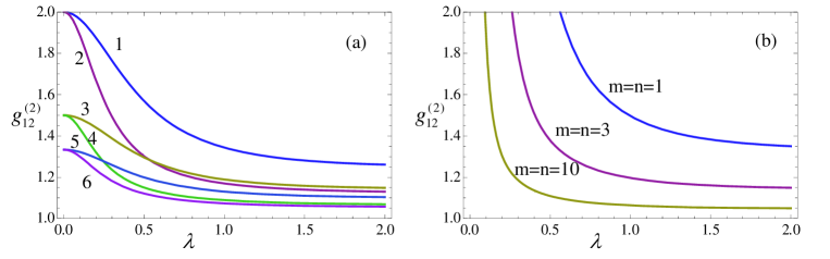
Figure 1: (Color online) Cross-correlation function between the two modes $a$ and $b$ as a function of $\lambda$ for different parameters ($m,n$). The number 1,2,3,4,5,6 in (a) denote that ($m,n$) are eauql to (1,2), (3,4), (2,4),(6,8),(3,6) and (7,10) respectively.

III Quantum statistical properties of the TPSSV

III.1 Squeezing properties

For a two-mode system, the optical quadrature phase amplitudes can be expressed as follows:

$$Q=\frac{Q_{1}+Q_{2}}{\sqrt{2}},\text{ }P=\frac{P_{1}+P_{2}}{\sqrt{2}},\text{ }[Q,P]=\mathtt{i},$$ (17)

where $Q_{1}=(a+a^{\dagger})/\sqrt{2}$, $P_{1}=(a-a^{\dagger})/(\sqrt{2}\mathtt{i})$, $Q_{2}=(b+b^{\dagger})/\sqrt{2}$ and $P_{2}=(b-b^{\dagger})/(\sqrt{2}\mathtt{i})$ are coordinate- and momentum- operator, respectively. Their variances are $(\Delta Q)^{2}=\left\langle Q^{2}\right\rangle-\left\langle Q\right\rangle^{2}$ and $(\Delta P)^{2}=\left\langle P^{2}\right\rangle-\left\langle P\right\rangle^{2}$. The phase amplifications satisfy the uncertainty relation of quantum mechanics $\Delta Q\Delta P\geq 1/2$. By using Eqs.(10) and (11), it is easy to see that $\left\langle a\right\rangle=\left\langle a^{\dagger}\right\rangle=\left\langle b\right\rangle=\left\langle b^{\dagger}\right\rangle=0\$and $\left\langle a^{2}\right\rangle=\left\langle a^{\dagger 2}\right\rangle=\left\langle b^{2}\right\rangle=\left\langle b^{\dagger 2}\right\rangle=0$ as well as $\left\langle ab^{\dagger}\right\rangle=\left\langle a^{\dagger}b\right\rangle=0,$ which leads to $\left\langle Q\right\rangle=0$, $\left\langle P\right\rangle=0$. Moreover, using Eq.(10) one can see

$$\left\langle a^{\dagger}b^{\dagger}\right\rangle=\left\langle ab\right\rangle=\frac{n+1}{2}\frac{P_{m}^{(n-m,1)}(\tau)}{P_{m}^{(n-m,0)}(\tau)}\sinh 2\lambda.$$ (18)

From Eqs.(13), (14) and (18) it then follows that

$$(\Delta Q)^{2} =\frac{1}{2}(\left\langle a^{\dagger}a\right\rangle+\left\langle b^{\dagger}b\right\rangle+\left\langle ab\right\rangle+\left\langle a^{\dagger}b^{\dagger}\right\rangle+1)$$

$$=\frac{1}{2P_{m}^{(n-m,0)}(\tau)}[\left(m+1\right)P_{m+1}^{(n-m-1,0)}(\tau)+\left(n+1\right)P_{m}^{(n-m+1,0)}(\tau)\sinh^{2}\lambda$$

$$+\left(n+1\right)P_{m}^{(n-m,1)}(\tau)\sinh 2\lambda+P_{m}^{(n-m,0)}(\tau)],$$ (19)

and

$$(\Delta P)^{2} =\frac{1}{2}(\left\langle a^{\dagger}a\right\rangle+\left\langle b^{\dagger}b\right\rangle-\left\langle ab\right\rangle-\left\langle a^{\dagger}b^{\dagger}\right\rangle+1)$$

$$=\frac{1}{2P_{m}^{(n-m,0)}(\tau)}[\left(m+1\right)P_{m+1}^{(n-m-1,0)}(\tau)+\left(n+1\right)P_{m}^{(n-m+1,0)}(\tau)\sinh^{2}\lambda$$

$$-\left(n+1\right)P_{m}^{(n-m,1)}(\tau)\sinh 2\lambda+P_{m}^{(n-m,0)}(\tau)].$$ (20)

Next, let us analyze some special cases. When $m=n=0,$ corresponding to the two-mode squeezed state, Eqs. (19) and (20) becomes, respectively, to

$$\left.(\Delta Q)^{2}\right|_{m=n=0}=\frac{1}{2}\allowbreak e^{2\lambda},\left.(\Delta P)^{2}\right|_{m=n=0}=\frac{1}{2}\allowbreak e^{-2\lambda},\Delta Q\Delta P=\frac{1}{2},$$ (21)

which is just the standard squeezing case; while for $m=0,$ $n=1,$ Eqs. (19) and (20) reduce to

$$\left.(\Delta Q)^{2}\right|_{m=0,n=1}=\allowbreak e^{2\lambda},\left.(\Delta P)^{2}\right|_{m=0,n=1}=\allowbreak\allowbreak e^{-2\lambda},\Delta Q\Delta P=1,$$ (22)

from which one can see that the state $\left|\left|\lambda,m,n\right\rangle\right.$ is squeezed at the “p-direction” when $\allowbreak\allowbreak e^{-2\lambda}<\frac{1}{2},$ i.e., $\lambda>\frac{1}{2}\ln 2$. In addition, when $m=n=1,$ in a similar way, one can get

$$\left.(\Delta Q)^{2}\right|_{m=n=1} =\frac{1}{2}e^{2\lambda}\left(1+\frac{2e^{2\lambda}-2}{e^{2\lambda}+e^{-2\lambda}}\right),$$

$$\left.(\Delta P)^{2}\right|_{m=n=1} =\frac{1}{2}\frac{1-e^{2\lambda}-3e^{-2\lambda}\left(1-\allowbreak e^{-2\lambda}\right)}{e^{2\lambda}+e^{-2\lambda}}+\frac{1}{2}<\frac{1}{2},$$ (23)

which indicates that, for any squeezing parameter $\lambda$, there always exist squeezing effect for state $|\left|\lambda,1,1\right\rangle$ at the “p-direction”.

In order to see clearly the fluctuations of $(\Delta P)^{2}$ with other parameters $m,n$ values, the figures are ploted in Fig.2. From Fig.2(a) one can see that the fluctuations of $(\Delta P)^{2}$ are always less than $\frac{1}{2}$ when $m=n,$ say, the state $|\left|\lambda,m,m\right\rangle$ is always squeezed at the “p-direction”; for given $m$ values, there exist the squeezing effect only when the squeezing parameter exceeds a certain threshold value that increases with the increasement of $n$ (see Fig.2(b)).

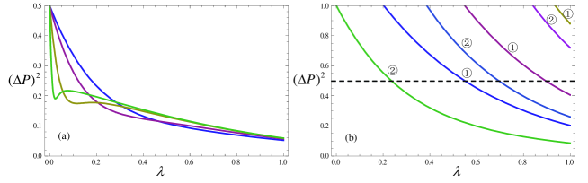
Figure 2: (Color online) The fluctuations variation of $(\Delta P)^{2}$ with $\lambda$ for several different parameters $m,n$ values: (a) $m=n=1,2,8,35$ from down to up; (b) (1) and (2) denote $m=0$ and $m=1$, respectively, and $n=2,5,12$ from down to up.

III.2 Distribution of photon number

In order to obtain the photon number distribution of the TPSSV, we begin with evaluating the overlap between two-mode number state $\left\langle n_{a},n_{b}\right|$ and $\left|\lambda,m,n\right\rangle.$ Using Eq.(1) and the un-normalized coherent state 30 ; 31 , $\left|z\right\rangle=\exp\left(za^{\dagger}\right)\left|0\right\rangle$, leading to $\left\langle n\right|=\frac{1}{\sqrt{n!}}\left.\frac{\partial^{n}}{\partial z^{\ast n}}\left\langle z\right|\right|_{z^{\ast}=0}$, it is easy to see that

$$\left\langle n_{a},n_{b}\right.\left|\lambda,m,n\right\rangle$$

$$=\text{sech}\lambda\left\langle n_{a},n_{b}\right|a^{m}b^{n}e^{a^{\dagger}b^{\dagger}\tanh\lambda}\left|00\right\rangle$$

$$=\frac{\left(m+n_{a}\right)!}{\sqrt{n_{a}!n_{b}!}}\text{sech}\lambda\tanh^{m+n_{a}}\lambda\delta_{m+n_{a},n+n_{b}}.$$ (24)

It is easy to follow that the photon number distribution of $|\left|\lambda,m,n\right\rangle$, i.e.,

$$P(n_{a},n_{b}) =N_{\lambda,m,n}^{-1}\left|\left\langle n_{a},n_{b}\right.\left|\lambda,m,n\right\rangle\right|^{2}$$

$$=\frac{\left[\left(m+n_{a}\right)!\text{sech}\lambda\tanh^{m+n_{a}}\lambda\delta_{m+n_{a},n+n_{b}}\right]^{2}}{n_{a}!n_{b}!m!n!\sinh^{2n}\lambda P_{m}^{(n-m,0)}(\cosh 2\lambda)}.$$ (25)

From Eq.(25) one can see that there exists a constrained condition, $m+n_{a}=n+n_{b},$ for the photon number distribution (see Fig. 3). In particular, when $m=n=0,$ Eq.(25) becomes

$$P(n_{a},n_{b})=\left\{\begin{array}[c]{cc}\text{sech}^{2}\lambda\tanh^{2n_{a}}\lambda,&n_{a}=n_{b}\\ 0,&n_{a}\neq n_{b}\end{array}\right.,$$ (26)

which is just the photon number distribution (PND) of two-mode squeezed vacuum state.

In Fig. 3, we plot the distribution $P(n_{a},n_{b})$ in the Fock space ($n_{a},n_{b}$) for some given $m,n$ values and squeezing parameter $\lambda$. From Fig. 3 it is found that the PND is constrained by $m+n_{a}=n+n_{b},$ resulting from the paired-present of photons in two-mode squeezed state. By subtracting photons, we have been able to move the peak from zero photons to nonzero photons (see Fig.3 (a) and (c)). The position of peak depends on how many photons are annihilated and how much the state is squeezed initially. In addition, for example, the PND mainly shifts to the bigger number states and becomes more “flat” and “wide” with the increasing parameter $\lambda$ (see Fig.3 (b) and (c)).

Figure 3: (Color online) Photon number distribution $P(n_{a},n_{b})$ in the Fock space ($n_{a},n_{b}$) for some given $m=n$ values: (a) $m=n=0,$ $\lambda=1$, (b) $m=n=1,$ $\lambda=0.5,$(c) $m=n=1,$ $\lambda=1,$(d) $m=2,n=5,$ $\lambda=1.$

III.3 Antibunching effect of the TPSSV

Next we will discuss the antibunching for the TPSSV. The criterion for the existence of antibunching in two-mode radiation is given by 33

$$R_{ab}\equiv\frac{\left\langle a^{\dagger 2}a^{2}\right\rangle+\left\langle b^{\dagger 2}b^{2}\right\rangle}{2\left\langle a^{\dagger}ab^{\dagger}b\right\rangle}-1<0.$$ (27)

In a similar way to Eq.(13) we have

$$\left\langle a^{\dagger 2}a^{2}\right\rangle=\left(m+1\right)\left(m+2\right)\frac{P_{m+2}^{(n-m-2,0)}(\tau)}{P_{m}^{(n-m,0)}(\tau)},$$ (28)

and

$$\left\langle b^{\dagger 2}b^{2}\right\rangle=\left(n+1\right)\left(n+2\right)\sinh^{4}\lambda\frac{P_{m}^{(n-m+2,0)}(\tau)}{P_{m}^{(n-m,0)}(\tau)},$$ (29)

For the state $|\left|\lambda,m,n\right\rangle$, substituting Eqs.(15), (28)and (29) into Eq.(27), we can recast $R_{ab}$ to

$$R_{ab}=\frac{\left(m+1\right)\left(m+2\right)P_{m+2}^{(n-m-2,0)}(\tau)+\left(n+1\right)\left(n+2\right)\sinh^{4}\lambda P_{m}^{(n-m+2,0)}(\tau)}{2\left(m+1\right)\left(n+1\right)\sinh^{2}\lambda P_{m+1}^{(n-m,0)}(\tau)}-1.$$ (30)

In particular, when $m=n=0$ (corresponding to two-mode squeezed vacuum state), Eq.(30) reduces to $R_{ab,m=n=0}=-\operatorname{sech}2\lambda<0,$ which indicates that there always exist antibunching effect for two-mode squeezed vacuum state. In addition, when $m=n,$ the TPSSV is always antibunching. However, for any parameter values $m,n(m\neq n)$, the case is not true. The $R_{ab}$ as a function of $\lambda$ and $m,n$ is plotted in Fig. 4. It is easy to see that, for a given $m$ the TPSSV presents the antibunching effect when the squeezing parameter $\lambda$ exceeds to a certain threshold value. For instance, when $m=0\$and $n=2$ then $R_{ab}=\frac{5-3\cosh 2\lambda}{6\left(1+2\cosh 2\lambda\right)}$csch${}^{2}\lambda$ may be less than zero with $\lambda>0.549$ about.

Figure 4: (Color online) The $R_{ab}$ as a function of $\lambda$ and $m,n$. (1) and (2) in Fig.4 (a) denote$m=0$ and $m=1$ respectively, and $n=2,3,12$ from down to up.

IV Wigner function of the TPSSV

The Wigner function (WF)25 ; 34 ; 35 is a powerful tool to investigate the nonclassicality of optical fields. Its partial negativity implies the highly nonclassical properties of quantum states and is often used to describe the decoherence of quantum states, e.g., the excited coherent state in both photon-loss and thermal channels 36 ; 37 , the single-photon subtracted squeezed vacuum (SPSSV) state in both amplitude decay and phase damping channels 2d , and so on 4 ; 10 ; 38 ; 39 ; 40 . In this section, we derive the analytical expression of WF for the TPSSV. For this purpose, we first recall that the Weyl ordered form of single-mode Wigner operator 41 ; 42 ; 43 ,

$$\Delta_{1}\left(\alpha\right)=\frac{1}{2}\genfrac{}{}{0.0pt}{}{\colon}{\colon}\delta\left(\alpha-a\right)\delta\left(\alpha^{\ast}-a^{{\dagger}}\right)\genfrac{}{}{0.0pt}{}{\colon}{\colon},$$ (31)

where $\alpha=\left(q_{1}+ip_{1}\right)/\sqrt{2}$ and the symbol $\genfrac{}{}{0.0pt}{}{\colon}{\colon}\genfrac{}{}{0.0pt}{}{\colon}{\colon}$ denotes Weyl ordering. The merit of Weyl ordering lies in the Weyl ordered operators’ invariance under similar transformations proved in Ref.41 , which means

$$S\genfrac{}{}{0.0pt}{}{:}{:}\left(\circ\circ\circ\right)\genfrac{}{}{0.0pt}{}{:}{:}S^{-1}=\genfrac{}{}{0.0pt}{}{:}{:}S\left(\circ\circ\circ\right)S^{-1}\genfrac{}{}{0.0pt}{}{:}{:},$$ (32)

as if the “fence” $\genfrac{}{}{0.0pt}{}{:}{:}\genfrac{}{}{0.0pt}{}{:}{:}$did not exist, so $S$ can pass through it.

Following this invariance and Eq.(3) we have

$$S_{2}^{{\dagger}}\left(\lambda\right)\Delta_{1}\left(\alpha\right)\Delta_{2}\left(\beta\right)S_{2}\left(\lambda\right)$$

$$=\frac{1}{4}S_{2}^{{\dagger}}\left(\lambda\right)\genfrac{}{}{0.0pt}{}{\colon}{\colon}\delta\left(\alpha-a\right)\delta\left(\alpha^{\ast}-a^{{\dagger}}\right)\delta\left(\beta-b\right)\delta\left(\beta^{\ast}-b^{{\dagger}}\right)\genfrac{}{}{0.0pt}{}{\colon}{\colon}S_{2}\left(\lambda\right)$$

$$=\frac{1}{4}\genfrac{}{}{0.0pt}{}{\colon}{\colon}\delta\left(\alpha-a\cosh\lambda-b^{\dagger}\sinh\lambda\right)\delta\left(\alpha^{\ast}-a^{\dagger}\cosh\lambda-b\sinh\lambda\right)$$

$$\delta\left(\beta-b\cosh\lambda-a^{\dagger}\sinh\lambda\right)\delta\left(\beta^{\ast}-b^{\dagger}\cosh\lambda-a\sinh\lambda\right)\genfrac{}{}{0.0pt}{}{\colon}{\colon}$$

$$=\frac{1}{4}\genfrac{}{}{0.0pt}{}{\colon}{\colon}\delta\left(\bar{\alpha}-a\right)\delta\left(\bar{\alpha}^{\ast}-a^{{\dagger}}\right)\delta\left(\bar{\beta}-b\right)\delta\left(\bar{\beta}^{\ast}-b^{{\dagger}}\right)\genfrac{}{}{0.0pt}{}{\colon}{\colon}$$

$$=\Delta_{1}\left(\bar{\alpha}\right)\Delta_{2}\left(\bar{\beta}\right),$$

where $\bar{\alpha}=\alpha\cosh\lambda-\beta^{\ast}\sinh\lambda,$ $\bar{\beta}=\beta\cosh\lambda-\alpha^{\ast}\sinh\lambda,$ and $\beta=\left(q_{2}+ip_{2}\right)/\sqrt{2}$. Thus employing the squeezed two-variable Hermite-excited vacuum state of the TPSSV in Eq.(5) and the coherent state representation of single-mode Wigner operator 44 ,

$$\Delta_{1}(\alpha)=e^{2\left|\alpha\right|^{2}}\int\frac{d^{2}z_{1}}{\pi^{2}}\left|z_{1}\right\rangle\left\langle-z_{1}\right|e^{-2(z_{1}\alpha^{\ast}-\alpha z_{1}^{\ast})},$$ (33)

where $\left|z_{1}\right\rangle=\exp\left(z_{1}a^{{\dagger}}-z_{1}^{\ast}a\right)\left|0\right\rangle$ is Glauber coherent state 30 ; 31 , we finally can obtain the explicit expression of WF for the TPSSV (see Appendix A),

$$W(\alpha,\beta) =\frac{1}{\pi^{2}}\frac{\sinh^{n+m}2\lambda}{2^{n+m}N_{\lambda,m,n}}e^{-2\left|\bar{\alpha}\right|^{2}-2\left|\bar{\beta}\right|^{2}}\sum_{l=0}^{m}\sum_{k=0}^{n}$$

$$\times\frac{\left[m!n!\right]^{2}\left(-\tanh\lambda\right)^{l+k}}{l!k!\left[\left(m-l\right)!\left(n-k\right)!\right]^{2}}\left|H_{m-l,n-k}\left(B,A\right)\right|^{2},$$ (34)

where we have set $A=-2i\bar{\alpha}\sqrt{\tanh\lambda},B=-2i\bar{\beta}\sqrt{\tanh\lambda}.$ Obviously, the WF $W(\alpha,\beta)$ in Eq.(34) is a real function and is non-Gaussian in phase space due to the presence of $H_{m-l,n-k}\left(B,A\right)$, as expected.

In particular, when $m=n=0,$ Eq.(34) reduces to $W(\alpha,\beta)=\frac{1}{\pi^{2}}e^{-2\left|\bar{\alpha}\right|^{2}-2\left|\bar{\beta}\right|^{2}}=\frac{1}{\pi^{2}}e^{2\left(\alpha^{\ast}\beta^{\ast}+\alpha\allowbreak\beta\right)\sinh 2\lambda-2\left(\alpha\alpha^{\ast}+\beta\beta^{\ast}\allowbreak\right)\cosh 2\lambda}$ corresponding to the WF of two-mode squeezed vacuum state; while for the case of $m=0$ and $n\neq 0,$ noticing $H_{0,n}\left(x,y\right)=y^{n}$ and $N_{\lambda,0,n}=n!\sinh^{2n}\lambda,$ Eq.(34) becomes

$$W(\alpha,\beta)=\frac{\left(-1\right)^{n}}{\pi^{2}}e^{-2\left|\bar{\alpha}\right|^{2}-2\left|\bar{\beta}\right|^{2}}L_{n}\left(4\left|\bar{\alpha}\right|^{2}\right),$$ (35)

where $L_{n}$ is $m$-order Laguerre polynomials and Eq.(35) is just the WF of the negative binomial state $S_{2}(\lambda)\left|n,0\right\rangle$ 28 . In Figs. 5-7, the phase space Wigner distributions are depicted for several different parameter values $m,n$, and $\lambda$. As an evidence of nonclassicality of the state, squeezing in one of quadratures is clear in the plots. In addition, there are some negative region of the WF in the phase space which is another indicator of the nonclassicality of the state. For the case of $m=0$ and $n=1,$ it is easily seen from (35) that at the center of the phase space ($\alpha=\beta=0$), the WF is always negative in phase space. Fig.5 shows that the negative region becomes more and visible as the increasement of photon number subtracted $m(=n)$, which may imply the nonclassicality of the state can be enhanced due to the augment of photon-subtraction number. For a given value $m$ and several different values $n$ ($\neq m$), the WF distributions are presented in Fig.7, from which it is interseting to notice that there are around $\left|m-n\right|$ wave valleys and $\left|m-n\right|+1$ wave peaks.

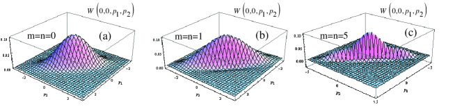
Figure 5: (Color online) The Wigner function W($\alpha,\beta$) in phase space ($0,0,p_{1},p_{2}$) for several different parameter values $m=n$ with $\lambda=0.5.$ (a) m=n=0; (b) m=n=1 and (c) m=n=5.

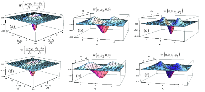
Figure 6: (Color online) The Wigner function W($\alpha,\beta$) in three different phase spaces for $m=0,n=1$ with $\lambda=0.3$ (first row) and $\lambda=0.5\$(second low).

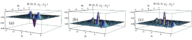
Figure 7: (Color online) The Wigner function W($\alpha,\beta$) in phase space ($0,0,p_{1},p_{2}$) for several parameter values $m,n$ with $\lambda=0.5.$ (a) m1,=n=2; (b) m=1,n=3 and (c) m=1,n=5.

V Decoherence of TPSSV in thermal environments

In this section, we next consider how this state evolves at the presence of thermal environment.

V.1 Model

When the TPSSV evolves in the thermal channel, the evolution of the density matrix can be described by the following master equation in the interaction picture45

$$\frac{d}{dt}\rho\left(t\right)=\left(L_{1}+L_{2}\right)\rho\left(t\right),$$ (36)

where

$$L_{i}\rho =\kappa\left(\bar{n}+1\right)\left(2a_{i}\rho a_{i}^{{\dagger}}-a_{i}^{{\dagger}}a_{i}\rho-\rho a_{i}^{{\dagger}}a_{i}\right)$$

$$+\kappa\bar{n}\left(2a_{i}^{{\dagger}}\rho a_{i}-a_{i}a_{i}^{{\dagger}}\rho-\rho a_{i}a_{i}^{{\dagger}}\right),\text{ }\left(a_{1}=a,a_{2}=b\right),$$ (37)

and $\kappa$ represents the dissipative coefficient and $\bar{n}$ denotes the average thermal photon number of the environment. When $\bar{n}=0,$ Eq.(36) reduces to the master equation (ME) describing the photon-loss channel. The two thermal modes are assumed to have the same average energy and coupled with the channel in the same strength and have the same average thermal photon number $\bar{n}$. This assumption is reasonable as the two-mode of squeezed state are in the same frequency and temperature of the environment is normally the same 46 ; 47 . By introducing two entangled state representations and using the technique of integration within an ordered product (IWOP) of operators, we can obtain the infinite operator-sum expression of density matrix in Eq.(36) (see Appendix B):

$$\rho\left(t\right)=\sum_{i,j,r,s=0}^{\infty}M_{i,j,r,s}\rho_{0}M_{i,j,r,s}^{{\dagger}},$$ (38)

where $\rho_{0}$ denotes the density matrix at initial time, $M_{i,j,r,s}$ and $M_{i,j,r,s}^{{\dagger}}$ are Hermite conjugated operators (Kraus operator) with each other,

$$M_{i,j,r,s}=\frac{1}{\bar{n}T+1}\sqrt{\frac{\left(T_{1}\right)^{r+s}\left(T_{3}\right)^{i+j}}{r!s!i!j!}}a^{\dagger r}b^{\dagger s}e^{\left(a^{\dagger}a+b^{\dagger}b\right)\ln T_{2}}a^{i}b^{j},$$ (39)

and we have set $T=1-e^{-2\kappa t}$, as well as

$$T_{1}=\frac{\bar{n}T}{\bar{n}T+1},T_{2}=\frac{e^{-\kappa t}}{\bar{n}T+1},T_{3}=\frac{\left(\bar{n}+1\right)T}{\bar{n}T+1}.$$ (40)

It is not difficult to prove the $M_{i,j,r,s}$ obeys the normalization condition $\sum_{i,j,r,s=0}^{\infty}M_{i,j,r,s}^{{\dagger}}M_{i,j,r,s}=1$ by using the IWOP technique.

V.2 Evolution of Wigner function

By using the thermal field dynamics theory 48 ; 49 and thermal entangled state representation, the time evolution of Wigner function at time $t$ to be given by the convolution of the Wigner function at initial time and those of two single-mode thermal state (see Appendix C), i.e.,

$$W\left(\alpha,\beta,t\right)=\frac{4}{\left(2\bar{n}+1\right)^{2}T^{2}}\int\frac{d^{2}\zeta d^{2}\eta}{\pi^{2}}W\left(\zeta,\eta,0\right)e^{-2\frac{\left|\alpha-\zeta e^{-\kappa t}\right|^{2}+\left|\beta-\eta e^{-\kappa t}\right|^{2}}{\left(2\bar{n}+1\right)T}}.$$ (41)

Eq.(41) is just the evolution formula of Wigner function of two-mode quantum state in thermal channel. Thus the WF at any time can be obtained by performing the integration when the initial WF is known.

In a similar way to deriving Eq.(34), substituting Eq.(34) into Eq.(41) and using the generating function of two-variable Hermite polynomials (A2), we finally obtain

$$W\left(\alpha,\beta,t\right) =\frac{N_{\lambda,m,n}^{-1}\left(E\sinh 2\lambda\right)^{m+n}}{\pi^{2}2^{n+m}\left(2\bar{n}+1\right)^{2}T^{2}D}e^{-\frac{\left|\alpha-\beta^{\ast}\right|^{2}}{e^{-2\lambda-2\kappa t}+\left(2\bar{n}+1\right)T}-\frac{\left|\alpha+\beta^{\ast}\right|^{2}}{e^{2\lambda-2\kappa t}+\left(2\bar{n}+1\right)T}}$$

$$\times\sum_{l=0}^{n}\sum_{k=0}^{m}\frac{\left[m!n!\right]^{2}\left(-\frac{F}{E}\tanh\lambda\right)^{l+k}}{l!k!\left[\left(m-k\right)!\left(n-l\right)!\right]^{2}}\left|H_{m-k,n-l}\left(G/\sqrt{E},K/\sqrt{E}\right)\right|^{2},$$ (42)

where we have set

$$C =\frac{e^{-2\kappa t}}{\left(2\bar{n}+1\right)T},\text{ }D=\left(1+Ce^{-2\lambda}\right)\left(1+Ce^{2\lambda}\right),$$

$$E =\allowbreak\frac{e^{4\kappa t}}{D}\left(2\bar{n}T+1\right)^{2}C^{2},\text{ }F=\frac{C^{2}-1}{D},$$

$$G =\frac{Ce^{\kappa t}}{D}\left(\bar{B}+B^{\ast}\allowbreak C\right),\text{ }\bar{B}=\allowbreak i2\sqrt{\tanh\lambda}\left(\beta^{\ast}\cosh\lambda+\alpha\allowbreak\sinh\lambda\right),$$

$$K =\frac{Ce^{\kappa t}}{D}\left(\bar{A}+A^{\ast}C\right),\text{ }\bar{A}=i2\sqrt{\tanh\lambda}\left(\alpha^{\ast}\cosh\lambda+\beta\sinh\lambda\right).$$ (43)

Eq.(42) is just the analytical expression of WF for the TPSSV in thermal channel. It is obvious that the WF loss its Gaussian property due to the presence of two-variable Hermite polynomials.

In particular, at the initial time ($t=0$), noting $E\rightarrow 1$, $\left(2\bar{n}+1\right)^{2}T^{2}D\rightarrow 1$, $\frac{F}{E}\rightarrow 1$ and $\frac{C^{2}}{D}\rightarrow 1,$ $\frac{C}{D}\rightarrow 0$ as well as $K\rightarrow A^{\ast}$, $G\rightarrow B^{\ast}$, Eq.(42) just dose reduce to Eq.(34), i.e., the WF of the TPSSV. On the other hand, when $\kappa t\rightarrow\infty,$ noticing that $C\rightarrow 0,D\rightarrow 1,E\rightarrow 1,F\rightarrow-1,$ and $G/\sqrt{E}\rightarrow 0,K/\sqrt{E}\rightarrow 0,$ as well as $H_{m,n}\left(0,0\right)=\left(-1\right)^{m}m!\delta_{m,n},$ as well as the definition of Jacobi polynomials in Eq.(9), then Eq.(42) becomes

$$W\left(\alpha,\beta,\infty\right)=\frac{1}{\pi^{2}\left(2\bar{n}+1\right)^{2}}e^{-\frac{2}{2\bar{n}+1}(\left|\alpha\right|^{2}+\left|\beta\right|^{2})},$$ (44)

which is independent of photon-subtraction number $m$ and $n$ and corresponds to the product of two thermal states with mean thermal photon number $\bar{n}$. This implies that the two-mode system reduces to two-mode thermal state after a long time interaction with the environment. Eq.(44) denotes a Gaussian distribution. Thus the thermal noise causes the absence of the partial negative of the WF if the decay time $\kappa t$ exceeds a threshold value. In addition, for the case of $m=n=0$, corresponding to the case of two-mode squeezed vacuum, Eq.(42) just becomes

$$W_{m=n=0}\left(\alpha,\beta,t\right)=\mathfrak{N}^{-1}e^{-\frac{\mathfrak{E}}{\mathfrak{D}}\left(\left|\alpha\right|^{2}+\left|\beta\right|^{2}\right)+\frac{\mathfrak{F}}{\mathfrak{D}}\left(\alpha\beta+\alpha^{\ast}\beta^{\ast}\right)},$$ (45)

where $\mathfrak{N}=\pi^{2}\left(2\bar{n}+1\right)^{2}T^{2}D$ is the normalization factor, $\mathfrak{D}=\left(2\bar{n}+1\right)^{2}T^{2}D,$ $\mathfrak{E}=2\left(2\bar{n}+1\right)T+e^{-2\kappa t}\cosh 2\lambda,$ and $\mathfrak{F}=2e^{-2\kappa t}\sinh 2\lambda$. Eq.(45) is just the result in Eq.(14) of Ref. 47 .

In Fig.8, the WFs of the TPSSV for ($m=0,n=1$) are depicted in phase space with $\lambda=0.3$ and $\bar{n}=1$ for several different $\kappa t.$ It is easy to see that the negative region of WF gradually disappears as the time $\kappa t$ increases. Actually, from Eq.(43) one can see that $D>0$ and $E>0$, so when $F<0$ leading to the following condition:

$$\kappa t>\kappa t_{c}\equiv\frac{1}{2}\ln\frac{2\bar{n}+2}{2\bar{n}+1},$$ (46)

we know that the WF of TPSSV has no chance to be negative in the whole phase space when $\kappa t\$exceeds a threshold value $\kappa t_{c}$. Here we should point out that the effective threshold value of the decay time corresponding to the transition of the WF from partial negative to fully positive definite is dependent of $m\$and $n.$ When $\kappa t=\kappa t_{c},$ it then follows from Eq.(42) that

$$W\left(\alpha,\beta,t_{c}\right) =\frac{\tanh^{m+n}\lambda\operatorname{sech}^{2}\lambda}{4\pi^{2}N_{m,n,\lambda}e^{-4\kappa t_{c}}}e^{-e^{2\kappa t_{c}}\left[\left|\alpha\right|^{2}+\left|\beta\right|^{2}-\left(\alpha^{\ast}\beta^{\ast}+\alpha\beta\right)\tanh\lambda\right]}$$

$$\times\left|H_{m,n}\left(i\sqrt{\tanh\lambda}\beta^{\ast}e^{\kappa t_{c}},\allowbreak i\sqrt{\tanh\lambda}\alpha^{\ast}e^{\kappa t_{c}}\right)\right|^{2},$$ (47)

which is an Hermite-Gaussian function and positive definite, as expected.

In Figs. 9 and 10, we have presented the time-evolution of WF in phase space for different $\bar{n}$ and $\lambda,$ respectively. One can see clearly that the partial negativity of WF decreases gradually as $\bar{n}$ (or $\lambda$) increases for a given time. This case is true for a given $\bar{n}$ (or $\kappa t$) as the increasement of $\kappa t$ (or $\bar{n}$). The squeezing effect in one of quadratures is shown in Fig.10. In principle, by using the explicit expression of WF in Eq.(42), we can draw its distributions in phase space. For the case of $m=0,n=2$, there are two negative regions of WF, which is different from the case of $m=0,n=1$ (see Fig.11). The absolute value of the negative minimum of the WF decreases as $\kappa t$ increases, which leads to the full absence of partial negative region.

Figure 8: (Color online) The time evolution of WF $\left(m=0,n=1\right)$ at $\left(q_{1},q_{2},0,0\right)$ phase space for $\bar{n}=1,\lambda=0.3.$(a) $\kappa t=0.05,$(b) $\kappa t=0.1,$(c) $\kappa t=0.12,$(d) $\kappa t=0.2.$

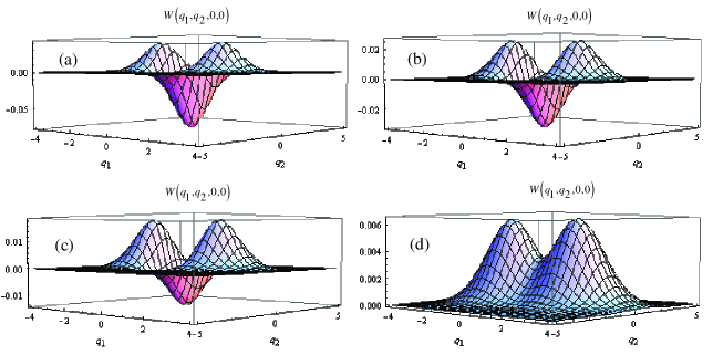
Figure 9: (Color online) The time evolution of WF $\left(m=0,n=1\right)$ in $\left(q_{1},q_{2},0,0\right)$ phase space for $\lambda=0.3\$and $\kappa t=0.05\$with (a) $\bar{n}=0,$(b) $\bar{n}=1,$(c) $\bar{n}=2,$(d) $\bar{n}=7.$

Figure 10: (Color online) The time evolution of WF $\left(m=0,n=1\right)$ in $\left(q_{1},q_{2},0,0\right)$ phase space for $\bar{n}=1,$and $\kappa t=0.05\$with (a) $\lambda=0.03,$(b) $\lambda=0.5,$(c) $\lambda=0.8,$(d) $\lambda=1.2.$

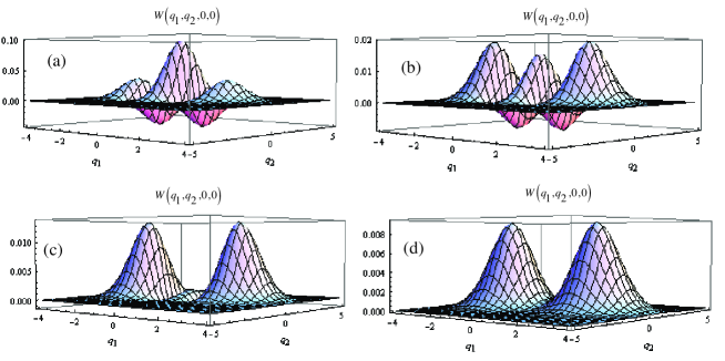
Figure 11: (Color online) The time evolution of WF for $m=0,n=2$ in $\left(q_{1},q_{2},0,0\right)$ phase space with (a) $\kappa t=0,$(b) $\kappa t=0.05,$(c) $\kappa t=0.1,$(d) $\kappa t=0.2.$

VI Conclusions

In summary, we have investigated the statistical properties of two-mode photon-subtracted squeezed vacuum state (TPSSV) and its decoherence in thermal channelwith average thermal photon number $\bar{n}$ and dissipative coefficient $\kappa$. For arbitrary number TPSSV, we have for the first time calculated the normalization factor, which turns out to be a Jacobi polynomial of the squeezing parameter $\lambda$, a remarkable result. We also show that the TPSSV can be treated as a squeezed two-variable Hermite polynomial excitation vacuum. Based on Jacobi polynomials’ behavior the statistical properties of the field, such as photon number distribution, squeezing properties, cross-correlation function and antibunching, are also derived analytically. Especially, the nonclassicality of TPSSV is discussed in terms of the negativity of WF after deriving the explicit expression of WF. Then the decoherence of TPSSV in thermal channel is also demonstrated according to the compact expression for the WF. The threshold value of the decay time corresponding to the transition of the WF from partial negative to completely positive is presented. It is found that the WF has no chance to present negative value for all parameters $\lambda$ and any photon-subtraction number ($m,n$) if $\kappa t>\frac{1}{2}\ln\frac{2\bar{n}+2}{2\bar{n}+1}\$for TPSSV. The technique of integration within an ordered product of operators brings convenience in our derivation.

Acknowledgments Work supported by the the National Natural Science Foundation of China under Grant Nos.10775097 and 10874174.

Appendix A: Deriviation of Wigner function Eq.(34) of TPSSV

The definite of the WF of two-mode quantum state $\left|\Psi\right\rangle$ is given by $W(\alpha,\beta)=\left\langle\Psi\right|\Delta_{1}\left(\alpha\right)\Delta_{2}\left(\beta\right)\left|\Psi\right\rangle$, thus by uisng Eqs.(5), and (33) the WF of TPSSV can be calculated as

$$W(\alpha,\beta) =\left\langle\lambda,m,n\right||\Delta_{1}\left(\alpha\right)\Delta_{2}\left(\beta\right)|\left|\lambda,m,n\right\rangle$$

$$=\frac{\sinh^{n+m}2\lambda}{2^{n+m}N_{\lambda,m,n}}\left\langle 00\right|H_{m,n}\left(-i\sqrt{\tanh\lambda}b,-i\sqrt{\tanh\lambda}a\right)\Delta_{1}\left(\bar{\alpha}\right)$$

$$\otimes\Delta_{2}\left(\bar{\beta}\right)H_{m,n}\left(i\sqrt{\tanh\lambda}b^{\dagger},i\sqrt{\tanh\lambda}a^{\dagger}\right)\left|00\right\rangle$$

$$=\frac{\sinh^{n+m}2\lambda}{2^{n+m}N_{\lambda,m,n}}e^{2\left|\bar{\alpha}\right|^{2}+2\left|\bar{\beta}\right|^{2}}\int\frac{d^{2}z_{1}d^{2}z_{2}}{\pi^{4}}e^{-\left|z_{1}\right|^{2}-\left|z_{2}\right|^{2}-2(z_{1}\bar{\alpha}^{\ast}-\bar{\alpha}z_{1}^{\ast})-2(z_{2}\bar{\beta}^{\ast}-\bar{\beta}z_{2}^{\ast})}$$

$$\times H_{m,n}\left(-i\sqrt{\tanh\lambda}z_{2},-i\sqrt{\tanh\lambda}z_{1}\right)H_{m,n}\left(-i\sqrt{\tanh\lambda}z_{2}^{\ast},-i\sqrt{\tanh\lambda}z_{1}^{\ast}\right).$$ (A1)

Further noticing the generating function of two variables Hermitian polynomials,

$$H_{m,n}\left(\epsilon,\varepsilon\right)=\frac{\partial^{m+n}}{\partial t^{m}\partial t^{\prime n}}\left.\exp\left[-tt^{\prime}+\epsilon t+\varepsilon t^{\prime}\right]\right|_{t=t^{\prime}=0},$$ (A2)

Eq.(A1) can be further rewritten as

$$W(\alpha,\beta) =\frac{\sinh^{n+m}2\lambda}{2^{n+m}N_{\lambda,m,n}}e^{2\left|\bar{\alpha}\right|^{2}+2\left|\bar{\beta}\right|^{2}}\frac{\partial^{m+n}}{\partial t^{m}\partial\tau^{n}}\frac{\partial^{m+n}}{\partial t^{\prime m}\partial\tau^{\prime n}}e^{-t\tau-t^{\prime}\tau^{\prime}}$$

$$\times\int\frac{d^{2}z_{1}}{\pi^{2}}\left.e^{-\left|z_{1}\right|^{2}+\left(-2\bar{\alpha}^{\ast}-i\sqrt{\tanh\lambda}\tau\right)z_{1}+\left(2\bar{\alpha}-i\sqrt{\tanh\lambda}\tau^{\prime}\right)z_{1}^{\ast}}\right|_{t=\tau=0}$$

$$\times\int\frac{d^{2}z_{2}}{\pi^{2}}\left.e^{-\left|z_{2}\right|^{2}+\left(-2\bar{\beta}^{\ast}-i\sqrt{\tanh\lambda}t\right)z_{2}+\left(2\bar{\beta}-i\sqrt{\tanh\lambda}t^{\prime}\right)z_{2}^{\ast}}\right|_{t^{\prime}=\tau^{\prime}=0}$$

$$=\frac{\sinh^{n+m}2\lambda}{2^{n+m}N_{\lambda,m,n}}e^{-2\left|\bar{\alpha}\right|^{2}-2\left|\bar{\beta}\right|^{2}}\frac{\partial^{m+n}}{\partial t^{m}\partial\tau^{n}}\frac{\partial^{m+n}}{\partial t^{\prime m}\partial\tau^{\prime n}}$$

$$\times\left.e^{-t\tau-t^{\prime}\tau^{\prime}+A^{\ast}\tau\prime+B^{\ast}t^{\prime}\allowbreak+A\tau+Bt-\left(tt^{\prime}+\tau\tau^{\prime}\right)\tanh\lambda}\right|_{t=\tau=t^{\prime}=\tau^{\prime}=0},$$ (A3)

where we have set

$$B=-2i\bar{\beta}\sqrt{\tanh\lambda},A=-2i\bar{\alpha}\sqrt{\tanh\lambda},$$ (A4)

and have used the following integration formula

$$\int\frac{d^{2}z}{\pi}e^{\zeta\left|z\right|^{2}+\xi z+\eta z^{\ast}}=-\frac{1}{\zeta}e^{-\frac{\xi\eta}{\zeta}},\text{Re}\left(\zeta\right)<0.$$ (A5)

Expanding the exponential term $\exp\left[-\left(tt^{\prime}+\tau\tau^{\prime}\right)\tanh\lambda\right],$ and using Eq.(A2), we have

$$W(\alpha,\beta) =\frac{\sinh^{n+m}2\lambda}{2^{n+m}N_{\lambda,m,n}}e^{-2\left|\bar{\alpha}\right|^{2}-2\left|\bar{\beta}\right|^{2}}\sum_{l=0}^{\infty}\sum_{k=0}^{\infty}\frac{\left(-\tanh\lambda\right)^{l+k}}{l!k!}$$

$$\allowbreak\times\frac{\partial^{l+k}}{\partial B^{l}\partial A^{k}}\frac{\partial^{l+k}}{\partial B^{\ast l}\partial A^{\ast k}}\frac{\partial^{2m}}{\partial t^{m}\partial\tau^{n}}$$

$$\times\left.\frac{\partial^{2n}}{\partial t^{\prime m}\partial\tau^{\prime n}}e^{-t\tau+A\tau+Bt-t^{\prime}\tau^{\prime}+A^{\ast}\tau\prime+B^{\ast}t^{\prime}\allowbreak}\right|_{t=\tau=t^{\prime}=\tau^{\prime}=0}$$

$$=\frac{\sinh^{n+m}2\lambda}{2^{n+m}N_{\lambda,m,n}}e^{-2\left|\bar{\alpha}\right|^{2}-2\left|\bar{\beta}\right|^{2}}\sum_{l=0}^{\infty}\sum_{k=0}^{\infty}\frac{\left(-\tanh\lambda\right)^{l+k}}{l!k!}$$

$$\times\frac{\partial^{l+k}}{\partial B^{l}\partial A^{k}}\frac{\partial^{l+k}}{\partial B^{\ast l}\partial A^{\ast k}}H_{m,n}\left(B,A\right)H_{m,n}\left(B^{\ast},A^{\ast}\right).$$ (A6)

Noticing the well-known differential relations of $H_{m,n}\left(\epsilon,\varepsilon\right),$

$$\frac{\partial^{l+k}}{\partial\epsilon^{l}\partial\varepsilon^{k}}H_{m,n}\left(\epsilon,\varepsilon\right)=\frac{m!n!H_{m-l,n-k}\left(\epsilon,\varepsilon\right)}{\left(m-l\right)!\left(n-k\right)!},$$ (A7)

we can further recast Eq.(A6) to Eq.(34).

Appendix B: Derivation of solution of Eq.(36)

To solve the ME in Eq.(36), we first introduce two entangled state representations 49a :

$$\left|\eta_{a}\right\rangle =\exp\left[-\frac{1}{2}|\eta_{a}|^{2}+\eta_{a}a^{\dagger}-\eta_{a}^{\ast}\tilde{a}^{\dagger}+a^{\dagger}\tilde{a}^{\dagger}\right]\left|0\tilde{0}\right\rangle,$$ (B1)

$$\left|\eta_{b}\right\rangle =\exp\left[-\frac{1}{2}|\eta_{b}|^{2}+\eta_{b}b^{\dagger}-\eta_{b}^{\ast}\tilde{b}^{\dagger}+b^{\dagger}\tilde{b}^{\dagger}\right]\left|0\tilde{0}\right\rangle,$$ (B2)

which satisfy the following eigenvector equations, for instance,

$$\begin{array}[c]{c}(a-\tilde{a}^{\dagger})\left|\eta_{a}\right\rangle=\eta_{a}\left|\eta_{a}\right\rangle,\;(a^{\dagger}-\tilde{a})\left|\eta_{a}\right\rangle=\eta_{a}^{\ast}\left|\eta_{a}\right\rangle,\\ \left\langle\eta_{a}\right|(a^{\dagger}-\tilde{a})=\eta_{a}^{\ast}\left\langle\eta_{a}\right|,\ \left\langle\eta_{a}\right|(a-\tilde{a}^{\dagger})=\eta_{a}\left\langle\eta_{a}\right|.\end{array}$$ (B3)

which imply operators $(a-\tilde{a}^{\dagger})$ and $(a^{\dagger}-\tilde{a})$ can be replaced by number $\eta_{a}$ and$\ \eta_{a}^{\ast},$ $\left[(a-\tilde{a}^{\dagger}),(a^{\dagger}-\tilde{a})\right]=0.$ Operating two-side of Eq.(36) on the vector $\left|I_{a},I_{b}\right\rangle\equiv\left|\eta_{a}=0\right\rangle\otimes\left|\eta_{b}=0\right\rangle$, (denote $\left|\rho\left(t\right)\right\rangle\equiv\rho\left(t\right)\left|I_{a},I_{b}\right\rangle),$ and noticing the corresponding relation:

$$\begin{array}[c]{c}a\left|I_{a},I_{b}\right\rangle=\tilde{a}^{\dagger}\left|I_{a},I_{b}\right\rangle,\text{ }a^{\dagger}\left|I_{a},I_{b}\right\rangle=\tilde{a}\left|I_{a},I_{b}\right\rangle,\\ b\left|I_{a},I_{b}\right\rangle=\tilde{b}^{\dagger}\left|I_{a},I_{b}\right\rangle,\text{ }b^{\dagger}\left|I_{a},I_{b}\right\rangle=\tilde{b}\left|I_{a},I_{b}\right\rangle,\end{array}$$ (B4)

we can put Eq.(36) into the following form:

$$\frac{d}{dt}\left|\rho\left(t\right)\right\rangle =\left[\kappa\left(\bar{n}+1\right)\left(2a\tilde{a}-a^{{\dagger}}a-\tilde{a}^{\dagger}\tilde{a}\right)+\kappa\bar{n}\left(2a^{{\dagger}}\tilde{a}^{\dagger}-aa^{{\dagger}}-\tilde{a}\tilde{a}^{{\dagger}}\right)\right.$$

$$\left.+\kappa\left(\bar{n}+1\right)\left(2b\tilde{b}-b^{{\dagger}}b-\tilde{b}^{{\dagger}}\tilde{b}\right)+\kappa\bar{n}\left(2b^{{\dagger}}\tilde{b}^{{\dagger}}-bb^{{\dagger}}-\tilde{b}\tilde{b}^{{\dagger}}\right)\right]\left|\rho\left(t\right)\right\rangle.$$ (B5)

It’s formal solution is given by

$$\left|\rho\left(t\right)\right\rangle =\exp\left[\kappa t\left(\bar{n}+1\right)\left(2a\tilde{a}-a^{{\dagger}}a-\tilde{a}^{\dagger}\tilde{a}\right)+\kappa t\bar{n}\left(2a^{{\dagger}}\tilde{a}^{\dagger}-aa^{{\dagger}}-\tilde{a}\tilde{a}^{{\dagger}}\right)\right.$$

$$\left.+\kappa t\left(\bar{n}+1\right)\left(2b\tilde{b}-b^{{\dagger}}b-\tilde{b}^{{\dagger}}\tilde{b}\right)+\kappa t\bar{n}\left(2b^{{\dagger}}\tilde{b}^{{\dagger}}-bb^{{\dagger}}-\tilde{b}\tilde{b}^{{\dagger}}\right)\right]\left|\rho_{0}\right\rangle,$$ (B6)

where $\left|\rho_{0}\right\rangle\equiv\rho_{0}\left|I_{a},I_{b}\right\rangle$. In order to solve Eq.(B6), noticing that, for example,

$$2a\tilde{a}-a^{{\dagger}}a-\tilde{a}^{\dagger}\tilde{a}=-\left(a^{{\dagger}}-\tilde{a}\right)\left(a-\tilde{a}^{{\dagger}}\right)+\tilde{a}a-\tilde{a}^{\dagger}a^{{\dagger}},$$ (B7)

we have

$$\left|\rho\left(t\right)\right\rangle =\exp\left[\left(a\tilde{a}-\tilde{a}^{\dagger}a^{\dagger}+1\right)\kappa t\right]$$

$$\times\exp\left[\frac{2\bar{n}+1}{2}\left(1-e^{2\kappa t}\right)\left(a^{\dagger}-\tilde{a}\right)\left(a-\tilde{a}^{\dagger}\right)\right]$$

$$\times\exp\left[\left(b\tilde{b}-\tilde{b}^{\dagger}b^{\dagger}+1\right)\kappa t\right]$$

$$\times\exp\left[\frac{2\bar{n}+1}{2}\left(1-e^{2\kappa t}\right)\left(b^{\dagger}-\tilde{b}\right)\left(b-\tilde{b}^{\dagger}\right)\right]\left|\rho_{0}\right\rangle,$$ (B8)

where we have used the identity operator, $\exp[\lambda(A+\sigma B)]=e^{\lambda A}\exp[\sigma B(1-e^{-\lambda\tau})/\tau]$ valid for $[A,B]=\tau B.$

Thus the element of $\rho\left(t\right)$ between $\left\langle\eta_{a},\eta_{b}\right|$ and $\left|I_{a},I_{b}\right\rangle$ is

$$\left\langle\eta_{a},\eta_{b}\right|\left.\rho\left(t\right)\right\rangle=\exp\left[-\frac{2\bar{n}+1}{2}T|\left(\eta_{a}|^{2}+|\eta_{b}|^{2}\right)\right]\left\langle\eta_{a}e^{-\kappa t},\eta_{b}e^{-\kappa t}\right|\left.\rho_{0}\right\rangle,$$ (B9)

from which one can see clearly the attenuation due to the presence of environment.

Further, using the completeness relation of $\left|\eta_{a},\eta_{b}\right\rangle$, $\int\frac{d^{2}\eta_{a}d^{2}\eta_{b}}{\pi^{2}}\left|\eta_{a},\eta_{b}\right\rangle\left\langle\eta_{a},\eta_{b}\right|=1$ and the IWOP technique 50 ; 51 , we see

$$\left|\rho\left(t\right)\right\rangle =\int\frac{d^{2}\eta_{a}d^{2}\eta_{b}}{\pi^{2}}\left|\eta_{a},\eta_{b}\right\rangle\left\langle\eta_{a},\eta_{b}\right|\left.\rho\left(t\right)\right\rangle$$

$$=\frac{1}{\left(\bar{n}T+1\right)^{2}}\exp\left[T_{1}\left(a^{\dagger}\tilde{a}^{\dagger}+b^{\dagger}\tilde{b}^{\dagger}\right)\right]$$

$$\times\exp\left[\left(a^{\dagger}a+b^{\dagger}b+\tilde{a}^{\dagger}\tilde{a}+\tilde{b}^{\dagger}\tilde{b}\right)\ln T_{2}\right]$$

$$\times\exp\left[T_{3}\left(a\tilde{a}+b\tilde{b}\right)\right]\rho_{0}\left|I_{a},I_{b}\right\rangle,$$ (B10)

where $T_{1},T_{2}$ and $T_{3}$ are defined in Eq.(40). Noticing Eq.(B4), we can reform Eq.(B10) as $\rho\left(t\right)=\sum_{i,j,r,s=0}^{\infty}M_{i,j,r,s}\rho_{0}M_{i,j,r,s}^{{\dagger}},$where $M_{i,j,r,s}$ and $M_{i,j,r,s}^{{\dagger}}$ are defined in Eq.(39).

Appendix C: Deriviation of Eq.(41) by using thermo field dynamics and entangled state representation

In this appendix, we shall derive the evolution formula of WF, i.e., the relation between the any time WF and the initial time WF. According to the definition of WF of density operator $\rho$: $W\left(\alpha\right)=\mathtt{Tr}\left[\Delta\left(\alpha\right)\rho\right]$, where $\Delta\left(\alpha\right)$ is the single-mode Wigner operator, $\Delta\left(\alpha\right)=\frac{1}{\pi}D\left(2\alpha\right)\left(-1\right)^{a^{{\dagger}}a}$. By using $\left\langle\tilde{n}\right.\left|\tilde{m}\right\rangle=\delta_{m,n}$ we can reform $W\left(\alpha\right)$ as 52

$$W\left(\alpha\right)=\sum_{m,n}^{\infty}\left\langle n,\tilde{n}\right|\Delta\left(\alpha\right)\rho\left|m,\tilde{m}\right\rangle=\frac{1}{\pi}\left\langle\xi_{=2\alpha}\right|\left.\rho\right\rangle,$$ (C1)

where $\left\langle\xi\right|$ is the conjugate state of $\left\langle\eta\right|$, whose overlap is $\left\langle\eta\right|\left.\xi\right\rangle=\frac{1}{2}\exp\left[\frac{1}{2}\left(\xi\eta^{\ast}-\xi^{\ast}\eta\right)\right],$a Fourier transformation kernel. In a similar way, thus for two-mode quantum system, the WF is given by

$$W\left(\alpha,\beta\right)=\mathtt{Tr}\left[\Delta_{a}\left(\alpha\right)\Delta_{b}\left(\beta\right)\rho\right]=\frac{1}{\pi^{2}}\left\langle\xi_{a=2\alpha},\xi_{b=2\beta}\right|\left.\rho\right\rangle.$$ (C2)

Employing the above overlap relation, Eq.(C2) can be recast into the following form:

$$W\left(\alpha,\beta,t\right)=\int\frac{d^{2}\eta_{a}d^{2}\eta_{b}}{4\pi^{4}}e^{\alpha^{\ast}\eta_{a}-\alpha\eta_{a}^{\ast}+\beta^{\ast}\eta_{b}-\beta\eta_{b}^{\ast}}\left\langle\eta_{a},\eta_{b}\right|\left.\rho\left(t\right)\right\rangle.$$ (C3)

Then substituting Eq.(B9) into Eq.(C3) and using the completeness of $\left\langle\xi\right|$, $\int\frac{d^{2}\xi}{\pi}\left|\xi\right\rangle\left\langle\xi\right|=1,$ we have

$$W\left(\alpha,\beta,t\right) =\int\frac{d^{2}\eta_{a}d^{2}\eta_{b}}{4\pi^{4}}e^{-\frac{2\bar{n}+1}{2}T|\left(\eta_{a}|^{2}+|\eta_{b}|^{2}\right)}$$

$$\times e^{\alpha^{\ast}\eta_{a}-\alpha\eta_{a}^{\ast}+\beta^{\ast}\eta_{b}-\beta\eta_{b}^{\ast}}\left\langle\eta_{a}e^{-\kappa t},\eta_{b}e^{-\kappa t}\right|\left.\rho_{0}\right\rangle$$

$$=\int\frac{d^{2}\xi_{a}d^{2}\xi_{b}}{\pi^{2}}W\left(\zeta,\eta,0\right)\int\frac{d^{2}\eta_{a}d^{2}\eta_{b}}{4\pi^{2}}e^{-\frac{2\bar{n}+1}{2}T|\left(\eta_{a}|^{2}+|\eta_{b}|^{2}\right)}$$

$$\times e^{\alpha^{\ast}\eta_{a}-\alpha\eta_{a}^{\ast}+\beta^{\ast}\eta_{b}-\beta\eta_{b}^{\ast}}\left\langle\eta_{a}e^{-\kappa t},\eta_{b}e^{-\kappa t}\right|\left.\xi_{a=2\zeta},\xi_{b=2\eta}\right\rangle.$$ (C4)

Performing the integration in Eq.(C4) over $d^{2}\eta_{a}d^{2}\eta_{b}$ then we can obtain Eq.(41).

Making variables replacement, $\frac{\alpha-\zeta e^{-\kappa t}}{\sqrt{T}}\rightarrow\zeta,$ $\frac{\beta-\eta e^{-\kappa t}}{\sqrt{T}}\rightarrow\eta,$ Eq.(41) can be reformed as

$$W\left(\alpha,\beta,t\right) =4e^{4\kappa t}\int d^{2}\zeta d^{2}\eta W_{a}^{th}\left(\zeta\right)W_{b}^{th}\left(\eta\right)$$

$$\times W\left\{e^{\kappa t}\left(\alpha-\sqrt{T}\zeta\right),e^{\kappa t}\left(\beta-\sqrt{T}\eta\right),0\right\},$$ (C5)

where $W^{th}\left(\zeta\right)$ is the Wigner function of thermal state with average thermal photon number $\bar{n}$: $W^{th}\left(\zeta\right)=\frac{1}{\pi\left(2\bar{n}+1\right)}e^{-\frac{2\left|\zeta\right|^{2}}{2\bar{n}+1}}.$ Eq.(C5) is another expression of the evolution of WF and is actually agreement with that in Refs.46 ; 47 .

References

- (1) D. Bouwmeester, A. Ekert and A. Zeilinger, The Physics of Quantum Information (Springer-Verlag, 2000).
- (2) M. S. Kim, “Recent developments in photon-level operatoions on travelling light fields,” J. Phys. B: At. Mol. Opt. Phys. 41, 133001-133018 (2008).
- (3) T. Opatrný, G. Kurizki and D-G. Welsch, Phys. Rev. A 61, 032302 (2000).
- (4) A. Zavatta, S. Viciani, and M. Bellini, “Quantum-to-classical transition with single-photon-added coherent states of light,” Science, 306, 660-662 (2004)
- (5) A. Zavatta, S. Viciani, and M. Bellini, ”Single-photon excitation of a coherent state: Catching the elementary step of stimulated light emission,” Phys. Rev. A 72, 023820-023828. (2005).
- (6) A. Biswas and G. S. Agarwal, “Nonclassicality and decoherence of photon- subtracted squeezed states,” Phys. Rev. A 75, 032104-032111 (2007).
- (7) P. Marek, H. Jeong and M. S. Kim, “Generating ‘squeezed’ superposition of coherent states using photon addition and subtraction,” Phys. Rev. A 78, 063811-063818 (2008).
- (8) L. Y. Hu and H. Y. Fan, ”Statistical properties of photon-subtracted squeezed vacuum in thermal environment,” J. Opt. Soc. Am. B, 25, 1955-1964(2008).
- (9) H. Nha and H. J. Carmichael, “Proposed Test of Quantum Nonlocality for Continuous Variables,” Phys. Rev. Lett. 93, 020401-020404 (2004).
- (10) A. Ourjoumtsev, R. Tualle-Brouri and P. Grangier, “Quantum homodyne tomography of a two-photon Fock state,” Phys. Rev. Lett. 96, 213601-213604 (2006).
- (11) A. Ourjoumtsev, A. Dantan, R. Tualle-Brouri and P. Grangier, “Increasing entanglement between Gaussian states by coherent photon subtraction”, Phys. Rev. Lett. 98, 030502-030505 (2007).
- (12) A. I. Lvovsky et al., Phys. Rev. Lett. 87, 050402-050405 (2001).
- (13) A. Zavatta, S. Viciani, and M. Bellini, “Tomographic reconstruction of the single-photon Fock state by high-frequency homodyne detection,” Phys. Rev. A. 70, 053821-053826 (2004).
- (14) M. D’ Angelo, A. Zavatta, V. Parigi, and M. Bellini, “Tomographic test of Bell’s inequality for a time-delocalized single photon,” Phys. Rev. A. 74, 052114-052119 (2004).
- (15) S. A. Babichev, J. Appel and A. I. Lvovsky, “Homodyne tomography characterization and nonlocality of a dual-mode optical qubit,” Phys. Rev. Lett. 92, 193601-193604 (2004).
- (16) J. S. Neergaard-Nielsen, B. Melholt Nielsen, C. Hettich, K. Mølmer, and E. S. Polzik, “Generation of a Superposition of Odd Photon Number States for Quantum Information Networks,” Phys. Rev. Lett. 97, 083604-083607 (2006).
- (17) A. Ourjoumtsev, R. Tualle-Brouri, J. Laurat, Ph. Grangier, “Generating optical Schrödinger kittens for quantum information processing,” Science 312, 83-86 (2006).
- (18) M. Dakna, T. Anhut, T. Opatrny, L. Knoll, and D.-G. Welsch, “Generating Schröinger-cat-like states by means of conditional measurements on a beam splitter,” Phys. Rev. A 55, 3184-3194 (1997).
- (19) S. Glancy and H. M. de Vasconcelos, “Methods for producing optical coherent state superpositions,” J. Opt. Soc. Am. B 25, 712-733 (2008).
- (20) S. Olivares and Matteo G. A. Paris, ”Photon subtracted states and enhancement of nonlocality in the presence of noise,” J. Opt. B: Quantum Semiclass. Opt. 7, S392-S397(2005).
- (21) S. Olivares and M. G. A. Paris, “Enhancement of nonlocality in phase space,” Phys. Rev. A 70, 032112-032117 (2004).
- (22) S. Olivares, M. G. A. Paris and R. Bonifacio, “Teleportation improvement by inconclusive photon subtraction,” Phys. Rev. A 67, 032314-032318 (2003).
- (23) A. Kitagawa, M. Takeoka, M. Sasaki and A. Chefles, “Entanglement evaluation of non-Caussian states generated by photon subtraction from squeezed states,” Phys. Rev. A 73, 042310-042321 (2006).
- (24) P. T. Cochrane, T. C. Ralph, and G. J. Milburn, “Teleportation improvement by condition measurements on the two-mode squeezed vacuum,” Phys. Rev. A 65, 062306-062311 (2002).
- (25) T. Opatrny, G. Kurizki, and D.-G. Welsch, “Improvement on teleportation of continuous variables by photon subtraction via conditional measurement,” Phys. Rev. A 61, 032302-032308 (2000).
- (26) S. D. Bartlett and B. C. Sanders, “Universal continuous-variable quantum computation: Requirement of optical nonlinearity for photon counting,” Phys. Rev. A 65, 042304-042308 (2002).
- (27) M. Sasaki and S. Suzuki, “Multimode theory of measurement-induced non-Gaussian operation on wideband squeezed light: Analytical formula,” Phys. Rev. A 73, 043807-043824 (2006).
- (28) M. S. Kim, E. Park, P. L. Knight and H. Jeong, “Nonclassicality of a photon-substracted Gaussian field,” Phys. Rev. A 71, 043805-043809 (2005).
- (29) C. Invernizzi, S. Olivares, M. G. A. Paris and K. Banaszek, “Effect of noise and enhancement of nonlocality in on/off photodetection,” Phys. Rev. A 72, 042105-042116 (2005).
- (30) V. Buzek, “SU(1,1) Squeezing of SU(1,1) Generalized Coherent States,” J. Mod. Opt. 34, 303-316 (1990).
- (31) R. Loudon and P. L. Knight, ”Squeezed light,” J. Mod. Opt. 34, 709-759(1987).
- (32) P. Schleich Wolfgang, Quantum Optics in Phase Space, (Wiley-VCH, 2001).
- (33) A. Wünsche, “Hermite and Laguerre 2D polynomials,” J. Computational and Appl. Math. 133, 665-678 (2001).
- (34) A. Wünsche, “General Hermite and Laguerre two-dimensional polynomials, ”J. Phys. A: Math. and Gen. 33, 1603-1629 (2000).
- (35) G. S. Agarwal, “Negative binomial states of the field-operator representation and production by state reduction in optical processes,” Phys. Rev. A 45, 1787-1792 (1992).
- (36) W. Magnus et al., Formulas and theorems for the special functions of mathematical physics (Springer, 1996).
- (37) R. Glauber,”Coherent and Incoherent States of the Radiation Field,” Phys. Rev. 131, 2766-2788 (1963).
- (38) J. R. Klauder and B. S. Skargerstam, Coherent States (World Scientific, 1985).
- (39) W. M. Zhang; D. F. Feng; R. Gilmore. ”Coherent state:theory and some applications,” Rev. Mod. Phys. 62, 867-927 (1990).
- (40) C. T. Lee, ”Many-photon antibunching in generalized pair coherent states,” Phys. Rev. A , 41, 1569-1575 (1990).
- (41) E. P. Wigner, “On the quantum correction for thermodynamic equilibrium,” Phys. Rev. 40, 749-759 (1932).
- (42) G. S. Agarwal, E. Wolf, ”Calculus for Functions of Noncommuting Operators and General Phase-Space Methods in Quantum Mechanics. I. Mapping Theorems and Ordering of Functions of Noncommuting Operators,” Phys. Rev. D 2, 2161-2186 (1970).
- (43) M. S. Kim and V. Bužek, “Schrödinger-cat states at finit temperature: Influence of a finite-temperature heat bath on quantum interferences,” Phys. Rev. A 46, 4239-4251 (1992).
- (44) L. Y. Hu and H. Y. Fan, “Statistical properties of photon-added coherent state in a dissipative channel,” Phys. Scr. 79, 035004-035011 (2009).
- (45) H. Jeong, A. P. Lund, and T. C. Ralph, “Production of superpositions of coherent states in traveling optical fields with inefficient photon detection,” Phys. Rev. A 72, 013801-013812 (2005).
- (46) J. S. Neergaard-Nielsen, B. Melholt Nielsen, C. Hettich, K. Mølmer, and E. S. Polzik, “Generation of a Superposition of Odd Photon Number States for Quantum Information Networks,” Phys. Rev. Lett. 97, 083604-083607 (2006).
- (47) H. Jeong, J. Lee and H. Nha, “Decoherence of highly mixed macroscopic quantum superpositions,” J. Opt. Soc. Am. B 25, 1025-1030 (2008).
- (48) H. Y. Fan, ”Weyl ordering quantum mechanical operators by virtue of the IWWP technique,” J. Phys. A 25 3443 (1992).
- (49) H. Y. Fan, J. S. Wang, ”On the Weyl ordering invariant under general n-mode similar transformations,” Mod. Phys. Lett. A 20, 1525 (2005).
- (50) H. Y. Fan, “Newton-Leibniz integration for ket-bra operators in quantum mechanics (IV)—integrations within Weyl ordered product of operators and their applications,” Ann. Phys. 323, 500-526 (2008).
- (51) H. Y. Fan and H. R. Zaidi, Phys. Lett. A 124, 343 (1987).
- (52) C. Gardiner and P. Zoller, Quantum Noise (Springer, Berlin, 2000).
- (53) H. Jeong, J. Lee and M. S. Kim, “Dynamics of nonlocality for a two-mode squeezed state in a thermal environment,” Phys. Rev. A 61, 052101-052105 (2000).
- (54) J. Lee, M. S. Kim and H. Jeong, “Transfer of nonclassical features in quantum teleportation via a mixed quantum channel,” Phys. Rev. A 61, 052101-052105 (2000).
- (55) Y. Takahashi and Umezawa H, Collecive Phenomena 2, 55 (1975); Memorial Issue for Umezawa H, Int. J. Mod. Phys. B 10, 1695 (1996) memorial issue and references therein.
- (56) H. Umezawa, Advanced Field Theory – Micro, Macro, and Thermal Physics (AIP 1993).
- (57) H. Y. Fan and L. Y. Hu, “New approach for analyzing time evolution of density operator in a dissipative channel by the entangled state representation,” Opt. Commun. 281, 5571-5573 (2008).
- (58) H. Y. Fan, H. L. Lu and Y. Fan, ”Newton–Leibniz integration for ket–bra operators in quantum mechanics and derivation of entangled state representations,” Ann. Phys. 321, 480-494 (2006) and references therein.
- (59) A. Wünsche, ”About integration within ordered products in quantum optics,” J. Opt. B: Quantum Semiclass. Opt. 1, R11-R21 (1999).
- (60) L. Y. Hu and H. Y. Fan, “Time evolution of Wigner function in laser process derived by entangled state representation,” quant-ph: arXiv:0903.2900