Thermal fluctuations propagation in the relativistic Euler regime: a causal appraisal

Abstract

It is shown that thermal fluctuations present in a simple non-degenerate relativistic fluid satisfy a wave equation in the Euler regime. The characteristic propagation speeds are calculated and the classical expression for the speed of sound is recovered at the non-relativistic limit. Implications and generalizations of this work are analyzed.

1 Introduction

Relativistic transport theory has dramatically increased its interest due to the detection of high temperature plasmas produced in the Relativistic Heavy Ion Collider (RHIC). In this context, an Euler fluid description provides a good approximation for events involving Au-Au collisions [1]. Generalizations involving dissipative effects have been developed taking into account recent experimental data [2]. The first works regarding relativistic hydrodynamics can be tracked down to the pioneering 1940 Eckart’s monographs [3], and to the relativistic fluids section included in the Landau-Lifshitz fluid mechanics textbook [4]. The explicit form of the linearized transport equations obtained within Eckart’s framework raised serious doubts concerning the stability and causality properties of the system [5] [6]. Indeed, it was only recently observed that the so-called stability problem in relativistic hydrodynamics is due to the heat-acceleration coupling introduced in Eckart’s work [7]. Following these ideas, it became pertinent to revise the causality properties in this kind of systems, focusing in the possibility of generating a hyperbolic partial differential equation describing temperature fluctuations. This work tackles the problem for an Euler fluid and suggests some new insights for this issue while examining the linearized equations in the Navier-Stokes regime without resorting to extended formalisms.

In section 2 the basic formalism is presented on the basis of relativistic kinetic theory for an inert dilute fluid, emphasizing the role of the Enskog transport equation. Section 3 is devoted to the analysis of the linearized transport equations in the Euler regime, by means of a derivation of a wave equation describing thermal fluctuations in the relativistic case, and its corresponding non-relativistic limit. Some final thoughts regarding the causal properties of relativistic fluids in the dissipative case are included in the final section of this work.

2 Kinetic foundations and transport equations

For decades, relativistic kinetic theory has been successfully applied in the study of high temperature fluids [8]. The starting point here is the relativistic Boltzmann equation for a simple fluid in the absence of external forces:

$$v^{\alpha}f_{,\alpha}=J(ff^{\prime})$$ (1)

In Eq. (1), $f$ is the distribution function in the phase space, $J(ff^{\prime})$ is the collisional kernel, and the molecular four velocity, $v^{\alpha}$ is given by

$$v^{\alpha}=(\gamma w^{l},\gamma c)$$ (2)

where $w^{l}$ is the molecular velocity (three spatial components). As usual, $\gamma=\left(1-\frac{w^{l}w_{l}}{c^{2}}\right)^{-1/2}$. All latin indices run from 1 to 3 and the greek ones run up to 4. A signature $(1,1,1,-1)$ is taken, so that $u^{\alpha}u_{\alpha}=-c^{2}$. The relativistic generalization of Enskog’s transport equation can be casted in the form [8] [9]:

$$\frac{\partial}{\partial t}\left(n\left\langle\Psi\right\rangle\right)+\left(n\left\langle w^{l}\Psi\right\rangle\right)_{;l}=0$$ (3)

where $n$ is the particle number density and the average of the collisional invariant $\left\langle\Psi\right\rangle$ is defined as

$$\langle\Psi\rangle=\frac{1}{n}\int\gamma\Psi fdv^{\ast}$$ (4)

with $dv^{\ast}=$ $\gamma^{5}\frac{cd^{3}w}{v^{4}}$ [10].

In the Euler regime, all averages are calculated using the equilibrium (Juttner) distribution function, valid for a non-degenerate gas [8]:

$$f^{(0)}=\frac{n}{4\pi c^{3}K_{2}(\frac{1}{z})}e^{\frac{u^{\beta}v_{\beta}}{zc^{2}}}$$ (5)

where $u^{\beta}=\langle v^{\beta}\rangle$ is the hydrodynamic velocity, $z=\frac{kT}{mc^{2}}$ is the relativistic parameter and $K_{2}$ is the modified Bessel function of the second kind. Derivatives with respect to $u^{\beta}$ can be explicitly evaluated in Eq.(5). After this operation, for the sake of simplicity, all calculations will be performed in the comoving frame of the fluid.

Now, the collisional invariants are $\Psi=1$ (a constant), $mw^{l}\gamma$ (the three-momentum) and $mc^{2}\gamma$ (the mechanical energy). For $\Psi=1$ the continuity equation follows immediately

$$\frac{\partial}{\partial t}\left(n\right)+(nu^{l})_{;l}=0$$ (6)

Substituting $\Psi=mw^{l}\gamma$, the momentum balance equation is obtained:

$$\frac{\partial}{\partial t}\left(n\left\langle mw^{k}\gamma\right\rangle\right)+\left(nm\left\langle w^{l}w^{k}\gamma\right\rangle\right)_{;l}=0$$ (7)

The use of Eqs. (4) and (5) allows to rewrite Eq. (7) in terms of the local thermodynamic variables:

$$\frac{1}{c^{2}}(n\varepsilon+p)\frac{\partial}{\partial t}\left(u^{l}\right)+kn\frac{\partial T}{\partial x^{l}}+kT\frac{\partial n}{\partial x^{l}}=0$$ (8)

where the internal energy per particle $\varepsilon$ reads:

$$\varepsilon=3nkT+nmc^{2}\frac{K_{1}(1/z)}{K_{2}(1/z)}$$ (9)

and the pressure satisfies the sate equation

$$p=nkT$$ (10)

Finally, for $\Psi=mc^{2}\gamma$, the resulting balance equation reads:

$$\frac{\partial}{\partial t}\left(n\left\langle\gamma mc^{2}\right\rangle\right)+\left(n\left\langle w^{l}(\gamma mc^{2})\right\rangle\right)_{;l}=0$$ (11)

or, in terms of the thermodynamic variables:

$$\frac{\partial(n\varepsilon)}{\partial t}+p\theta=0$$ (12)

in Eq. (12) we have defined $\theta=u_{;\alpha}^{\alpha}$. The set of equations (6,8,12) is highly nonlinear and its full treatment is rather complex. For a system close to equilibrium we shall linearize this set in order to perform a fluctuation analysis for the thermodynamical variables.

3 Linearized equations and causality analysis

In order to proceed with the analysis of the Euler system (6,8,12) close to equilibrium, we decompose any thermodynamical variable $X$ into a constant average value $X_{o}$ and a space and time dependent fluctuation $\delta X$, so that

$$X=X_{o}+\delta X$$ (13)

According to this definition, neglecting second order terms, the linearized continuity equation, obtained from (6) reads:

$$\frac{\partial}{\partial t}(\delta n)+n_{o}\,\delta\theta=0$$ (14)

Analogously, the linearized momentum balance for the longitudinal mode $\delta\theta$ becomes:

$$\tilde{\rho}_{o}\frac{\partial}{\partial t}(\delta\theta)+n_{o}k\nabla^{2}(\delta T)+kT_{o}\nabla^{2}(\delta n)=0$$ (15)

where we have defined $\tilde{\rho}_{o}=\frac{n_{o}\varepsilon_{o}+p_{o}}{c^{2}}$. For the linearized energy balance equation we get:

$$n_{o}c_{v}\frac{\partial(\delta T)}{\partial t}+n_{o}kT_{o}\delta\theta=0$$ (16)

Here, the heat capacity (per particle) is given by

$$c_{v}=\left(\frac{\partial\varepsilon_{o}}{\partial T}\right)_{n}$$ (17)

In order to decouple the system and establish a partial differential equation for $\delta T$, we first solve for $\delta\theta$ in both sides of Eqs. (14) and (16). Equating the results we obtain the useful relation:

$$\frac{1}{n_{o}}\left(\frac{\partial}{\partial t}\delta n\right)-\frac{c_{v}}{kT_{o}}\left(\frac{\partial}{\partial t}\delta T\right)=0$$ (18)

We derive with respect to time in both sides of Eq. (15) :

$$\tilde{\rho}_{o}\frac{\partial^{2}}{\partial t^{2}}\delta\theta+n_{o}k\nabla^{2}\frac{\partial}{\partial t}(\delta T)+kT_{o}\nabla^{2}\frac{\partial}{\partial t}(\delta n)=0$$ (19)

so that, inserting the expression for $\frac{\partial}{\partial t}\delta n$ from equation (18) we obtain:

$$\tilde{\rho}_{o}\frac{\partial^{2}}{\partial t^{2}}\delta\theta+n_{o}k\nabla^{2}\frac{\partial}{\partial t}(\delta T)+kT_{o}\nabla^{2}\left(\frac{n_{o}c_{v}}{kT_{o}}\right)\frac{\partial}{\partial t}(\delta T)=0$$ (20)

One first time derivative is immaterial in each term of Eq. (20), so that after an elementary arrangement of terms we can write the wave equation for thermal fluctuations:

$$\nabla^{2}(\delta T)-\frac{\tilde{\rho}_{o}c_{v}}{kn_{o}T_{o}(c_{v}+k)}\frac{\partial^{2}}{\partial t^{2}}(\delta T)=0$$ (21)

Thus, the propagation speed ($C_{s}$) of a thermal wave in a relativistic Euler fluid is:

$$C_{s}^{2}=\frac{n_{o}T_{o}(c_{v}+k)k}{\tilde{\rho}_{o}c_{v}}$$ (22)

In the non-relativistic limit, $z\rightarrow 0$, $c_{v}\rightarrow\frac{3}{2}k$ and $\tilde{\rho}_{o}\rightarrow n_{o}m$, so that (22) yields

$$C_{s}^{2}\rightarrow\frac{5}{3}zc^{2}$$ (23)

which is the non-relativistic speed of sound. Also, the relativistic propagation speed (22) can be rewritten in terms of $z$ as:

$$C_{s}^{2}=\frac{(c_{v}+k)z}{c_{v}\left(4z+\frac{K_{1}(1/z)}{K_{2}(1/z)}\right)}c^{2}$$ (24)

It is interesting to notice that some authors perform a similar analysis for $\delta n$ neglecting temperature fluctuations, and only taking into account Eqs. (6) and (8), in order to establish a wave equation for density fluctuations [11]. In that case it is immediate to find out that the corresponding propagation speed is:

$$C_{T}^{2}=\frac{z}{\left(4z+\frac{K_{1}(1/z)}{K_{2}(1/z)}\right)}c^{2}$$ (25)

In the same order of ideas, one can make a simple analysis neglecting the number density fluctuations and taking into account only Eqs. (8) and (16). In this case, the expression for a wave equation for thermal fluctuations reads:

$$C_{n}^{2}=\frac{z}{\frac{c_{v}}{k}\left(4z+\frac{K_{1}(1/z)}{K_{2}(1/z)}\right)}c^{2}$$ (26)

Figure 1 shows a comparison of the characteristic speeds for increasing $z$.

Figure 1: Comparison of fluctuation propagation speeds for the full relativistic case(solid), non-relativistic case (long dashed), $\delta n$ fluctuations neglecting thermal fluctuations (short dashed) and $\delta T$ fluctuations neglecting number density fluctuations (dotted).

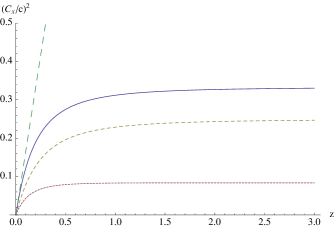
4 Final remarks

It has recently been proved the nonexistence of generic instabilities in the linearized transport equations at the Navier-Stokes regime [9]. In this paper it is shown that, in the Euler regime, there is no causality problem. The linearized transport equations become a hyperbolic system and, for further research, it can be taken as a starting point for a simplified calculation and for validation of numerical work in the non-linear case.

The non-relativistic limit has been recovered, as expected, and thermal fluctuations also satisfy a hyperbolic partial differential equation. In most textbooks, the establishment of the (parabolic) heat equation is based on an extension of Eq.(12) including heat conduction, neglecting velocity fluctuations. On the other hand, if the linearized equation of motion (15) is taken as the basis of the description of thermal fluctuations, then a causal equation is obtained for the non-dissipative fluid. Thus, for the dissipative case it is suggested that the suitable generalization of the whole linearized system (6,8,12) should be taken into account, emphasizing the role of Eq.(8) when analyzing causal properties of the system. Neglecting velocity fluctuations clearly leads to non-causality. It can be noted, also, that density fluctuations (neglecting the thermal ones) and thermal fluctuations (neglecting the density ones) present different propagation speeds, satisfying the relation $C_{n}^{2}+C_{T}^{2}=C_{s}^{2}$. Moreover, taking $\delta\theta=0$ is unrealistic, since when the fluid is at rest the mean velocity is zero, but the fluctuations do not vanish. The approximate expressions (25) and (26) may be useful in particular situations involving dissipative effects. This opens a line for future research.

The authors wish to thank A.L. Garcia-Perciante for her valuable comments for this work.

References

- [1] See for example P.F. Kolb and U. Heinz Hydrodynamic description of ultrarelativistic heavy-ion collisions in Quark Gluon Plasma 3, R.C. Hwa and X. and N. Wang Eds., World Scientific, Singapore pp 634-714 (2004) [arXiv:nucl-th/0305084] .
- [2] A. K. Chaudhuri, Phys Rev C 74, 044904 (2006)[arXiv:nucl-th/0604014].
- [3] C. Eckart, Phys. Rev. 58, 267 (1940); ibid 58, 919 (1940)
- [4] L. Landau and E.M. Lifshitz, Fluid Mechanics Addison Wesley, Reading Mass. (1958).
- [5] W. A. Hiscock and L. Lindblom; Phys. Rev. D 31, 725 (1985).
- [6] W. Israel; Ann. Phys. (N. Y.) 100, 310 (1976).
- [7] A. L. Garcia-Perciante, A. Sandoval-Villalbazo and L. S. Garcia-Colin; Gen. Rel. and Grav. (2009), online first.
- [8] C. Cercignani y G. Medeiros Kremer; The relativistic Boltzmann equation: theory and applications, Birkhäuser, Berlin (2002)
- [9] A. Sandoval-Villalbazo, A. L. Garcia-Perciante, L.S. Garcia-Colin, submitted to Physica A (2009), [Arxiv:gr-qc:0805.4237]
- [10] R. L. Liboff and R. C. Liboff; Kinetic theory: classical, quantum and relativistic descriptions, Springer, Berlin (2003).
- [11] E.W. Kolb and M.S. Turner The early universe Addison-Wesley, Reading Massachusetts(1990)