Model independent search for $Z^{\prime}$-boson signals

Abstract

An approach to the model-independent searching for the $Z^{\prime}$ gauge boson as a virtual state in scattering processes is developed. It accounts for as a basic requirement the renormalizability of underlying unspecified in other respects model. This results in a set of relations between low energy couplings of $Z^{\prime}$ to fermions that reduces in an essential way the number of parameters to be fitted in experiments. On this ground the observables which uniquely pick out the $Z^{\prime}$ boson in leptonic processes are introduced and the data of LEP experiments analyzed. The $Z^{\prime}$ couplings to leptons and quarks are estimated at 95% confidence level. These estimates may serve as a guide for experiments at the Tevatron and/or LHC. A comparison with other approaches and results is given.

1 Introduction

The precision test of the standard model (SM) at the LEP gave a possibility not only to determine all the parameters and particle masses at the level of radiative corrections but also afforded an opportunity for searching for signals of new heavy particles beyond the energy scale of it. On the base of the LEP2 experiments the low bounds on parameters of various models extending the SM have been estimated and the scale of new physics was obtained [1, 2, 3]. Although no new particles were discovered, a general believe is that the energy scale of new physics to be of order 1 TeV, that may serve as a guide for experiments at the Tevatron and LHC. In this situation, any information about new heavy particles obtained on the base of the present day data is desirable and important.

Numerous extended models include the $Z^{\prime}$ gauge boson – massive neutral vector particle associated with the extra $U(1)$ subgroup of an underlying group. Searching for this particle as a virtual state is widely discussed in the literature (see for references [4, 5]). In the content of searching for $Z^{\prime}$ at the LHC and the ILC an essential information and prospects for future investigations are given in lectures [6]. Such aspects as the mass of $Z^{\prime}$, couplings to the SM particles, $Z-Z^{\prime}$ mixing and its influence in various processes and particles parameters, distinctions between different models are discussed in details. We shall turn to these papers in what follows. As concerned a searching for $Z^{\prime}$ in the LEP experiments and the experiments at Tevatron [7], it was carried out mainly in a model-dependent way. A wide class of popular models has been investigated and low bounds on the mass $m_{Z^{\prime}}$ were estimated (see, [1, 2, 3]). As it is occurred, the low masses are varying in a wide energy interval 400-1800 GeV dependently on a specific model. These bounds are a little bit different in the LEP and Tevatron experiments. In this situation a model-independent analysis is of interest.

In the papers [8, 9, 10, 11] of the present authors a new approach for the model-independent search for $Z^{\prime}$-boson was proposed which, in contrast to other model-independent searches, gives a possibility to pick out uniquely this virtual state and determine its characteristics. The corresponding observables have also been introduced and applied to analyze the LEP2 experiment data. Our consideration is based on two constituents: 1) The relations between the effective low-energy couplings derived from the renormalization group (RG) equation for fermion scattering amplitudes. We called them the RG relations. Due to these relations, a number of unknown $Z^{\prime}$ parameters entering the amplitudes of different scattering processes considerably decreases. 2) When these relations are accounted for, some kinematics properties of the amplitude become uniquely correlated with this virtual state and the $Z^{\prime}$ signals exhibit themselves.

The RG relations allow to introduce observables correlated uniquely with the $Z^{\prime}$-boson. Comparing the mean values of the observables with the necessary specific values, one could arrive at a conclusion about the $Z^{\prime}$ existence. The confidence level (CL) of these values has been estimated and adduced in addition. Without taking into consideration the RG relations the determination of $Z^{\prime}$-boson requires a supplementary specification due to a larger number of different couplings contributing to the observables. Similar situation takes place in the “helicity model fits” of LEP Collaborations [1, 2, 3] when different virtual states contribute to each of the specific models (AA, VV, and so on). Therefore these fits had the goal to discover any signals of new physics independently of the particular states which may cause deviations from the SM. Note that the LEP Collaborations saw no indications of new contact four fermion interactions in these fits.

In Refs. [8, 10, 11] the one-parametric observables were introduced and the signals (hints in fact) of the $Z^{\prime}$ have been determined at the 1$\sigma$ CL in the $e^{+}e^{-}\to\mu^{+}\mu^{-}$ process, and at the 2$\sigma$ CL in the Bhabha process. The $Z^{\prime}$ mass was estimated to be 1–1.2 TeV. An increase in statistics could make these signals more pronounced and there is a good chance to discover this particle at the LHC.

In Ref. [12] the updated results of the one-parameter fit and the complete many-parametric fit of the LEP2 data were performed with the goal to estimate a possible signal of the $Z^{\prime}$-boson with accounting for the final data of the LEP collaborations DELPHI and OPAL [2, 3]. Usually, in a many-parametric fit the uncertainty of the result increases drastically because of extra parameters. On the contrary, in our approach due to the RG relations between the low-energy couplings there are only 2-3 independent parameters for the investigated leptonic scattering processes. As it was showed in Ref. [12], an inevitable increase of confidence areas in the many-parametric space was compensated due to accounting for all accessible experimental information. Therefore, the uncertainty of the many-parametric fit was estimated as the comparable with previous one-parametric fits in Refs. [10, 11]. In this approach the combined data fit for all lepton processes is also possible.

From the results obtained on the searching for Abelian $Z^{\prime}$ within the LEP experiment data set we conclude that it is insufficient for convincing discovery of this particle as the virtual state. In this situation it is reasonable to analyze the data by using the neural network approach which is able to make a realistic prognoses for the parameters of interest. This investigation was done within the two parametric global fit of the LEP2 data on the Bhabha scattering process. As the result of all these considerations we derive at the 2$\sigma$ CL the characteristics of the $Z^{\prime}$ (the vector $v$ and axial-vector $a$ couplings of the $Z^{\prime}$ with SM leptons and the $Z-Z^{\prime}$ mixing). The $Z^{\prime}$ mass is also estimated. Due to the universality of the $a$ we also derived the model independent estimate of the $Z^{\prime}$ axial-vector couplings to quarks, $a_{q}=a$. Note that the hints for the $Z^{\prime}$ have been determined in all the processes considered that increases the reliability of the signal. These results may serve as a good input into the future LHC and ILC experiments and used in various aspects. To underline the importance of them we mention that there are many tools at the LHC for the identification of $Z^{\prime}$. But many of them are only applicable if $Z^{\prime}$ is relatively light. The knowledge of the $Z^{\prime}$ couplings to SM fermions also have important consequences.

The paper is organized as follows. In sect. 2 we give a necessary information about the description of $Z^{\prime}$ at low energies. In sects. 3-5 we discuss the origin of the RG relations, their explicit forms for the case of the heavy $Z^{\prime}$ and consequences of the relations for scattering processes investigated. In sect. 6 the cross sections and the observables to pick out uniquely the virtual $Z^{\prime}$ in the $e^{+}e^{-}\to\mu^{+}\mu^{-},\tau^{+}\tau^{-}$ processes are given. The fits of data are described and discussed. Then in sect. 7 the same is present for the Bhabha process $e^{+}e^{-}\to e^{+}e^{-}$. The one parametric and two parametric fits are discussed. In sect. 8 the analysis of this process is carried out by using the neuron network approach. The criteria for training the network are introduced which guarantee the 2$\sigma$ CL deviations of the data from the model containing the SM with extra $Z^{\prime}$. The obtained parameters of the $Z^{\prime}$ practically coincide with that of derived in the one parameter analysis. In this way we determine the characteristics of the $Z^{\prime}$ coming from the LEP experiments. In sect. 9 we discuss the role of the present model-independent analysis for the LHC experiments. The discussion and comparison with results of other approaches are given in sect. 10. In the Appendix we describe the two-mass-scale Yukawa model and analyze in detail how the decoupling of the loop contributions due to heavy virtual states is realized when the mixing of fields is taken into consideration. This point is an essential element of the approach developed.

2 The Abelian $Z^{\prime}$ boson at low energies

Let us adduce a necessary information about the Abelian $Z^{\prime}$-boson. This particle is predicted by a number of grand unification models. Among them the $E_{6}$ and $SO(10)$ based models [13] (for instance, LR, $\chi-\psi$ and so on) are often discussed in the literature. In all the models, the Abelian $Z^{\prime}$-boson is described by a low-energy $\tilde{U}(1)$ gauge subgroup originated in some symmetry breaking pattern.

At low energies, the $Z^{\prime}$-boson can manifest itself by means of the couplings to the SM fermions and scalars as a virtual intermediate state. Moreover, the $Z$-boson couplings are also modified due to a $Z$–$Z^{\prime}$ mixing. In principle, arbitrary effective $Z^{\prime}$ interactions to the SM fields could be considered at low energies. However, the couplings of non-renormalizable types have to be suppressed by heavy mass scales because of decoupling. Therefore, significant signals beyond the SM can be inspired by the couplings of renormalizable types. Such couplings can be derived by adding new $\tilde{U}(1)$-terms to the electroweak covariant derivatives $D^{\mathrm{ew}}$ in the Lagrangian [14, 15] (review, [4, 5])

$$L_{f} = i\sum\limits_{f_{L}}\bar{f}_{L}\gamma^{\mu}\left(\partial_{\mu}-\frac{ig}{2}\sigma_{a}W^{a}_{\mu}-\frac{ig^{\prime}}{2}B_{\mu}Y_{f_{L}}-\frac{i\tilde{g}}{2}\tilde{B}_{\mu}\tilde{Y}_{f_{L}}\right)f_{L}$$

$$+ i\sum\limits_{f_{R}}\bar{f}_{R}\gamma^{\mu}\left(\partial_{\mu}-ig^{\prime}B_{\mu}Q_{f}-\frac{i\tilde{g}}{2}\tilde{B}_{\mu}\tilde{Y}_{f_{R}}\right)f_{R},$$

where summation over all the SM left-handed fermion doublets, leptons and quarks, $f_{L}={(f_{u})_{L},(f_{d})_{L}}$, and the right-handed singlets, $f_{R}=(f_{u})_{R},(f_{d})_{R}$, is understood. $Q_{f}$ denotes the charge of $f$ in positron charge units, $\tilde{Y}_{f_{L}}=\mathrm{diag}(\tilde{Y}_{f_{u}},\tilde{Y}_{f_{d}})$, and $Y_{f_{L}}=-1$ for leptons and 1/3 for quarks.

For general purposes we derive the RG relations for the $Z^{\prime}$ beyond the SM with two light Higgs doublets (THDM) [8]. $Z^{\prime}$ interactions with the scalar doublets can be parametrized in a model-independent way as follows,

$$L_{\phi}=\sum\limits_{i=1}^{2}\left|\left(\partial_{\mu}-\frac{ig}{2}\sigma_{a}W^{a}_{\mu}-\frac{ig^{\prime}}{2}B_{\mu}Y_{f_{L}}-\frac{i\tilde{g}}{2}\tilde{B}_{\mu}\tilde{Y}_{\phi_{i}}\right)\phi_{i}\right|^{2}.$$ (2)

In these formulas, $g,g^{\prime},\tilde{g}$ are the charges associated with the $SU(2)_{L},U(1)_{Y},$ and the $Z^{\prime}$ gauge groups, respectively, $\sigma_{a}$ are the Pauli matrices, $\tilde{Y}_{\phi_{i}}=\mathrm{diag}(\tilde{Y}_{\phi_{i,1}},\tilde{Y}_{\phi_{i,2}})$ is the generator corresponding to the gauge group of the $Z^{\prime}$ boson, and $Y_{\phi_{i}}$ is the $U(1)_{Y}$ hypercharge.

The Yukawa Lagrangian can be written in the form

$$L_{\mathrm{Yuk.}} = -\sqrt{2}\sum\limits_{f_{L}}\sum\limits_{i=1}^{2}\left(G_{f_{d,i}}[\bar{f}_{L}\phi_{i}(f_{d})_{R}+(\bar{f}_{d})_{R}\phi^{+}_{i}f_{L}]\right.$$ (3)

$$\left.+G_{f_{u,i}}[\bar{f}_{L}\phi_{i}^{c}(f_{u})_{R}+(\bar{f}_{u})_{R}\phi^{c+}_{i}f_{L}]\right),$$

where $\phi^{c}_{i}=i\sigma_{2}\phi^{*}_{i}$ is the charge conjugated scalar doublet.

The Lagrangian (2) leads to the $Z$–$Z^{\prime}$ mixing. The $Z$–$Z^{\prime}$ mixing angle $\theta_{0}$ is determined by the coupling $\tilde{Y}_{\phi}$ as follows

$$\theta_{0}=\frac{\tilde{g}\sin\theta_{W}\cos\theta_{W}}{\sqrt{4\pi\alpha_{\mathrm{em}}}}\frac{m^{2}_{Z}}{m^{2}_{Z^{\prime}}}\tilde{Y}_{\phi}+O\left(\frac{m^{4}_{Z}}{m^{4}_{Z^{\prime}}}\right),$$ (4)

where $\theta_{W}$ is the SM Weinberg angle, and $\alpha_{\mathrm{em}}$ is the electromagnetic fine structure constant. Although the mixing angle is a small quantity of order $m^{-2}_{Z^{\prime}}$, it contributes to the $Z$-boson exchange amplitude and cannot be neglected at the LEP energies.

In what follows we will also use the $Z^{\prime}$ couplings to the vector and axial-vector fermion currents defined as

$$v_{f}=\tilde{g}\frac{\tilde{Y}_{L,f}+\tilde{Y}_{R,f}}{2},\qquad a_{f}=\tilde{g}\frac{\tilde{Y}_{R,f}-\tilde{Y}_{L,f}}{2}.$$ (5)

The Lagrangian (2) leads to the following interactions between the fermions and the $Z$ and $Z^{\prime}$ mass eigenstates:

$${\cal L}_{Z\bar{f}f} = \frac{1}{2}Z_{\mu}\bar{f}\gamma^{\mu}\left[(v^{\mathrm{SM}}_{fZ}+\gamma^{5}a^{\mathrm{SM}}_{fZ})\cos\theta_{0}+\right.$$

$$\quad\left.+(v_{f}+\gamma^{5}a_{f})\sin\theta_{0}\right]f,$$

$${\cal L}_{Z^{\prime}\bar{f}f} = \frac{1}{2}Z^{\prime}_{\mu}\bar{f}\gamma^{\mu}\left[(v_{f}+\gamma^{5}a_{f})\cos\theta_{0}-\right.$$ (6)

$$\quad\left.-(v^{\mathrm{SM}}_{fZ}+\gamma^{5}a^{\mathrm{SM}}_{fZ})\sin\theta_{0}\right]f,$$

where $f$ is an arbitrary SM fermion state; $v^{\mathrm{SM}}_{fZ}$, $a^{\mathrm{SM}}_{fZ}$ are the SM couplings of the $Z$-boson.

Since the $Z^{\prime}$ couplings enter the cross-section together with the inverse $Z^{\prime}$ mass, it is convenient to introduce the dimensionless couplings

$$\bar{a}_{f}=\frac{m_{Z}}{\sqrt{4\pi}m_{Z^{\prime}}}a_{f},\quad\bar{v}_{f}=\frac{m_{Z}}{\sqrt{4\pi}m_{Z^{\prime}}}v_{f},$$ (7)

which can be constrained by experiments.

Low energy parameters $\tilde{Y}_{\phi_{i,1}}$, $\tilde{Y}_{\phi_{i,2}}$, $\tilde{Y}_{L,f}$, $\tilde{Y}_{R,f}$ must be fitted in experiments. In most investigations they were considered as independent ones. In a particular model, the couplings $\tilde{Y}_{\phi_{i,1}}$, $\tilde{Y}_{\phi_{i,2}},\tilde{Y}_{L,f},\tilde{Y}_{R,f}$ take some specific values. In case when the model is unknown, these parameters remain potentially arbitrary numbers. However, this is not the case if one assumes that the underlying extended model is a renormalizable one. In the papers [8, 9] it was shown that these parameters are correlated due to renormalizability. We called them the RG relations. Since this notion is a key-point of our consideration, we discuss it in detail.

3 Renormalization group relations

What is RG relation? Generally speaking, this is a correlation between low energy parameters of interactions of a heavy new particle with known light particles of the SM following from the requirement that full unknown yet theory extending SM is to be renormalizable.

Strictly speaking, RG relations are the consequence of two constituencies:

1. RG equation for a scattering amplitude;

2. Decoupling theorem.

The latter one describes the modification of both the RG operator

$${{\cal D}}=\frac{d}{d\log\mu}=\frac{\partial}{\partial\log\mu}+\sum\limits_{a}\beta_{a}\frac{\partial}{\partial\hat{\lambda}_{a}}-\sum\limits_{\hat{X}}\gamma_{X}\frac{\partial}{\partial\log\hat{X}}$$ (8)

and an amplitude at the energy threshold $\Lambda$ of new physics. Here, $\beta_{a}$- and $\gamma_{X}$-functions correspond to all the charges $\hat{\lambda}_{a}$ and fields and masses $\hat{X}$ of the underlying theory.

The RG equation for a scattering amplitude $f$ reads,

$${{\cal D}}f=\left(\frac{\partial}{\partial\log\mu}+\sum\limits_{a}\beta_{a}\frac{\partial}{\partial\hat{\lambda}_{a}}-\sum\limits_{\hat{X}}\gamma_{X}\frac{\partial}{\partial\log\hat{X}}\right)f=0,$$ (9)

where $f$ accounts for as intermediate states either the light or heavy virtual particles of the full theory. The standard usage of the RG equation is to improve the amplitude by solving this equation for the operator ${{\cal D}}$ calculated in a given order of perturbation theory. However, to search for heavy virtual particles, we will use Eq. (9) in another way.

First we note that for any renormalizable theory, the RG equation is just identity, if $f$ and ${{\cal D}}$ are calculated in a given order of loop expansion. In this case Eq. (9) expresses the well known fact that the structure of the divergent term coincides with the structure of the corresponding term in a tree-level Lagrangian.

For example, in massless QED, the tree-level plus one-loop one-particle-irreducible vertex function describing scattering of electron in an external electromagnetic field $\bar{A}$, $\Gamma=\Gamma^{(0)}+\Gamma^{(1)}$, is

If we calculate the RG operator in one-loop order

$${{\cal D}}=\frac{\partial}{\partial\log\mu}+\beta_{e}^{(1)}\frac{\partial}{\partial e}-2\gamma_{\psi}^{(1)}-\gamma_{A}^{(1)},$$ (10)

where $\beta_{e}^{(1)}$, $\gamma_{A}^{(1)},\gamma_{\psi}^{(1)}$ are the beta-function and the anomalous dimensions of electromagnetic and electron fields, respectively, and apply it to $\Gamma$, we obtain

$$-\frac{\partial}{\partial\log\mu}\Gamma^{(1)}=\left(\beta_{e}^{(1)}\frac{\partial}{\partial e}-2\gamma_{\psi}^{(1)}-\gamma_{A}^{(1)}\right)~{}\Gamma^{(0)}+O(e^{5}).$$ (11)

Then, accounting for the values of

$$\beta_{e}^{(1)}=\frac{e^{3}}{12\pi^{2}},\quad\gamma_{A}^{(1)}=\frac{e^{2}}{12\pi^{2}},\quad\gamma_{\psi}^{(1)}=\frac{e^{2}}{16\pi^{2}}$$ (12)

and the factor $e$ in $\Gamma^{(0)}$, we observe that the first and the last terms in the r.h.s. cancel. Since $\mu$-dependent term in $\Gamma^{(1)}$ is $\Gamma^{(1)}_{\mu}=\frac{e^{3}}{16\pi^{2}}\log\mu^{2}$, we see that Eq.(11) is identity in the order $O(e^{3})$.

Next important point is that in a theory with different mass scales the decoupling of heavy-loop contributions at the threshold of heavy masses, $\Lambda$, results in the following property: the running of all functions is regulated by the loops of light particles. Therefore, the $\beta$ and $\gamma$ functions at low energies are determined by the SM particles, only. This fact is the consequence of the decoupling theorem [16, 17].

The decoupling results in the redefinition of parameters at the scale $\Lambda$ and removing heavy-particle loop contributions from RG equation [18, 8]:

$$\lambda_{a} = \hat{\lambda}_{a}+a_{\hat{\lambda}_{a}}\log\frac{\hat{\Lambda}}{\mu^{2}}+b_{\hat{\lambda}_{a}}\log^{2}\frac{\Lambda^{2}}{\mu^{2}}+\cdots,$$ (13)

$$X = \hat{X}\left(1+a_{\hat{\lambda}_{a}}\log\frac{\hat{\Lambda}}{\mu^{2}}+b_{\hat{\lambda}_{a}}\log^{2}\frac{\Lambda^{2}}{\mu^{2}}+\cdots\right),$$

where $\lambda_{a}$ and $X$ denote the parameters of the SM. They are calculated assuming that no heavy particles are excited inside loops.

The matching between both sets of parameters $\lambda_{a}$, $X$ and $\hat{\lambda}_{a}$, $\hat{X}$ is chosen at the normalization point $\mu\sim\Lambda$,

$$\lambda_{a}|_{\mu=\Lambda}=\hat{\lambda}_{a}|_{\mu=\Lambda},\quad X_{a}|_{\mu=\Lambda}=\hat{X}_{a}|_{\mu=\Lambda}.$$ (14)

The differential operator ${\cal D}$ in the RG equation is in fact unique; the apparently different ${\cal D}$ in both theories are the same!

Note that if a theory with different mass scales is specified one can freely replace the parameters $\lambda_{a}$, $X$ and $\hat{\lambda}_{a}$, $\hat{X}$ by each other [18, 8].

An example of the derivation and the main features of the RG relations are shown in the Appendix for a simple model with different mass scales.

If underlying theory is not specified, the set of $\hat{\lambda}_{a}$, $\hat{X}$ is unknown. The low energy theory consists of the SM plus the effective Lagrangian generated by the interactions of light particles with virtual heavy particle states. The low energy parameters $\lambda^{\prime}_{l.}$ of these interactions are arbitrary numbers which must be constrained by experiments. By calculating the RG operator ${\cal D}$ and the scattering amplitudes of light particles in this ‘external field’ in a chosen order of loop expansion, it is possible to obtain the model-independent correlations between $\lambda^{\prime}_{l.}$. These are just the RE relations.

4 The RG relations for $Z^{\prime}$ boson couplings

Let us derive the correlations between $\tilde{Y}_{\phi_{i,1}}$, $\tilde{Y}_{\phi_{i,2}},\tilde{Y}_{L,f},\tilde{Y}_{R,f}$ appearing due to renormalizability of the underlying theory containing $Z^{\prime}$.

In our case, the RG invariance of the vertex leads to the equation

$${\cal D}\left(\bar{f}\Gamma_{fZ^{\prime}}f\frac{1}{m_{Z}^{\prime}}\right)=0,$$ (15)

where

$${{\cal D}}=\frac{d}{d\log\mu}=\frac{\partial}{\partial\log\mu}+\sum\limits_{a}\beta_{a}\frac{\partial}{\partial\lambda}_{a}-\sum\limits_{X}\gamma_{X}\frac{\partial}{\partial\log X},$$ (16)

and

$$\beta_{a}=\frac{d\lambda}{d\log\mu},~{}~{}\gamma_{X}=-\frac{d\log X}{d\log\mu}$$ (17)

are computed with taking into account the loops of light particles.

Now we derive the RG relations following from the one-loop consideration. In accordance with the previous sections, the one-loop RG equation for the vertex function reads

$$\bar{f}\frac{\partial\Gamma^{(1)}_{fZ^{\prime}}}{\partial\log\mu}f\frac{1}{m_{Z^{\prime}}}+{\cal D}^{(1)}\left(\bar{f}\Gamma^{(0)}_{fZ^{\prime}}f\frac{1}{m_{Z^{\prime}}}\right)=0,$$ (18)

where $\Gamma^{(0)}_{fZ^{\prime}}$ and $\Gamma^{(1)}_{fZ^{\prime}}$ are the tree-level and one-loop contributions to the fermion-$Z^{\prime}$ vertex. ${\cal D}^{(1)}=\sum\limits_{a}\beta^{(1)}_{a}\frac{\partial}{\partial\lambda}_{a}-\sum\limits_{X}\gamma^{(1)}_{X}\frac{\partial}{\partial\log X}$ is the one-loop level part of the RG operator.

Figure 1: The diagrams contributing to the divergent parts of the $Z^{\prime}ff$ vertex at the one-loop level.

Figure 2: The diagrams contributing to the fermion anomalous dimension at the one-loop level.

To calculate these functions, only the divergent parts of the one-loop vertices are to be calculated. The corresponding diagrams are shown in Fig. 1. The fermion anomalous dimensions $\gamma^{(1)}_{X}$ can be calculated by using the diagrams in Fig. 2. Then, Eq.(18) leads to algebraic equations for the parameters $\tilde{Y}_{\phi_{i,1}}$, $\tilde{Y}_{\phi_{i,2}},\tilde{Y}_{L,f},$ and $\tilde{Y}_{R,f}$ which have two sets of solutions [8]:

$$\tilde{Y}_{\phi_{2,1}} = \tilde{Y}_{\phi_{1,1}}=-\tilde{Y}_{\phi_{,2}}\equiv-\tilde{Y}_{\phi},$$ (19)

$$\tilde{Y}_{L,f} + \tilde{Y}_{L,f^{*}}=0,~{}\tilde{Y}_{R,f}=0,$$

and

$$\tilde{Y}_{\phi_{1,1}} = \tilde{Y}_{\phi_{2,1}}=\tilde{Y}_{\phi_{,2}}\equiv\tilde{Y}_{\phi},$$ (20)

$$\tilde{Y}_{L,f} = \tilde{Y}_{L,f^{*}},~{}~{}\tilde{Y}_{R,f}=\tilde{Y}_{L,f}+2T_{3f}~{}\tilde{Y}_{\phi}.$$

Here $f$ and $f^{*}$ are the partners of the $SU(2)_{L}$ fermion doublet ($l^{*}=\nu_{l},\nu^{*}=l,q^{*}_{u}=q_{d}$ and $q^{*}_{d}=q_{u}$), $T_{3f}$ is the third component of weak isospin.

The first of these relations describes the $Z^{\prime}$ boson analogous to the third component of the $SU(2)_{L}$ gauge field. The couplings to the right-handed singlet are absent.

The second relation corresponds to the Abelian $Z^{\prime}$. In this case the SM Lagrangian appears to be invariant with respect to the $\tilde{U}(1)$ group associated with the $Z^{\prime}$. The last relation in Eq.(20) ensures the $L_{\mathrm{Yuk.}}$ Eq.(3) is to be invariant with respect to the $\tilde{U}(1)$ transformations.

Introducing the $Z^{\prime}$ couplings to the vector and axial-vector fermion currents (5), the last line in Eq. (20) yields

$$v_{f}-a_{f}=v_{f^{*}}-a_{f^{*}},\qquad a_{f}=T_{3f}\tilde{g}\tilde{Y}_{\phi}.$$ (21)

The couplings of the Abelian $Z^{\prime}$ to the axial-vector fermion current have a universal absolute value proportional to the $Z^{\prime}$ coupling to the scalar doublet.

These relations are model independent. In particular, they hold in all the known models containing the Abelian $Z^{\prime}$. The most discussed models are derived from the ${\rm E}_{6}$ group (the so called LR, $\chi$-$\psi$ models). The tree-level $Z^{\prime}$ couplings to the SM fermions in the models are shown in Table 1.

Table 1: The $Z^{\prime}$ couplings to the SM fermions in the most discussed ${\rm E}_{6}$-based models.

$f$	$\chi$-$\psi$		LR
	$a_{f}/\tilde{g}$	$v_{f}/\tilde{g}$	$a_{f}/\tilde{g}$	$v_{f}/\tilde{g}$
$\nu$	$-3\frac{\cos{\beta}}{\sqrt{40}}-\frac{\sin{\beta}}{\sqrt{24}}$	$3\frac{\cos{\beta}}{\sqrt{40}}+\frac{\sin{\beta}}{\sqrt{24}}$	$-\frac{1}{2\alpha}$	$\frac{1}{2\alpha}$
$e$	$-\frac{\cos{\beta}}{\sqrt{10}}-\frac{\sin{\beta}}{\sqrt{6}}$	$2\frac{\cos{\beta}}{\sqrt{10}}$	$-\frac{\alpha}{2}$	$\frac{1}{\alpha}-\frac{\alpha}{2}$
$q_{u}$	$\frac{\cos{\beta}}{\sqrt{10}}-\frac{\sin{\beta}}{\sqrt{6}}$	0	$\frac{\alpha}{2}$	$-\frac{1}{3\alpha}+\frac{\alpha}{2}$
$q_{d}$	$-\frac{\cos{\beta}}{\sqrt{10}}-\frac{\sin{\beta}}{\sqrt{6}}$	$-2\frac{\cos{\beta}}{\sqrt{10}}$	$-\frac{\alpha}{2}$	$-\frac{1}{3\alpha}-\frac{\alpha}{2}$

The ${\rm E}_{6}$-symmetry breaking scheme

$${\rm E}_{6}\to{\rm SO}(10)\times{\rm U}(1)_{\psi},\quad{\rm SO}(10)\to{\rm SU}(3)_{c}\times{\rm SU}(2)_{L}\times{\rm SU}(2)_{R}\times{\rm U}(1)_{B-L}.$$

leads to the so called left-right (LR) model. Another scheme,

$${\rm E}_{6}\to{\rm SO}(10)\times{\rm U}(1)_{\psi}\to{\rm SU}(5)\times{\rm U}(1)_{\chi}\times{\rm U}(1)_{\psi},$$

predicts the Abelian $Z^{\prime}$, which is a linear combination of the neutral vector bosons $\psi$ and $\chi$,

$$Z^{\prime}=\chi\cos{\beta}+\psi\sin{\beta}$$

with the mixing angle $\beta$. If we suppose only one $Z^{\prime}$ boson at low energies, the $\psi$ boson should be much heavier than the $\chi$ field. In this case, the field $\psi$ is decoupled and $\beta\to 0$. As it is seen, both the LR and the $\chi$-$\psi$ models (with $\beta=0$ to avoid two $Z^{\prime}$ bosons with the same scale of masses) satisfy the RG relations (20) except for neutrinos. Let us explain this discrepancy. It is usually supposed in theories based on the ${\rm E}_{6}$ group that the Yukawa terms responsible for generation of the Dirac masses of neutrinos must be set to zero [13]. Therefore, the terms proportional to the Yukawa couplings vanish in the renormalization group equation, and there are no RG relations for the $Z^{\prime}$ interactions with the neutrino axial-vector currents. In this case the couplings $a_{\nu}$ given in Table 1 are not restricted by the RG relations.

5 Implication of the RG relations

LEP collaborations applied model dependent search for $Z^{\prime}$ and have obtained low bounds on the mass $m_{Z^{\prime}}\geq 400-800$ GeV dependently on a specific model [1, 2, 3].

In our analysis, we consider the SM with the additional effective $Z^{\prime}$ interactions (2), (2), (3) as a low energy theory. The parameters $a_{f},v_{f}$ and $m_{Z^{\prime}}$ must be fitted in experiments. The RG relations give a possibility:

1. reduce the number of fitted parameters;

2. determine kinematics of the processes;

3. introduce observables which uniquely pick out the $Z^{\prime}$ signals.

The RG relations (20) influences the $Z-Z^{\prime}$ mixing (4). The axial-vector coupling determines also the coupling to the scalar doublet and, consequently, the mixing angle. As a result, the number of independent couplings is significantly reduced.

In what follows, both types of the RG relations (19) and (20) will be used in order to search for signals of the $Z^{\prime}$ gauge boson.

6 $Z^{\prime}$ search in $e^{+}e^{-}\to\mu^{+}\mu^{-},\tau^{+}\tau^{-}$ processes

6.1 The differential cross section

Let us consider the processes $e^{+}e^{-}\to l^{+}l^{-}$ ($l=\mu,\tau$) with the non-polarized initial- and final-state fermions. In order to introduce the observable which selects the signal of the Abelian $Z^{\prime}$ boson we need to compute the differential cross-sections of the processes up to the one-loop level.

The lower-order diagrams describe the neutral vector boson exchange in the $s$-channel ($e^{+}e^{-}\to V^{\ast}\to l^{+}l^{-}$, $V=A,Z,Z^{\prime}$). As for the one-loop corrections, two classes of diagrams are taken into account. The first one includes the pure SM graphs (the mass operators, the vertex corrections, and the boxes). The second set of the one-loop diagrams improves the Born-level $Z^{\prime}$-exchange amplitude by “dressing” the $Z^{\prime}$ propagator and and the $Z^{\prime}$–fermion vertices. We assume that $Z^{\prime}$ states are not excited inside loops. Such an approximation means that the $Z^{\prime}$-boson is completely decoupled. Then, the differential cross-section consists of the squared tree-level amplitude and the term from the interference of the tree-level and the one-loop amplitudes. To obtain an infrared-finite result, we also take into account the processes with the soft-photon emission in the initial and final states.

In the lower order in $m^{-2}_{Z^{\prime}}$ the $Z^{\prime}$ contributions to the differential cross-section of the process $e^{+}e^{-}\to l^{+}l^{-}$ are expressed in terms of four-fermion contact couplings, only. If one takes into consideration the higher-order corrections in $m^{-2}_{Z^{\prime}}$, it becomes possible to estimate separately the $Z^{\prime}$-induced contact couplings and the $Z^{\prime}$ mass [19]. In the present analysis we keep the terms of order $O(m^{-4}_{Z^{\prime}})$ to fit both of these parameters.

Expanding the differential cross-section in the inverse $Z^{\prime}$ mass and neglecting the terms of order $O(m^{-6}_{Z^{\prime}})$, we have

$$\frac{d\sigma_{l}(s)}{dz} = \frac{d\sigma_{l}^{\rm SM}(s)}{dz}+\sum_{i=1}^{7}\sum_{j=1}^{i}\left[A_{ij}^{l}(s,z)+B_{ij}^{l}(s,z)\zeta\right]x_{i}x_{j}$$ (22)

$$+\sum_{i=1}^{7}\sum_{j=1}^{i}\sum_{k=1}^{j}\sum_{n=1}^{k}C_{ijkn}^{l}(s,z)x_{i}x_{j}x_{k}x_{n},$$

where the dimensionless quantities

$$\zeta=\frac{m^{2}_{Z}}{m^{2}_{Z^{\prime}}},\quad(x_{1},x_{2},x_{3},x_{4},x_{5},x_{6},x_{7})=(\bar{a},\bar{v}_{e},\bar{v}_{\mu},\bar{v}_{\tau},\bar{v}_{d},\bar{v}_{s},\bar{v}_{b})$$ (23)

are introduced. Since the axial-vector couplings of the Abelian $Z^{\prime}$ boson are universal, we use the shorthand notation $\bar{a}=\bar{a}_{e}$. In what follows the index $l=\mu,\tau$ denotes the final-state lepton.

The coefficients $A$, $B$, $C$ are determined by the SM couplings and masses. Each factor may include the tree-level contribution, the one-loop correction and the term describing the soft-photon emission. The factors $A$ describe the leading-order contribution, whereas others correspond to the higher order corrections in $m^{-2}_{Z^{\prime}}$.

6.2 The observable

To take into consideration the correlations (4) we introduce the observable $\sigma_{l}(z)$ defined as the difference of cross sections integrated in some ranges of the scattering angle $\theta$ [9, 10]:

$$\sigma_{l}(z) \equiv \int\nolimits_{z}^{1}\frac{d\sigma_{l}}{d\cos\theta}d\cos\theta-\int\nolimits_{-1}^{z}\frac{d\sigma_{l}}{d\cos\theta}d\cos\theta,$$ (24)

where $z$ stands for the cosine of the boundary angle. The idea of introducing the $z$-dependent observable (24) is to choose the value of the kinematic parameter $z$ in such a way that to pick up the characteristic features of the Abelian $Z^{\prime}$ signals.

The deviation of the observable from its SM value can be derived by the angular integration of the differential cross-section and has the form:

$$\Delta\sigma_{l}(z) = \sigma_{l}(z)-\sigma^{\rm SM}_{l}(z)=\sum_{i=1}^{7}\sum_{j=1}^{i}\left[\tilde{A}_{ij}^{l}(s,z)+\tilde{B}_{ij}^{l}(s,z)\zeta\right]x_{i}x_{j}$$ (25)

$$+\sum_{i=1}^{7}\sum_{j=1}^{i}\sum_{k=1}^{j}\sum_{n=1}^{k}\tilde{C}_{ijkn}^{l}(s,z)x_{i}x_{j}x_{k}x_{n}.$$

Then let us introduce the quantity $\Delta\sigma\left(z\right)\equiv\sigma\left(z\right)-{\sigma}_{SM}\left(z\right)$, which owing to the relations (20) can be written in the form

$$\Delta\sigma_{f}(z) = \frac{\alpha N_{f}}{8}\frac{g^{2}_{Z^{\prime}}}{m^{2}_{Z^{\prime}}}\left[F^{f}_{0}(z,s)\tilde{Y}^{2}_{\phi}+2F^{f}_{1}(z,s)T_{3f}\tilde{Y}_{L,f}\tilde{Y}_{L,e}\right.$$ (26)

$$+\left.2F^{f}_{2}(z,s)T_{3f}\tilde{Y}_{L,f}\tilde{Y}_{\phi}+F^{f}_{3}(z,s)\tilde{Y}_{L,e}\tilde{Y}_{\phi}\right].$$

The factor functions $F^{f}_{i}(z,s)$ depend on the fermion type through the $|Q_{f}|$, only. In Fig. 3 they are shown as the functions of $z$ for $\sqrt{s}=500$ GeV. The leading contributions to $F^{f}_{i}(z,s)$,

$$F^{f}_{0}(z,s) = -\frac{4}{3}\left|Q_{f}\right|\left(1-z-z^{2}-\frac{z^{3}}{3}\right)+O\left(\frac{m^{2}_{Z}}{s}\right),$$

$$F^{f}_{1}(z,s) = \frac{4}{3}\left[1-z^{2}-\left|Q_{f}\right|\left(3z+z^{3}\right)\right]+O\left(\frac{m^{2}_{Z}}{s}\right),$$

$$F^{f}_{2}(z,s) = -\frac{2}{3}\left(1-z^{2}\right)+\frac{2}{9}\left(3z+z^{3}\right)\left(4\left|Q_{f}\right|-1\right)+O\left(\frac{m^{2}_{Z}}{s}\right),$$

$$F^{f}_{3}(z,s) = \frac{2}{3}\left|Q_{f}\right|\left(1-3z-z^{2}-z^{3}\right)+O\left(\frac{m^{2}_{Z}}{s}\right),$$ (27)

are given by the $Z^{\prime}$ exchange diagram $e^{-}e^{+}\to Z^{\prime}\to\bar{f}f$, since the $Z$-$Z^{\prime}$ mixing contribution to the $Z$ exchange diagram is suppressed by the factor $m^{2}_{Z}/s$.

Figure 3: The leptonic functions $F^{l}_{0}$ (the solid curve), $F^{l}_{1}$ (the long-dashed curve), $F^{l}_{2}$ (the dashed curve), and $F^{l}_{3}$ (the dotted curve) at $\sqrt{s}=500$ GeV.

From Eqs. (6.2) one can see that the leading contributions to the leptonic factors $F^{l}_{1}$, $F^{l}_{2}$, $F^{l}_{3}$ are found to be proportional to the same polynomial in $z$. This is the characteristic feature of the leptonic functions $F^{l}_{i}$ originating due to the kinematic properties of fermionic currents and the specific values of the SM leptonic charges. Therefore, it is possible to choose the value of $z=z^{\ast}$ which switches off three leptonic factors $F^{l}_{1}$, $F^{l}_{2}$, $F^{l}_{3}$ simultaneously. Moreover, the quark function $F^{q}_{3}$ in the lower order is proportional to the leptonic one and therefore is switched off, too. As is seen from Fig. 3, the appropriate value of $z^{\ast}$ is about $\sim 0.3$. By choosing this value of $z^{\ast}$ one can simplify Eq. (26). It is also follows from Eq. (26) that neglecting the factors $F^{l}_{1}$, $F^{l}_{2}$, $F^{l}_{3}$ one obtains the sign definite quantity $\Delta\sigma_{l}(z^{\ast})\sim\tilde{Y}^{2}_{\phi}\sim\bar{a}^{2}$.

There is an interval of values of the boundary angle, at which the factors $\tilde{A}^{l}_{11}$, $\tilde{B}^{l}_{11}$, and $\tilde{C}^{l}_{1111}$ at the sign-definite parameters $\bar{a}^{2}$, $\bar{a}^{2}\zeta$, and $\bar{a}^{4}$ contribute more than 95% of the observable value. It gives a possibility to construct the sign-definite observable $\Delta\sigma_{l}(z^{*})<0$ by specifying the proper value of $z^{*}$.

In general, one could choose the boundary angle $z^{*}$ in different schemes. If just a few number of tree-level four-fermion contact couplings are considered, one can specify $z^{*}$ in order to cancel the factor at the vector-vector coupling. However, if one-loop corrections are taken into account there are a large number of additional contact couplings. So, we have to define some quantitative criterion $F(z)$ to estimate the contributions from sign-definite factors at a given value of the boundary angle $z$. Maximizing the criterion, one could derive the value $z^{*}$, which corresponds to the sign-definite observable $\Delta\sigma_{l}(z^{*})$. Since the observable is linear in the coefficients $A$, $B$, and $C$, we introduce the following criterion,

$$F=\frac{|\tilde{A}_{11}|+\omega_{B}|\tilde{B}_{11}|+\omega_{C}|\tilde{C}_{1111}|}{\sum\limits_{{\rm all}~{}\tilde{A}}\left|\tilde{A}_{ij}\right|+\omega_{B}\sum\limits_{{\rm all}~{}\tilde{B}}\left|\tilde{B}_{ij}\right|+\omega_{C}\sum\limits_{{\rm all}~{}\tilde{C}}\left|\tilde{C}_{ijkn}\right|},$$ (28)

where the positive ‘weights’ $\omega_{B}\sim\zeta$ and $\omega_{C}\sim\epsilon$ take into account the order of each term in the inverse $Z^{\prime}$ mass.

The numeric values of the ‘weights’ $\omega_{B}$ and $\omega_{C}$ can be taken from the present day bounds on the contact couplings [1]. As the computation shows, the value of $z^{*}$ with the accuracy $10^{-3}$ depends on the order of the ‘weight’ magnitudes, only. So, in what follows we take $\omega_{B}\sim 4\times 10^{-3}$ and $\omega_{C}\sim 4\times 10^{-5}$.

The function $z^{\ast}(s)$ is the decreasing function of the center-of-mass energy. It is tabulated for the LEP2 energies in Table 2. The corresponding values of the maximized function $F$ are within the interval $0.95<F<0.96$.

Table 2: The boundary angle $z^{*}$ and the coefficients in the observable $\Delta\sigma_{l}(z^{*})$ for the scattering into $\mu$ and $\tau$ pairs at the one-loop level.

	$\mu^{+}\mu^{-}$				$\tau^{+}\tau^{-}$
$\sqrt{s}$, GeV	$z^{*}$	$\tilde{A}_{11}$	$\tilde{B}_{11}$	$\tilde{C}_{1111}$	$z^{*}$	$\tilde{A}_{11}$	$\tilde{B}_{11}$	$\tilde{C}_{1111}$
130	0.450	-729	-1792	-19636	0.460	-687	-1664	-25782
136	0.439	-709	-1859	-16880	0.442	-688	-1779	-20784
161	0.400	-643	-2183	-6890	0.400	-625	-2097	-10993
172	0.390	-619	-4099	-4099	0.391	-601	-2263	-8382
183	0.383	-599	-2545	-1334	0.385	-571	-2402	-7580
189	0.380	-586	-2635	-495	0.380	-568	-2533	-5135
192	0.380	-579	-2681	-63	0.380	-562	-2578	-4769
196	0.380	-571	-2745	-528	0.379	-554	-2640	-4272
200	0.378	-564	-2811	-1137	0.378	-547	-2704	-3761
202	0.376	-560	-2845	-1448	0.377	-543	-2736	-3501
205	0.374	-555	-2897	-1923	0.374	-548	-2834	-1292
207	0.372	-552	-2932	-2245	0.372	-544	-2868	-1010

Since $\tilde{A}^{l}_{11}(s,z^{*})<0$, $\tilde{B}^{l}_{11}(s,z^{*})<0$ and $\tilde{C}^{l}_{1111}(s,z^{*})<0$, the observable

$$\Delta\sigma_{l}(z^{*})=\left[\tilde{A}^{l}_{11}(s,z^{*})+\zeta\tilde{B}^{l}_{11}(s,z^{*})\right]\bar{a}^{2}+\tilde{C}^{l}_{1111}(s,z^{*})\bar{a}^{4}$$ (29)

is negative with the accuracy 4–5%. Since this property follows from the RG relations (4) for the Abelian $Z^{\prime}$ boson, the observable $\Delta\sigma_{l}(z^{*})$ selects the model-independent signal of this particle in the processes $e^{+}e^{-}\to l^{+}l^{-}$. It allows to use the data on scattering into $\mu\mu$ and $\tau\tau$ pairs in order to estimate the Abelian $Z^{\prime}$ coupling to the axial-vector lepton currents.

Although the observable can be computed from the differential cross-sections directly, it is also possible to recalculate it from the total cross-sections and the forward-backward asymmetries. The recalculation procedure has the proper theoretical accuracy. Nevertheless, it allows to reduce the experimental errors on the observable, since the published data on the total cross-sections and the forward-backward asymmetries are more precise than the data on the differential cross-sections.

The recalculation is based on the fact that the differential cross-section can be approximated with a good accuracy by the two-parametric polynomial in the cosine of the scattering angle $z$:

$$\frac{d\sigma_{l}(s)}{dz}=\frac{d\sigma_{l}^{\rm SM}(s)}{dz}+(1+z^{2})\beta_{l}+z\eta_{l}+\delta_{l}(z),$$ (30)

where $\delta_{l}(z)$ measures the difference between the exact and the approximated cross-sections. The approximated cross-section reproduces the exact one in the limit of the massless initial- and final-state leptons and if one neglects the contributions of the box diagrams.

Performing the angular integration, it is easy to obtain the expression for the observable:

$$\Delta\sigma_{l}(z^{*})=\sigma_{l}(z^{*})-\sigma_{l}^{\rm SM}(z^{*})=(1-z^{*2})\eta_{l}-\frac{2\beta_{l}}{9}z^{*}(3+z^{*2})+\tilde{\delta}_{l}(z^{*}),$$ (31)

and for the total and the forward-backward cross-sections:

$$\Delta\sigma^{\rm T}_{l} = \sigma^{\rm T}_{l}-\sigma_{l}^{\rm T,SM}=\frac{8\beta_{l}}{9}+\tilde{\delta}_{l}(-1),$$

$$\Delta\sigma^{\rm FB}_{l} = \sigma^{\rm FB}_{l}-\sigma_{l}^{\rm FB,SM}=\eta_{l}+\tilde{\delta}_{l}(0).$$ (32)

Then, the factors $\beta_{l}$ and $\eta_{l}$ can be eliminated from the observable:

$$\Delta\sigma_{l}(z^{*}) = (1-z^{*2})\Delta\sigma^{\rm FB}_{l}-\frac{3}{12}z^{*}(3+z^{*2})\Delta\sigma^{\rm T}_{l}+\xi_{l}.$$ (33)

The quantity $\xi_{l}$,

$$\xi_{l} = \tilde{\delta}_{l}(z^{*})-(1-z^{*2})\tilde{\delta}_{l}(0)+\frac{3}{12}z^{*}(3+z^{*2})\tilde{\delta}_{l}(-1),$$ (34)

measures the theoretical accuracy of the approximation.

The forward-backward cross-section is related to the total one and the forward-backward asymmetry by means of the following expression

$$\Delta\sigma^{\rm FB}_{l} = \Delta\sigma^{\rm T}_{l}\,\,A^{\rm FB}_{l}+\sigma_{l}^{\rm T,SM}\,\,\Delta A^{\rm FB}_{l}.$$ (35)

As the computation shows, $\tilde{\delta}_{l}(z^{*})\simeq 0.01\Delta\sigma_{l}(z^{*})$, $\tilde{\delta}_{l}(0)\simeq 0.007\Delta\sigma^{\rm FB}_{l}$, and $\tilde{\delta}_{l}(-1)\simeq-0.07\Delta\sigma^{\rm T}_{l}$ at the LEP2 energies. Taking into account the experimental values of the total cross-sections and the forward-backward asymmetries at the LEP2 energies ($\Delta\sigma^{\rm T}_{l}\simeq 0.1$pb, $\sigma_{l}^{\rm T,SM}\simeq 2.7$pb, $\Delta A_{l}^{\rm FB}\simeq 0.04$, $A_{l}^{\rm FB}\simeq 0.5$), one can estimate the theoretical error as $\xi_{l}\simeq 0.003{\rm pb}$. At the same time, the corresponding statistical uncertainties on the observable are larger than 0.06pb. Thus, the proposed approximation is quite good and can be successfully used to obtain more accurate experimental values of the observable.

6.3 Data fit

To search for the model-independent signals of the Abelian $Z^{\prime}$-boson we will analyze the introduced observable $\Delta\sigma_{l}(z^{\ast})$ on the base of the LEP2 data set. In the lower order in $m^{-2}_{Z^{\prime}}$ the observable (29) depends on one flavor-independent parameter $\bar{a}^{2}$,

$$\Delta\sigma^{\rm th}_{l}(z^{*})=\tilde{A}^{l}_{11}(s,z^{*})\bar{a}^{2}+\tilde{C}^{l}_{1111}(s,z^{*})\bar{a}^{4},$$ (36)

which can be fitted from the experimental values of $\Delta\sigma_{\mu}(z^{\ast})$ and $\Delta\sigma_{\tau}(z^{\ast})$. As we noted above, the sign of the fitted parameter ($\bar{a}^{2}>0$) is a characteristic feature of the Abelian $Z^{\prime}$ signal.

In what follows we will apply the usual fit method based on the likelihood function. The central value of $\bar{a}^{2}$ is obtained by the minimization of the $\chi^{2}$-function:

$$\chi^{2}(\bar{a}^{2})=\sum_{n}\frac{\left[\Delta\sigma^{\rm ex}_{\mu,n}(z^{*})-\Delta\sigma^{\rm th}_{\mu}(z^{*})\right]^{2}}{\delta\sigma^{\rm ex}_{\mu,n}(z^{*})^{2}},$$ (37)

where the sum runs over the experimental points entering a data set chosen. The $1\sigma$ CL interval $(b_{1},b_{2})$ for the fitted parameter is derived by means of the likelihood function ${\cal L}(\bar{a}^{2})\propto\exp[-\chi^{2}(\bar{a}^{2})/2]$. It is determined by the equations:

$$\int\nolimits_{b_{1}}^{b_{2}}{\cal L}(\epsilon^{\prime})d\epsilon^{\prime}=0.68,\quad{\cal L}(b_{1})={\cal L}(b_{2}).$$ (38)

To compare our results with those of Refs. [1] we introduce the contact interaction scale

$$\Lambda^{2}=4m^{2}_{Z}\bar{a}^{-2}.$$ (39)

This normalization of contact couplings is admitted in Refs. [1]. We use again the likelihood method to determine a one-sided lower limit on the scale $\Lambda$ at the 95% CL. It is derived by the integration of the likelihood function over the physically allowed region $\bar{a}^{2}>0$. The strict definition is

$$\Lambda=2m_{Z}(\epsilon^{*})^{-1/2},\quad\int_{0}^{\epsilon^{*}}{\cal L}(\epsilon^{\prime})d\epsilon^{\prime}=0.95\int_{0}^{\infty}{\cal L}(\epsilon^{\prime})d\epsilon^{\prime}.$$ (40)

We also introduce the probability of the Abelian $Z^{\prime}$ signal as the integral of the likelihood function over the positive values of $\bar{a}^{2}$:

$$P=\int\nolimits_{0}^{\infty}L(\epsilon^{\prime})d\epsilon^{\prime}.$$ (41)

Actually, the fitted value of the contact coupling $\bar{a}^{2}$ originates mainly from the leading-order term in the inverse $Z^{\prime}$ mass in Eq. (29). The analysis of the higher-order terms allows to estimate the constraints on the $Z^{\prime}$ mass alone. Substituting $\bar{a}^{2}$ in the observable (29) by its fitted central value, one obtains the expression

$$\Delta\sigma_{l}(z^{*})=\left[\tilde{A}^{l}_{11}(s,z^{*})+\zeta\tilde{B}^{l}_{11}(s,z^{*})\right]\bar{a}_{\mathrm{fitted}}^{2}+\tilde{C}^{l}_{1111}(s,z^{*})\bar{a}_{\mathrm{fitted}}^{4},$$ (42)

which depends on the parameter $\zeta=m^{2}_{Z}/m^{2}_{Z^{\prime}}$. Then, the central value of this parameter and the corresponding 1$\sigma$ CL interval are derived in the same way as those for $\bar{a}^{2}$.

To fit the parameters $\bar{a}^{2}$ and $\zeta$ we start with the LEP2 data on the total cross-sections and the forward-backward asymmetries [1]. The corresponding values of the observable $\Delta\sigma_{l}(z^{\ast})$ with their uncertainties $\delta\sigma_{l}(z^{\ast})$ are calculated from the data by means of the following relations:

$$\Delta\sigma_{l}(z^{\ast}) = \left[A_{l}^{\rm FB}\left(1-z^{\ast 2}\right)-\frac{z^{\ast}}{4}\left(3+z^{\ast 2}\right)\right]\Delta\sigma_{l}^{\rm T}$$

$$+\left(1-z^{\ast 2}\right)\sigma_{l}^{\rm T,SM}\Delta A_{l}^{\rm FB},$$

$$\delta\sigma_{l}(z^{\ast})^{2} = {\left[A_{l}^{\rm FB}\left(1-z^{\ast 2}\right)-\frac{z^{\ast}}{4}\left(3+z^{\ast 2}\right)\right]}^{2}(\delta\sigma_{l}^{\rm T})^{2}$$ (43)

$$+{\left[\left(1-z^{\ast 2}\right)\sigma_{l}^{\rm T,SM}\right]}^{2}(\delta A_{l}^{\rm FB})^{2}.$$

We perform the fits assuming several data sets, including the $\mu\mu$, $\tau\tau$, and the complete $\mu\mu$ and $\tau\tau$ data, respectively. The results are presented in Table 3.

Table 3: The contact coupling $\bar{a}^{2}$ with the 68% CL uncertainty, the 95% CL lower limit on the scale $\Lambda$, the probability of the $Z^{\prime}$ signal, $P$, and the value of $\zeta=m^{2}_{Z}/m^{2}_{Z^{\prime}}$ as a result of the fit of the observable recalculated from the total cross-sections and the forward-backward asymmetries.

Data set	$\bar{a}^{2}$	$\Lambda$, TeV	$P$	$\zeta$
$\mu\mu$	$0.0000366^{+0.0000489}_{-0.0000486}$	16.4	0.77	$0.009\pm 0.278$
$\tau\tau$	$-0.0000266^{+0.0000643}_{-0.0000639}$	17.4	0.34	$-0.001\pm 0.501$
$\mu\mu$ and $\tau\tau$	$0.0000133^{+0.0000389}_{-0.0000387}$	19.7	0.63	$0.017\pm 0.609$

As is seen, the more precise $\mu\mu$ data demonstrate the signal of about 1$\sigma$ level. It corresponds to the Abelian $Z^{\prime}$-boson with the mass of order 1.2–1.5 TeV if one assumes the value of $\tilde{\alpha}=\tilde{g}^{2}/4\pi$ to be in the interval 0.01–0.02. No signal is found by the analysis of the $\tau\tau$ cross-sections. The combined fit of the $\mu\mu$ and $\tau\tau$ data leads to the signal below the 1$\sigma$ CL.

Being governed by the next-to-leading contributions in $m^{-2}_{Z^{\prime}}$, the fitted values of $\zeta$ are characterized by significant errors. The $\mu\mu$ data set gives the central value which corresponds to $m_{Z^{\prime}}\simeq 1.1$ TeV.

We also perform a separate fit of the parameters based on the direct calculation of the observable from the differential cross-sections. The experimental uncertainties of the data on the differential cross-sections are of one order larger than the corresponding errors of the total cross-sections and the forward-backward asymmetries. These data also provide the larger values of the contact coupling $\bar{a}^{2}$. As for the more precise $\mu\mu$ data, three of the LEP2 Collaborations demonstrate positive values of $\bar{a}^{2}$. The combined $\bar{a}^{2}$ is also positive and remains practically unchanged by the incorporation of the $\tau\tau$ data.

As it was mentioned in the previous section, the indirect computation of the observable from the total cross-sections and the forward-backward asymmetries inspires some insufficient theoretical uncertainty about 2% of the statistical one. It also increases the statistical error because of the recalculation procedure. Nevertheless, the uncertainty of the fitted parameter $\bar{a}^{2}$ within the recalculation scheme is of one order less than that for the direct computation from the differential cross-sections. This difference is explained by the different accuracy of the available experimental data on the differential and the total cross-sections.

7 Search for $Z^{\prime}$ in $e^{+}e^{-}\to e^{+}e^{-}$ process

7.1 The differential cross-section

In our analysis, as the SM values of the cross-sections we use the quantities calculated by the LEP2 collaborations [2, 3, 20, 21]. They account for either the one-loop radiative corrections or initial and final state radiation effects (together with the event selection rules, which are specific for each experiment). As it is reported by the DELPHI Collaboration, there is a theoretical error of the SM values of about 2%. In our analysis this error is added to the statistical and systematic ones for all the Collaborations. As it was checked, the fit results are practically insensitive to accounting for this error.

The deviation from the SM is computed in the improved Born approximation. This approximation is sufficient for our analysis leading to the systematic error of the fit results less than 5-10 per cents.

The deviation from the SM of the differential cross-section for the process $e^{+}e^{-}\to\ell^{+}\ell^{-}$ can be expressed through various quadratic combinations of couplings $a=a_{e}$, $v_{e}$, $v_{\mu}$, $v_{\tau}$. For the Bhabha process it reads

$$\frac{d\sigma}{dz}-\frac{d\sigma^{\mathrm{SM}}}{dz}=f^{ee}_{1}(z)\frac{a^{2}}{m_{Z^{\prime}}^{2}}+f^{ee}_{2}(z)\frac{v_{e}^{2}}{m_{Z^{\prime}}^{2}}+f^{ee}_{3}(z)\frac{av_{e}}{m_{Z^{\prime}}^{2}},$$ (44)

where the factors are known functions of the center-of-mass energy and the cosine of the electron scattering angle $z$ plotted in Fig. 4.

Figure 4: The factors at the $Z^{\prime}$ couplings in the differential cross-section of the Bhabha process.

The deviation of the cross-section for $e^{+}e^{-}\to\mu^{+}\mu^{-}$ ($\tau^{+}\tau^{-}$) processes has a similar form

$$\frac{d\sigma}{dz}-\frac{d\sigma^{\mathrm{SM}}}{dz} = f^{\mu\mu}_{1}(z)\frac{a^{2}}{m_{Z^{\prime}}^{2}}+f^{\mu\mu}_{2}(z)\frac{v_{e}v_{\mu}}{m_{Z^{\prime}}^{2}}+$$ (45)

$$+f^{\mu\mu}_{3}(z)\frac{av_{e}}{m_{Z^{\prime}}^{2}}+f^{\mu\mu}_{4}(z)\frac{av_{\mu}}{m_{Z^{\prime}}^{2}}.$$

Eqs. (44)–(45) are our definition of the $Z^{\prime}$ signal.

Note again that the cross-sections in Eqs. (44)–(45) account for the relations (62) through the functions $f_{1}(z)$, $f_{3}(z)$, $f_{4}(z)$, since the coupling $\tilde{Y}_{\phi}$ (the mixing angle $\theta_{0}$) is substituted by the axial coupling constant $a$. Usually, when a four-fermion effective Lagrangian is applied to describe physics beyond the SM [22], this dependence on the scalar field coupling is neglected at all. However, in our case, when we are interested in searching for signals of the $Z^{\prime}$-boson on the base of the effective low-energy Lagrangian (2)–(3), these contributions to the cross-section are essential.

7.2 One-parameter fit

The factor $f^{ee}_{2}(z)$ is positive monotonic function of $z$ (see Fig. 4 for the center-of-mass energies $\sqrt{s}=200$ GeV. The same behavior is observed for higher energies). Such a property allows one to choose $f^{ee}_{2}(z)$ as a normalization factor for the differential cross section. Then the normalized deviation of the differential cross-section reads [11]

$$\frac{d\tilde{\sigma}}{dz} = \frac{m_{Z}^{2}}{{4\pi}f^{ee}_{2}(z)}\Delta\,\frac{d\sigma}{dz}=$$ (46)

$$\bar{v}^{2}+F_{a}(\sqrt{s},z)\bar{a}^{2}+F_{av}(\sqrt{s},z)\bar{a}\bar{v}+\ldots,$$

and the normalized factors are shown in Fig 5.

Figure 5: Factors $F_{a}(\sqrt{s},z)$ (solid) and $F_{av}(\sqrt{s},z)$ (dashed) in the normalized deviation of the differential cross-section $d\tilde{\sigma}/dz$ for $\sqrt{s}=200$ and 500 GeV.

Now these factors are finite at $z\to 1$. Each of them in a special way influences the differential cross-section.

1. The factor at $\bar{v}^{2}$ is just the unity. Hence, the four-fermion contact coupling between vector currents, $\bar{v}^{2}$, determines the level of the deviation from the SM value.

2. The factor at $\bar{a}^{2}$ depends on the scattering angle in a non-trivial way. It allows to recognize the Abelian $Z^{\prime}$ boson, if the experimental accuracy is sufficient.

3. The factor at $\bar{a}\bar{v}$ results in small corrections.

Thus, effectively, the obtained normalized differential cross-section is a two-parametric function. In the next sections we introduce the observables to fit separately each of these parameters.

7.3 Observables to pick out $\bar{v}^{2}$

To recognize the signal of the Abelian $Z^{\prime}$ boson by analyzing the Bhabha process the differential cross-section deviation from the SM predictions should be measured with a good accuracy. At present, no such deviations have been detected at more than the 1$\sigma$ CL. In this situation it is resonable to introduce integrated observables allowing to pick out $Z^{\prime}$ signals by using the most effective treating of available data. The observables should be sensitive to the separate $Z^{\prime}$ couplings. This admits of searching for the $Z^{\prime}$ signals in different processes as well as to perform global fits.

The normalized deviation of the differential cross-section (46) is (effectively) the function of two parameters, $\bar{a}^{2}$ and $\bar{v}^{2}$. We are going to introduce the integrated observables which determine separately the four-fermion couplings $\bar{a}^{2}$ and $\bar{v}^{2}$ [11].

Let us first proceed with the observable for $\bar{v}^{2}$. After normalization the factor at the vector-vector four-fermion coupling becomes the unity. Whereas the factor at $\bar{a}^{2}$ is a sign-varying function of the cosine of the scattering angle. As it follows from Fig. 5, for the center-of-mass energy 200 GeV it is small over the backward scattering angles. So, to measure the value of $\bar{v}^{2}$ the normalized deviation of the differential cross-section has to be integrated over the backward angles. For the center-of-mass energy 500 GeV the factor at $\bar{a}^{2}$ is already a non-vanishing quantity for the backward scattering angles. The curves corresponding to intermediate energies are distributed in between two these curves. Since they are sign-varying ones at each energy point some interval of $z$ can be chosen to make the integral to be zero. Thus, to measure the $Z^{\prime}$ coupling to the electron vector current $\bar{v}^{2}$ we introduce the integrated cross-section (46)

$$\sigma_{V}=\int_{z_{0}}^{z_{0}+\Delta z}(d\tilde{\sigma}/dz)dz,$$ (47)

where at each energy the most effective interval $[z_{0},z_{0}+\Delta z]$ is determined by the following requirements:

1. The relative contribution of the coupling $\bar{v}^{2}$ is maximal. Equivalently, the contribution of the factor at $\bar{a}^{2}$ is suppressed.

2. The length $\Delta z$ of the interval is maximal. This condition ensures that the largest number of bins is taken into consideration.

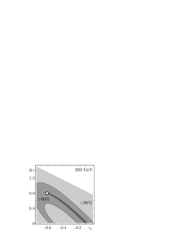
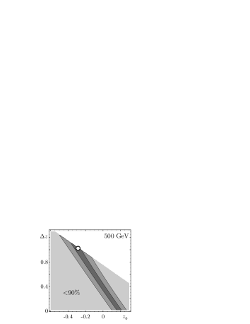
Figure 6: Relative contribution of the factor at $\bar{v}^{2}$ to the observable $\sigma_{V}$ as the function of the left boundary of the angle interval, $z_{0}$, and the interval length, $\Delta z$, at the center-of-mass energy 200 and 500 GeV. The shaded areas correspond to the contributions $>95\%$ (dark), from 90% to 95% (midtone), and $<90\%$ (light).

The relative contribution of the factor at $\bar{v}^{2}$ is defined as

$$\kappa_{V}=\frac{\Delta z}{\Delta z+\left|\int_{z_{0}}^{z_{0}+\Delta z}F_{a}\,dz\right|+\left|\int_{z_{0}}^{z_{0}+\Delta z}F_{av}\,dz\right|}$$ (48)

and shown in Fig. 6 as the function of the left boundary of the angle interval, $z_{0}$, and the interval length, $\Delta z$. In each plot the dark area corresponds to the observables which values are determined by the vector-vector coupling $\bar{v}^{2}$ with the accuracy $>95\%$. The area reflects the correlation of the width of the integration interval $\Delta z$ with the choice of the initial $z_{0}$ following from the mentioned requirements. Within this area we choose the observable which includes the largest number of bins (largest $\Delta z$). The corresponding values of $z_{0}$ and $\Delta z$ are marked by the white dot on the plots in Fig. 6. As the carried out analysis showed, the point $z_{0}$ is shifted to the right with increase in energy whereas $\Delta z$ remains approximately the same.

From the plots it follows that the most efficient intervals are

$$-0.6<z<0.2,\quad\sqrt{s}=200\mbox{ GeV},$$

$$-0.3<z<0.7,\quad\sqrt{s}=500\mbox{ GeV}.$$ (49)

Therefore the observable (47) allows to measure the $Z^{\prime}$ coupling to the electron vector current $\bar{v}^{2}$ with the efficiency $>95\%$.

Fitting the LEP2 final data with the one-parameter observable, we find the values of the $Z^{\prime}$ coupling to the electron vector current together with their 1$\sigma$ uncertainties:

$$\mathrm{ALEPH}: \bar{v}_{e}^{2}= -0.11\pm 6.53\times 10^{-4}$$

$$\mathrm{DELPHI}: \bar{v}_{e}^{2}= 1.60\pm 1.46\times 10^{-4}$$

$$\mathrm{L3}: \bar{v}_{e}^{2}= 5.42\pm 3.72\times 10^{-4}$$

$$\mathrm{OPAL}: \bar{v}_{e}^{2}= 2.42\pm 1.27\times 10^{-4}$$

$$\mathrm{Combined}: \bar{v}_{e}^{2}= 2.24\pm 0.92\times 10^{-4}.$$

As one can see, the most precise data of DELPHI and OPAL collaborations are resulted in the Abelian $Z^{\prime}$ hints at one and two standard deviation level, correspondingly. The combined value shows the 2$\sigma$ hint, which corresponds to $0.006\leq|\bar{v}_{e}|\leq 0.020$.

7.4 Observables to pick out $\bar{a}^{2}$

In order to pick the axial-vector coupling $\bar{a}^{2}$ one needs to eliminate the dominant contribution coming from $\bar{v}^{2}$. Since the factor at $\bar{v}^{2}$ in the $d\tilde{\sigma}/dz$ equals unity, this can be done by summing up equal number of bins with positive and negative weights. In particular, the forward-backward normalized deviation of the differential cross-section appears to be sensitive mainly to $\bar{a}^{2}$,

$$\tilde{\sigma}_{\rm FB} = \int\nolimits_{0}^{z_{\rm max}}dz\,\frac{d\tilde{\sigma}}{dz}-\int\nolimits_{-z_{\rm max}}^{0}dz\,\frac{d\tilde{\sigma}}{dz}$$ (50)

$$= \tilde{F}_{a,\rm FB}\bar{a}^{2}+\tilde{F}_{av,\rm FB}\bar{a}\bar{v}.$$

The value $z_{\rm max}$ is determined by the number of bins included and, in fact, depends on the data set considered. The LEP2 experiment accepted $e^{+}e^{-}$ events with $|z|<0.72$. In what follows we take the angular cut $z_{\mathrm{max}}=0.7$ for definiteness.

The efficiency of the observable is determined as:

$$\kappa=\frac{|\tilde{F}_{a,\rm FB}|}{|\tilde{F}_{a,\rm FB}|+|\tilde{F}_{av,\rm FB}|}.$$ (51)

It can be estimated as $\kappa=0.9028$ for the center-of-mass energy 200 GeV and $\kappa=0.9587$ for 500 GeV. Thus, the observable

$$\tilde{\sigma}_{\rm FB}=0.224\bar{a}^{2}-0.024\bar{a}\bar{v},\quad\sqrt{s}=200\mbox{ GeV},$$

$$\tilde{\sigma}_{\rm FB}=0.472\bar{a}^{2}-0.020\bar{a}\bar{v},\quad\sqrt{s}=500\mbox{ GeV}$$ (52)

is mainly sensitive to the $Z^{\prime}$ coupling to the axial-vector current $\bar{a}^{2}$.

Consider a usual situation when experiment is not able to recognize the angular dependence of the differential cross-section deviation from its SM value with the proper accuracy because of loss of statistics. Nevertheless, a unique signal of the Abelian $Z^{\prime}$ boson can be determined. For this purpose the observables $\int_{z_{0}}^{z_{0}+\Delta z}(d\tilde{\sigma}/dz)dz$ and $\tilde{\sigma}_{\rm FB}$ must be measured. Actually, they are derived from the normalized deviation of the differential cross-section. If the deviation is inspired by the Abelian $Z^{\prime}$ boson both the observables are to be positive quantities simultaneously. This feature serves as the distinguishable signal of the Abelian $Z^{\prime}$ virtual state in the Bhabha process for the LEP2 energies as well as for the energies of future electron-positron collider ILC ($\geq 500$ GeV). The observables fix the unknown low energy vector and axial-vector $Z^{\prime}$ couplings to the electron current. Their values have to be correlated with the bounds on $\bar{a}^{2}$ and $\bar{v}^{2}$ derived by means of independent fits for other scattering processes.

We estimated the observable (7.4) related to the value of $\bar{a}^{2}$. Since in the Bhabha process the effects of the axial-vector coupling are suppressed with respect to those of the vector coupling, we expect much larger experimental uncertainties for $\bar{a}^{2}$. Indeed, the LEP2 data lead to the huge errors for $\bar{a}^{2}$ of order $10^{-3}-10^{-4}$ The mean values are negative numbers which are too large to be interpreted as a manifestation of some heavy virtual state beyond the energy scale of the SM.

Thus, the LEP2 data constrain the value of $\bar{v}^{2}$ at the $2\sigma$ CL which could correspond to the Abelian $Z^{\prime}$ boson with the mass of the order 1 TeV. In contrast, the value of $\bar{a}^{2}$ is a large negative number with a significant experimental uncertainty. This can not be interpreted as a manifestation of some heavy virtual state beyond the energy scale of the SM.

7.5 Many-parameter fits

As the basic observable to fit the LEP2 experiment data on the Bhabha process we propose the differential cross-section

$$\left.\frac{d\sigma^{\mathrm{Bhabha}}}{dz}-\frac{d\sigma^{\mathrm{Bhabha},SM}}{dz}\right|_{z=z_{i},\sqrt{s}=\sqrt{s_{i}}},$$ (53)

where $i$ runs over the bins at various center-of-mass energies $\sqrt{s}$. The final differential cross-sections measured by the ALEPH (130-183 GeV, [20]), DELPHI (189-207 GeV, [3]), L3 (183-189 GeV, [21]), and OPAL (130-207 GeV, [2]) collaborations are taken into consideration (299 bins).

As the observables for $e^{+}e^{-}\to\mu^{+}\mu^{-},\tau^{+}\tau^{-}$ processes, we consider the total cross-section and the forward-backward asymmetry

$$\sigma^{\ell^{+}\ell^{-}}_{T}-\sigma_{T}^{\ell^{+}\ell^{-},\mathrm{SM}},\quad\left.A^{\ell^{+}\ell^{-}}_{FB}-A_{FB}^{\ell^{+}\ell^{-},\mathrm{SM}}\right|_{\sqrt{s}=\sqrt{s_{i}}},$$ (54)

where $i$ runs over 12 center-of-mass energies $\sqrt{s}$ from 130 to 207 GeV. We consider the combined LEP2 data [1] for these observables (24 data entries for each process). These data are more precise as the corresponding differential cross-sections. Our analysis is based on the fact that the kinematics of $s$-channel processes is rather simple and the differential cross-section is effectively a two-parametric function of the scattering angle. The total cross-section and the forward-backward asymmetry incorporate complete information about the kinematics of the process and therefore are an adequate alternative for the differential cross-sections.

The data are analysed by means of the $\chi^{2}$ fit [12]. Denoting the observables (53)–(54) by $\sigma_{i}$, one can construct the $\chi^{2}$-function,

$$\chi^{2}(\bar{a},\bar{v}_{e},\bar{v}_{\mu},\bar{v}_{\tau})=\sum\limits_{i}\left[\frac{\sigma^{\mathrm{ex}}_{i}-\sigma^{\mathrm{th}}_{i}(\bar{a},\bar{v}_{e},\bar{v}_{\mu},\bar{v}_{\tau})}{\delta\sigma_{i}}\right]^{2},$$ (55)

where $\sigma^{\mathrm{ex}}$ and $\delta\sigma$ are the experimental values and the uncertainties of the observables, and $\sigma^{\mathrm{th}}$ are their theoretical expressions presented in Eqs. (44)–(45). The sum in Eq. (55) refers to either the data for one specific process or the combined data for several processes. By minimizing the $\chi^{2}$-function, the maximal-likelihood estimate for the $Z^{\prime}$ couplings can be derived. The $\chi^{2}$-function is also used to plot the confidence area in the space of parameters $\bar{a}$, $\bar{v}_{e}$, $\bar{v}_{\mu}$, and $\bar{v}_{\tau}$. Note that in this way of experimental data treating all the possible correlations are neglected. We believe that at the present stage of investigation this is reasonable, because the Collaborations have never reported on this possibility.

For all the considered processes, the theoretic predictions $\sigma^{\mathrm{th}}_{i}$ are linear combinations of products of two $Z^{\prime}$ couplings

$$\sigma^{\mathrm{th}}_{i} = \sum_{j=1}^{7}C_{ij}A_{j},$$ (56)

$$A_{j} = \{\bar{a}^{2},\bar{v}_{e}^{2},\bar{a}\bar{v}_{e},\bar{v}_{e}\bar{v}_{\mu},\bar{v}_{e}\bar{v}_{\tau},\bar{a}\bar{v}_{\mu},\bar{a}\bar{v}_{\tau}\},$$

where $C_{ij}$ are known numbers. In what follows we use the matrix notation $\sigma^{\mathrm{th}}=\sigma^{\mathrm{th}}_{i}$, $\sigma^{\mathrm{ex}}=\sigma^{\mathrm{ex}}_{i}$, $C=C_{ij}$, $A=A_{j}$. The uncertainties $\delta\sigma_{i}$ can be substituted by a covariance matrix $D$. The diagonal elements of $D$ are experimental errors squared, $D_{ii}=(\delta\sigma^{\mathrm{ex}}_{i})^{2}$, whereas the non-diagonal elements are responsible for the possible correlations of observables. The $\chi^{2}$-function can be rewritten as

$$\chi^{2}(A) = (\sigma^{\mathrm{ex}}-\sigma^{\mathrm{th}})^{\mathrm{T}}D^{-1}(\sigma^{\mathrm{ex}}-\sigma^{\mathrm{th}})$$ (57)

$$= (\sigma^{\mathrm{ex}}-CA)^{\mathrm{T}}D^{-1}(\sigma^{\mathrm{ex}}-CA),$$

where the upperscript T denotes the matrix transposition.

The $\chi^{2}$-function has a minimum, $\chi^{2}_{\mathrm{min}}$, at

$$\hat{A}=(C^{\mathrm{T}}D^{-1}C)^{-1}C^{\mathrm{T}}D^{-1}\sigma^{\mathrm{ex}}$$ (58)

corresponding to the maximum-likelihood values of $Z^{\prime}$ couplings. From Eqs. (57), (58) we obtain

$$\chi^{2}(A)-\chi^{2}_{\mathrm{min}} = (\hat{A}-A)^{\mathrm{T}}\hat{D}^{-1}(\hat{A}-A),$$

$$\hat{D} = (C^{\mathrm{T}}D^{-1}C)^{-1}.$$ (59)

Usually, the experimental values $\sigma^{\mathrm{ex}}$ are normal-distributed quantities with the mean values $\sigma^{\mathrm{th}}$ and the covariance matrix $D$. The quantities $\hat{A}$, being the superposition of $\sigma^{\mathrm{ex}}$, also have the same distribution. It is easy to show that $\hat{A}$ has the mean values $A$ and the covariance matrix $\hat{D}$.

The inverse matrix $\hat{D}^{-1}$ is symmetric and can be diagonalized. The number of non-zero eigenvalues is determined by the rank (denoted $M$) of $\hat{D}^{-1}$. The rank $M$ equals to the number of linear-independent terms in the observables $\sigma^{\mathrm{th}}$. So, the right-hand-side of Eq. (7.5) is a quantity distributed as $\chi^{2}$ with $M$ degrees of freedom (d.o.f.). Since this random value is independent of $A$, the confidence area in the parameter space ($\bar{a}$, $\bar{v}_{e}$, $\bar{v}_{\mu}$, $\bar{v}_{\tau}$) corresponding to the probability $\beta$ can be defined as [23]:

$$\chi^{2}\leq\chi^{2}_{\mathrm{min}}+\chi^{2}_{\mathrm{CL},\beta}(M),$$ (60)

where $\chi^{2}_{\mathrm{CL,\beta}}(M)$ is the $\beta$-level of the $\chi^{2}$-distribution with $M$ d.o.f.

In the Bhabha process, the $Z^{\prime}$ effects are determined by 3 linear-independent contributions coming from $\bar{a}^{2}$, $\bar{v}_{e}^{2}$, and $\bar{a}\bar{v}_{e}$ ($M=3$). As for the $e^{+}e^{-}\to\mu^{+}\mu^{-},\tau^{+}\tau^{-}$ processes, the observables depend on 4 linear-independent terms for each process: $\bar{a}^{2}$, $\bar{v}_{e}\bar{v}_{\mu}$, $\bar{v}_{e}\bar{a}$, $\bar{a}\bar{v}_{\mu}$ for $e^{+}e^{-}\to\mu^{+}\mu^{-}$; and $\bar{a}^{2}$, $\bar{v}_{e}\bar{v}_{\tau}$, $\bar{v}_{e}\bar{a}$, $\bar{a}\bar{v}_{\tau}$ for $e^{+}e^{-}\to\tau^{+}\tau^{-}$ ($M=4$). Note that some terms in the observables for different processes are the same. Therefore, the number of $\chi^{2}$ d.o.f. in the combined fits is less than the sum of d.o.f. for separate processes. Hence, the predictive power of the larger set of data is not drastically spoiled by the increased number of d.o.f. In fact, combining the data of the Bhabha and $e^{+}e^{-}\to\mu^{+}\mu^{-}$ ($\tau^{+}\tau^{-}$) processes together we have to treat 5 linear-independent terms. The complete data set for all the lepton processes is ruled by 7 d.o.f. As a consequence, the combination of the data for all the lepton processes is possible.

The parametric space of couplings ($\bar{a}$, $\bar{v}_{e}$, $\bar{v}_{\mu}$, $\bar{v}_{\tau}$) is four-dimensional. However, for the Bhabha process it is reduced to the plane ($\bar{a}$, $\bar{v}_{e}$), and to the three-dimensional volumes ($\bar{a}$, $\bar{v}_{e}$, $\bar{v}_{\mu}$), ($\bar{a}$, $\bar{v}_{e}$, $\bar{v}_{\tau}$) for the $e^{+}e^{-}\to\mu^{+}\mu^{-}$ and $e^{+}e^{-}\to\tau^{+}\tau^{-}$ processes, correspondingly. The predictive power of data is distributed not uniformly over the parameters. The parameters $\bar{a}$ and $\bar{v}_{e}$ are present in all the considered processes and appear to be significantly constrained. The couplings $\bar{v}_{\mu}$ or $\bar{v}_{\tau}$ enter when the processes $e^{+}e^{-}\to\mu^{+}\mu^{-}$ or $e^{+}e^{-}\to\tau^{+}\tau^{-}$ are accounted for. So, in these processes, we also study the projection of the confidence area onto the plane ($\bar{a},\bar{v}_{e}$).

The origin of the parametric space, $\bar{a}=\bar{v}_{e}=0$, corresponds to the absence of the $Z^{\prime}$ signal. This is the SM value of the observables. This point could occur inside or outside of the confidence area at a fixed CL. When it lays out of the confidence area, this means the distinct signal of the Abelian $Z^{\prime}$. Then the signal probability can be defined as the probability that the data agree with the Abelian $Z^{\prime}$ boson existence and exclude the SM value. This probability corresponds to the most stringent CL (the largest $\chi^{2}_{\mathrm{CL}}$) at which the point $\bar{a}=\bar{v}_{e}=0$ is excluded. If the SM value is inside the confidence area, the $Z^{\prime}$ boson is indistinguishable from the SM. In this case, upper bounds on the $Z^{\prime}$ couplings can be determined.

The 95% CL areas in the ($\bar{a},\bar{v}_{e}$) plane for the separate processes are plotted in Fig. 7. As it is seen, the Bhabha process constrains both the axial-vector and vector couplings. As for the $e^{+}e^{-}\to\mu^{+}\mu^{-}$ and $e^{+}e^{-}\to\tau^{+}\tau^{-}$ processes, the axial-vector coupling is significantly constrained, only. The confidence areas include the SM point at the meaningful CLs, so the experiment could not pick out clearly the Abelian $Z^{\prime}$ signal from the SM. An important conclusion from these plots is that the experiment significantly constrains only the couplings entering sign-definite terms in the cross-sections.

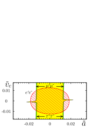
Figure 7: The 95% CL areas in the ($\bar{a},\bar{v}_{e}$) plane for the Bhabha, $e^{+}e^{-}\to\mu^{+}\mu^{-}$, and $e^{+}e^{-}\to\tau^{+}\tau^{-}$ processes.

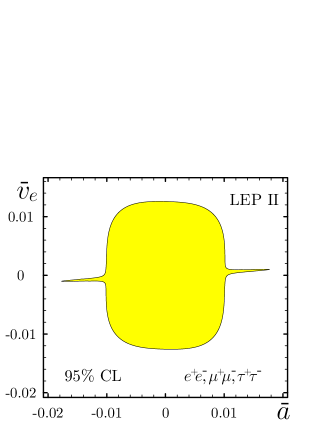
Figure 8: The projection of the 95% CL area onto the ($\bar{a},\bar{v}_{e}$) plane for the combination of the Bhabha, $e^{+}e^{-}\to\mu^{+}\mu^{-}$, and $e^{+}e^{-}\to\tau^{+}\tau^{-}$ processes.

The combination of all the lepton processes is presented in Fig. 8. There is no visible signal beyond the SM. The couplings to the vector and axial-vector electron currents are constrained by the many-parameter fit as $|\bar{v}_{e}|<0.013$, $|\bar{a}|<0.019$ at the 95% CL. If the charge corresponding to the $Z^{\prime}$ interactions is assumed to be of order of the electromagnetic one, then the $Z^{\prime}$ mass should be greater than 0.67 TeV. For the charge of order of the SM $SU(2)_{L}$ coupling constant $m_{Z^{\prime}}\geq 1.4$ TeV. One can see that the constraint is not too severe to exclude the $Z^{\prime}$ searches at the LHC.

Let us compare the obtained results with the one-parameter fits. As one can see, the most precise data of DELPHI and OPAL collaborations are resulted in the Abelian $Z^{\prime}$ hints at one and two standard deviation level, correspondingly. The combined value shows the 2$\sigma$ hint, which corresponds to $0.006\leq|\bar{v}_{e}|\leq 0.020$. On the other hand, our many-parameter fit constrains the $Z^{\prime}$ coupling to the electron vector current as $|\bar{v}_{e}|\leq 0.013$ with no evident signal. Why does the one-parameter fit of the Bhabha process show the 2$\sigma$ CL hint whereas there is no signal in the two-parameter one? Our one-parameter observable accounts mainly for the backward bins. This is in accordance with the kinematic features of the process: the backward bins depend mainly on the vector coupling $\bar{v}^{2}_{e}$, whereas the contributions of other couplings are kinematically suppressed (see Fig. 4). Therefore, the difference of the results can be inspired by the data sets used. To clarify this point, we perform the many-parameter fit with the 113 backward bins ($z\leq 0$), only. The $\chi^{2}$ minimum, $\chi^{2}_{\mathrm{min}}=93.0$, is found in the non-zero point $|\bar{a}|=0.0005$, $\bar{v}_{e}=0.015$. This value of the $Z^{\prime}$ coupling $\bar{v}_{e}$ is in an excellent agreement with the mean value obtained in the one-parameter fit. The 68% confidence area in the ($\bar{a},\bar{v}_{e}$) plane is plotted in Fig. 9. There is a visible hint of the Abelian $Z^{\prime}$ boson. The zero point $\bar{a}=\bar{v}_{e}=0$ (the absence of the $Z^{\prime}$ boson) corresponds to $\chi^{2}=97.7$. It is covered by the confidence area with $1.3\sigma$ CL. Thus, the backward bins show the $1.3\sigma$ hint of the Abelian $Z^{\prime}$ boson in the many-parameter fit. So, the many-parameter fit is less precise than the analysis of the one-parameter observables.

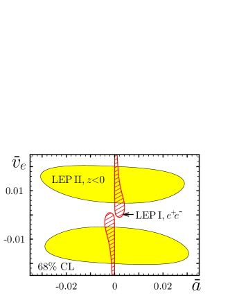
Figure 9: The 68% CL area in the ($\bar{a},\bar{v}_{e}$) plane from the backward bins of the Bhabha process in the LEP2 experiments (the shaded area). The hatched area is the 68% CL area from the LEP 1 data on the Bhabha process.

At LEP1 experiments [24] the $Z$-boson couplings to the vector and axial-vector lepton currents ($g_{V}$, $g_{A}$) were precisely measured. The Bhabha process shows the 1$\sigma$ deviation from the SM values for Higgs boson masses $m_{H}\geq 114$ GeV (see Fig. 7.3 of Ref. [24]). This deviation could be considered as the effect of the $Z$–$Z^{\prime}$ mixing. It is interesting to estimate the bounds on the $Z^{\prime}$ couplings following from these experiments.

Due to the RG relations, the $Z$–$Z^{\prime}$ mixing angle is completely determined by the axial-vector coupling $\bar{a}$. So, the deviations of $g_{V}$, $g_{A}$ from their SM values are governed by the couplings $\bar{a}$ and $\bar{v}_{e}$,

$$g_{V}-g_{V}^{\mathrm{SM}}=-49.06\bar{a}\bar{v}_{e},\quad g_{A}-g_{A}^{\mathrm{SM}}=49.06\bar{a}^{2}.$$ (61)

Let us assume that the total deviation of theory from experiments follows due to the $Z$–$Z^{\prime}$ mixing. This gives an upper bound on the $Z^{\prime}$ couplings. In this way one can estimate whether the $Z^{\prime}$ boson is excluded by the experiments or not.

The 1$\sigma$ CL area for the Bhabha process from Ref. [24] is converted into the ($\bar{a},\bar{v}_{e}$) plane in Fig. 9. The SM values of the couplings correspond to the top quark mass $m_{t}=178$ GeV and the Higgs scalar mass $m_{H}=114$ GeV. As it is seen, the LEP1 data on the Bhabha process is compatible with the Abelian $Z^{\prime}$ existence at the $1\sigma$ CL. The axial-vector coupling is constrained as $|\bar{a}|\leq 0.005$. This bound corresponds to $\bar{a}^{2}\leq 2.5\times 10^{-5}$, which agrees with the one-parameter fits of the LEP2 data for $e^{+}e^{-}\to\mu^{+}\mu^{-},\tau^{+}\tau^{-}$ processes ($\bar{a}^{2}=1.3\pm 3.89\times 10^{-5}$ at 68% CL). On the other hand, the vector coupling constant $\bar{v}_{e}$ is practically unconstrained by the LEP1 experiments.

For the convenience, in Table 4 we collect the summary of the fits of the LEP data in terms of dimensionless contact couplings (7). From the analysis carried out we come to conclusion that, in principle, the LEP experiments were able to detect the $Z^{\prime}$-boson signals if the statistics had been sufficient.

Table 4: The summary of the fits of the LEP data for the dimensionless contact couplings (7).

Data	$\bar{v}^{2}_{e}$	$\bar{a}^{2}$
LEP1
$e^{-}e^{+}$, 68% CL	-	$(1.25\pm 1.25)\times 10^{-5}$
LEP2, one-parameter fits
$e^{-}e^{+}$, 68% CL	$(2.24\pm 0.92)\times 10^{-4}$	-
$\mu\mu$, 68% CL	-	$(3.66^{+4.89}_{-4.86})\times 10^{-5}$
$\mu\mu$,$\tau\tau$, 68% CL	-	$(1.33^{+3.89}_{-3.87})\times 10^{-5}$
LEP2, many-parameter fits
$e^{-}e^{+},\mu\mu,\tau\tau$, 95% CL	$\leq 1.69\times 10^{-4}$	$\leq 3.61\times 10^{-4}$
$e^{-}e^{+}$ backward, 68% CL	$(2.25^{+1.79}_{-2.07})\times 10^{-4}$	$\leq 9.49\times 10^{-4}$

8 $Z^{\prime}$ hints within neural network analysis

Since the actual LEP2 data set is not too large to detect $Z^{\prime}$ boson, one needs in the estimate of its parameters which could be used in future experiments. To determine them in a maximally full way we address to the analysis based on the predictions of the neural networks (for applications in high energy physics see, for example, [25]). The main idea of this approach is to constrain a given data set in such a way that an amount of it is considered as an inessential background and omitted. The remaining data are expected to give a more precise fit of the parameters of interest.

We take into consideration the complete set of the differential cross sections for the Bhabha process accumulated by all the LEP Collaborations and apply the following criteria to restrict the data [26]:

1. As the signal we use the differential cross sections for the Bhabha process accounting for the SM plus $Z^{\prime}$ and calculated at $0.25\times 10^{-4}\leq\bar{v}_{e}^{2}\leq 4\times 10^{-4}$ and $0.25\times 10^{-4}\leq\bar{a}_{e}^{2}\leq 4\times 10^{-4}$.

   Such a choice of parameters is motivated by the results obtained in the previous sections. The cross sections due to the $Z^{\prime}$ exchange diagrams were calculated with the RG relations been taken into consideration.

2. As the background we use the deviations of the experimental differential cross sections from calculated for the SM plus $Z^{\prime}$ ones which are larger than redoubled uncertainties of LEP2 experimental data.

The network trained with these criteria omits the events which correspond to the large deviations from the theoretical cross sections but accounts for the peculiarities proper the $Z^{\prime}$ existence. To construct and train the neural network we used the program MLPFit [27]. The results of the carried out analysis based on the two parametric fit discussed in the previous sections demonstrate the $2\sigma$ CL hint for the $Z^{\prime}$. For the vector coupling the neural network at the $2\sigma$ CL predicts $\bar{v}_{e}^{2}=2.4\pm 1.99\times 10^{-4}$ [26] that is in agreement with the discussed above result derived in the one parametric fit. The obtained values of $\bar{v}_{e}^{2}$ correspond to the value of the mass $m_{Z^{\prime}}=0.53-1.05$ TeV, if the coupling $\tilde{g}$ is of the order of the SM gauge couplings, $g^{2}/(4\pi)\sim 0.01-0.03$. Thus, the carried out analysis demonstrates the hint of $Z^{\prime}$ boson which can be not too heavy. We conclude once again that the data set of the LEP experiments is not sufficient to detect the pronounced signal of this virtual particle.

9 Search for Chiral $Z^{\prime}$ in Bhabha process

Let us turn to the analysis of the Bhabha process with the aim to search for the Chiral $Z^{\prime}$ gauge boson [28]. The Chiral $Z^{\prime}$ interacts with the SM doublets only that can be described by one parameter for each doublet ($\tilde{Y}_{fL}$ and $\tilde{Y}_{\phi}$). It is characterized by the constraints (19)

$$\tilde{Y}_{L,f}=-\tilde{Y}_{fL}\,\sigma_{3},\quad\tilde{Y}_{R,f}=0,\quad\tilde{Y}_{\phi_{i}}=-\tilde{Y}_{\phi}\,\sigma_{3}$$ (62)

where $\sigma_{3}$ is the Pauli matrix.

Remind that in the Bhabha process it is convenient to use the normalized cross-sections (46):

$$\frac{d\tilde{\sigma}}{dz}=\frac{m_{Z}^{2}}{{4\pi}f^{ee}_{2}(z)}\Delta\frac{d\sigma}{dz}=\bar{v}_{e}^{2}+F_{a}\bar{a}_{e}^{2}+F_{av}\bar{a}_{e}\bar{v}_{e}+F_{v\phi}\bar{v}_{e}\bar{\phi}+F_{a\phi}\bar{a}_{e}\bar{\phi}.$$

Since the Chiral $Z^{\prime}$ boson does not interact with the right-handed species, the normalized deviation of the differential cross-section from its SM prediction is determined by two factors, $F_{L}$ and $F_{L\phi}$,

$$\frac{d\tilde{\sigma}}{dz}=\frac{m_{Z}^{2}}{{4\pi}f^{ee}_{2}(z)}\Delta\frac{d\sigma}{dz}=F_{L}\bar{l}_{e}^{2}+F_{L\phi}\bar{l}_{e}\bar{\phi},$$

where we define the dimensionless constants

$$\bar{l}_{f}=\frac{m_{Z}}{\sqrt{4\pi}m_{Z^{\prime}}}\tilde{g}\tilde{Y}_{fL},\quad\bar{\phi}=\frac{m_{Z}}{\sqrt{4\pi}m_{Z^{\prime}}}\tilde{g}\tilde{Y}_{\phi}.$$

The normalization gives us two benefits. First, the obtained factors $F(\sqrt{s},z)$ are finite for all values of the scattering angle $z$. Second, the experimental uncertainties for different bins become equalized that provides the statistical equivalence of different bins. The latter is important for the construction of integrated cross-sections.

The $Z$-$Z^{\prime}$ mixing angle is determined by $\bar{\phi}$ as follows,

$$\theta_{0}\simeq\frac{m_{W}\sin\theta_{W}}{\sqrt{\alpha_{\mathrm{em}}}m_{Z^{\prime}}}\bar{\phi},$$

where $\alpha_{\mathrm{em}}$ is the fine structure constant.

9.1 One-parameter fit for Chiral $Z^{\prime}$

The Chiral $Z^{\prime}$ boson does not interact with the right-handed species. The normalized deviation of the differential cross-section from its SM prediction,

$$d\tilde{\sigma}/dz=F_{L}\bar{l}_{e}^{2}+F_{L\phi}\bar{l}_{e}\bar{\phi},$$

is determined by two finite factors, $F_{L}$ and $F_{L\phi}$, which are shown in Fig. 10.

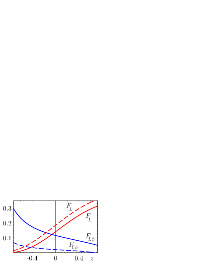
Figure 10: The normalized factors $F_{L}$ and $F_{L\phi}$ describing the Chiral $Z^{\prime}$ effects in the Bhabha process at $\sqrt{s}=200$ GeV (solid lines) and $\sqrt{s}=500$ GeV (dashed lines).

As it is seen, the four-fermion contact coupling $\bar{l}_{e}^{2}$ contributes mainly to the forward scattering angles, whereas the $Z$-$Z^{\prime}$ mixing term affects the backward angles. At the LEP energies they can be of the same order of magnitude. The contribution of the mixing vanishes with the energy growth. We have a possibility to derive the effective experimental constraints on them without any additional restrictions.

First, let us construct a one-parametric observable which is most preferred by the statistical treatment of data. As is clear, it is impossible to separate the couplings $\bar{l}_{e}^{2}$ and $\bar{l}_{e}\bar{\phi}$ in any observable which is an integrated cross-section over some interval of $z$. However, the mixing contribution can be eliminated in the cross-section of the form (which is inspired by the forward-backward asymmetry)

$$\Delta\sigma(z^{*})=\int_{z^{*}}^{z_{\mathrm{max}}}\frac{d\tilde{\sigma}}{dz}\,dz-\int_{-z_{\mathrm{max}}}^{z^{*}}\frac{d\tilde{\sigma}}{dz}\,dz,$$

where the boundary value $z^{*}$ should be chosen to suppress the coefficient at $\bar{l}_{e}\bar{\phi}$. The maximal value of the scattering angle $z_{\mathrm{max}}$ is determined by a particular experiment. In this way we introduce the one-parametric sign-definite observable sensitive to $\bar{l}_{e}^{2}$.

The LEP Collaborations DELPHI and L3 measured the differential cross-sections with $z_{\mathrm{max}}=0.72$ [3, 21]. The set of boundary angles $z^{*}$ as well as the theoretic and experimental values of the observable are collected in Table 5. The other LEP Collaborations – ALEPH and OPAL – used $z_{\mathrm{max}}=0.9$ [2, 20]. The corresponding data are presented in Table 6.

Table 5: The boundary angles $z^{*}$ and the theoretic and experimental values of the observable $\Delta\sigma(z^{*})$ at $z_{\mathrm{max}}=0.72$.

$\sqrt{s}$, GeV $z^{*}$ $\Delta\sigma(z^{*})$ $\Delta\sigma^{\mathrm{ex}}(z^{*})$, DELPHI $\Delta\sigma^{\mathrm{ex}}(z^{*})$, L3 183 -0.245 1742 $\bar{l}_{e}^{2}$ - $-2.38\pm 7.03$ 189 -0.252 1775 $\bar{l}_{e}^{2}$ $-4.28\pm 3.36$ $3.05\pm 3.65$ 192 -0.255 1788 $\bar{l}_{e}^{2}$ $4.57\pm 7.32$ - 196 -0.259 1806 $\bar{l}_{e}^{2}$ $3.77\pm 4.33$ - 200 -0.263 1823 $\bar{l}_{e}^{2}$ $-1.95\pm 4.05$ - 202 -0.265 1831 $\bar{l}_{e}^{2}$ $1.31\pm 5.54$ - 205 -0.267 1843 $\bar{l}_{e}^{2}$ $-4.09\pm 3.89$ - 207 -0.269 1851 $\bar{l}_{e}^{2}$ $0.40\pm 3.33$ -

Table 6: The boundary angles $z^{*}$ and the theoretic and experimental values of the observable $\Delta\sigma(z^{*})$ at $z_{\mathrm{max}}=0.9$.

$\sqrt{s}$, GeV $z^{*}$ $\Delta\sigma(z^{*})$ $\Delta\sigma^{\mathrm{ex}}(z^{*})$, ALEPH $\Delta\sigma^{\mathrm{ex}}(z^{*})$, OPAL 130 -0.217 2017 $\bar{l}_{e}^{2}$ $-12.40\pm 19.24$ $-4.13\pm 29.29$ 136 -0.266 2092 $\bar{l}_{e}^{2}$ $-50.21\pm 16.64$ $-34.18\pm 31.58$ 161 -0.370 2311 $\bar{l}_{e}^{2}$ $-15.90\pm 13.24$ $-14.02\pm 22.32$ 172 -0.400 2398 $\bar{l}_{e}^{2}$ $-12.11\pm 12.50$ $13.71\pm 17.84$ 183 -0.424 2474 $\bar{l}_{e}^{2}$ $-1.51\pm~{}5.18$ $11.04\pm~{}5.57$ 189 -0.435 2512 $\bar{l}_{e}^{2}$ - $-0.63\pm~{}3.28$ 192 -0.441 2531 $\bar{l}_{e}^{2}$ - $-3.48\pm 9.85$ 196 -0.447 2554 $\bar{l}_{e}^{2}$ - $2.96\pm~{}5.09$ 200 -0.454 2577 $\bar{l}_{e}^{2}$ - $0.35\pm~{}4.68$ 202 -0.457 2587 $\bar{l}_{e}^{2}$ - $-2.87\pm~{}9.00$ 205 -0.461 2604 $\bar{l}_{e}^{2}$ - $5.88\pm~{}4.67$ 207 -0.464 2614 $\bar{l}_{e}^{2}$ - $-1.42\pm~{}3.46$

The standard $\chi^{2}$-fit gives the following constraints for the coupling $\bar{l}_{e}^{2}$ at the 68% CL:

$$\mathrm{ALEPH:} \bar{l}_{e}^{2}=-0.00304\pm 0.00176$$

$$\mathrm{DELPHI:} \bar{l}_{e}^{2}=-0.00054\pm 0.00086$$

$$\mathrm{L3:} \bar{l}_{e}^{2}=0.00109\pm 0.00184$$

$$\mathrm{OPAL:} \bar{l}_{e}^{2}=0.00051\pm 0.00064$$

$$\mathrm{Combined:} \bar{l}_{e}^{2}=-0.00004\pm 0.00048$$

Hence it is seen that the most precise data of DELPHI and OPAL collaborations give no signal of the Chiral $Z^{\prime}$ at the 1$\sigma$ CL. The combined value also shows no signal at the 1$\sigma$ CL. From the combined fit the 95% CL bound on the value of $\bar{l}_{e}^{2}$ can be derived, $\bar{l}_{e}^{2}<9\times 10^{-4}$. Supposing the $Z^{\prime}$ coupling constant $\tilde{g}$ to be of the order of the electroweak one, $\tilde{g}\simeq 0.6$, the corresponding $Z^{\prime}$ mass has to be larger than $0.5$ TeV.

9.2 Two parametric fit for Chiral $Z^{\prime}$

A complete two parametric fit of experimental data based directly on the differential cross-sections has been carried out in Ref. [28]. Due to only two independent couplings this fit is efficient. In the fitting the available final data for the differential cross-sections of the Bhabha process were used. The data set consists of 299 bins including the data of ALEPH at 130-183 GeV, DELPHI at 189-207 GeV, L3 at 183-189 GeV, and OPAL at 130-207 GeV [3, 2, 20, 21]. The fitting procedure is similar to that of discussed above for the Abelian $Z^{\prime}$. The results can be summarized as follows.

The parameter space of the Chiral $Z^{\prime}$ is the plane ($\bar{l}_{e}$, $\bar{\phi}$). The minimum of the $\chi^{2}$-function, $\chi^{2}_{\mathrm{min}}=237.29$, is reached at zero value of $\bar{l}_{e}$ ($\simeq 10^{-4}$) and almost independent of the value of $\bar{\phi}$ (the maximal-likelihood values of the couplings). The 95% CL area ($\chi^{2}_{\mathrm{CL}}=5.99$) is shown in Figure 3.

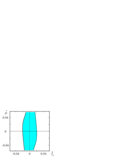
Figure 11: The 95% CL area in $\bar{l}_{e}-\bar{\phi}$ plane. The final data of ALEPH 130-183 GeV, DELPHI GeV 189-207, L3 183-189 GeV, and OPAL 130-207 GeV are combined.

As one can see, the zero point, $\bar{l}_{e}=\bar{\phi}=0$ (the absence of the Chiral $Z^{\prime}$ boson) is inside the confidence area. The value of $\chi^{2}$ in this point (238.62) is indistinguishable from the $\chi^{2}_{\mathrm{min}}$. In other words, the set of experimental data cannot determine the signal of the Chiral $Z^{\prime}$-boson.

As also is seen, the value of $\bar{l}_{e}$ is constrained as $\bar{l}_{e}<0.02$ at the 95% CL. This upper bound is in an agreement with the corresponding result of the one-parameter fit ($\bar{l}_{e}<0.03$). Thus, the $Z^{\prime}$ mass has to be larger than $0.75$ TeV, if the $Z^{\prime}$ coupling constant $\tilde{g}$ is again supposed to be of the order of the electroweak one, $\tilde{g}\simeq 0.6$.

The fit of the differential cross-sections leads to a better accuracy for $\bar{l}_{e}$ than the fit of the integrated cross-sections based on the same data. Without accounting for the model-independent relations between the $Z^{\prime}$ couplings it is impossible to obtain such results.

10 Model independent results and search for $Z^{\prime}$ at the LHC

In this section we discuss all the assumptions giving a possibility to pick out the $Z^{\prime}$ signal and determine its characteristics in a model independent way. We also note the role of the present results for the future LHC and ILC experiments. As it was already stressed, in searching for this particle at the LEP and Tevatron a model dependent analysis was mainly used. The motivation for this was the different number of chiral fermions involved in different models (see, for example, [5]). In this approach, the low bounds on $m_{Z^{\prime}}$ have been estimated and a smallness of the $Z-Z^{\prime}$ mixing was also observed.

On the contrary, in our model independent approach the RG relations between the parameters of the effective low energy Lagrangians have been accounted for that gave a possibility to determine not only the bounds but also the mass and other parameters of the $Z^{\prime}$.

First we note all the assumptions used in our considerations. We analyzed the four-fermion scattering amplitudes of order $\sim m_{Z^{\prime}}^{-2}$ generated by the $Z^{\prime}$ virtual states. The vertices linear in $Z^{\prime}$ were included into the effective low-energy Lagrangian. We also impose a number of natural conditions. The interactions of a renormalizable type are dominant at low energies $\sim m_{W}$. The non-renormalizable interactions generated at high energies due to radiation corrections are suppressed by the inverse heavy mass $\sim 1/m_{Z^{\prime}}$ and neglected. We also assumed that the $SU(2)_{L}\times U(1)_{Y}$ gauge group of the SM is a subgroup of the GUT group. As a consequence, all structure constants connecting two SM gauge bosons with $Z^{\prime}$ are to be zero. Hence, the interactions of gauge fields of the types $Z^{\prime}W^{+}W^{-},Z^{\prime}ZZ$, and other are absent at the tree level. Our effective Lagrangian is also consistent with the absence of the tree-level flavor-changing neutral currents (FCNCs) in the fermion sector. The renormalizable interactions of fermions and scalars are described by the Yukawa Lagrangian (3) that accounts for different possibilities of the Yukawa sector without the tree-level FCNCs. These assumptions are quite general and satisfied in a wide class of $E_{6}$ inspired models.

Within these constraints for the low energy effective Lagrangian the RG correlations have been derived. Correspondingly, the model independent estimates of the mass $m_{Z^{\prime}}$ and other parameters are regulated by the noted requirements. Therefore, the extended underlying model has also to accept them.

In this regard, let us discuss the role of the obtained estimates for the LHC. As it is well known (see, for example, [5, 6]), there are many tools at the LHC for $Z^{\prime}$ identification. But many of them are only applicable if this particle is relatively light. Our results are in favor to this case.

Next important point is the determination of $Z^{\prime}$ couplings to the various SM fermions. As we have shown, the axial-vector couplings of the $Z^{\prime}$ to the SM fermions are universal and proportional to its coupling to the Higgs field. Hence we have obtained an estimate of the $a=a_{f}$ couplings for both leptons and quarks. This is an essential input because experimental analyses for the LHC have mainly concentrated on being able to distinguish models and not on actual couplings. The vector coupling $v_{e}$ was also estimated that, in particular, may help to distinguish the decay of the $Z^{\prime}$ resonance state to $e^{+}e^{-}$ pairs. Since the couplings $a_{e}$ and $v_{e}$ were estimated there is a possibility to distinguish this process from the decay of the $KK$ system. In the literature [6, 29] on searching for the $Z^{\prime}$ it is also mentioned that the determination of the $Z^{\prime}$ couplings to fermions could be fulfilled channel by channel, $a_{e},v_{e},v_{e,b},a_{e,b}$, …. In almost all these considerations the relations between the parameters have not been taken into account. But this is very essential for treating of experimental data and introducing relevant observables to measure.

Other parameter is the $Z-Z^{\prime}$ mixing, which is responsible for different decay processes and the effective interaction vertices generated at the LHC [5, 6]. It is also determined by the axial-vector coupling (see Eq. (21)) and estimated in a model independent way. Remind that in our analysis (in contrast to the approaches of the LEP Collaborations) the mixing was systematically taken into account. Its value is of the same order of magnitude as the parameters that were fitted in experiments. Note also that the existence of other heavy particles with masses $m_{X}\geq m_{Z^{\prime}}$ does not influence the RG relations which are the consequences of the necessary condition for renormalizability. In fact, this condition (the structure of a divergence generated by radiation corrections coincides with that of the tree-level vertex) holds for each renormalizable type interaction.

An important role of the model independent results for searching for $Z^{\prime}$ at the LHC and ILC consists, in particular, in possibility to determine the particle as a virtual state due to a large amount of relevant events. We mentioned already that, in principle, LEP experiments were able to determine it if the statistics was sufficiently large. Experiments at the ILC will increase numerously the data set of interest. In fact, the observables, introduced in sects. 6 and 7 for picking out uniquely $a_{f}^{2}$ and $v_{e}^{2}$ couplings in the leptonic scattering process, are also effective at energies $\sqrt{s}\geq 500$ GeV and could be applied in future experiments at ILC.

Other model independent methods of searching for the $Z^{\prime}$ as a resonance state are proposed in the literature (see Refs. [29, 30, 31]). We do not discuss them here because they take no relations between the parameters into consideration. Besides, the main goal of the present paper is to adduce model independent information about the $Z^{\prime}$ followed from experiments at low energies. Different aspects of $Z^{\prime}$ physics at the LHC are out of the scope of it.

11 Discussion

In this section we collect in a convenient form all the results obtained and make a comparison with other investigations on searching for $Z^{\prime}$ at low energies. In fact, this is a large area to discuss. References to numerous results obtained in either model dependent or model independent approaches can be found in the surveys [5, 6]. Further subdivision can be done into the considerations accounting for any type correlations between the parameters of the low energy effective interactions and that of assuming complete independence of them. Because of a large amount of fitting parameters the latter are less predictable.

Now, for a convenience of readers let us present the results of fits of the $Z^{\prime}$ parameters in terms of the popular notations [4, 5]. The Lagrangian reads

$${\cal L}_{Z\bar{f}f} = \frac{1}{2}Z_{\mu}\bar{f}\gamma^{\mu}\left[(v^{\mathrm{SM}}_{f}+\Delta^{V}_{f})-\gamma^{5}(a^{\mathrm{SM}}_{f}+\Delta^{A}_{f})\right]f,$$

$${\cal L}_{Z^{\prime}\bar{f}f} = \frac{1}{2}Z^{\prime}_{\mu}\bar{f}\gamma^{\mu}\left[(v^{\prime}_{f}-\gamma^{5}a^{\prime}_{f})\right]f,$$ (63)

with the SM values of the $Z$ couplings

$$v^{\mathrm{SM}}_{f}=\frac{e\left(T_{3f}-2Q_{f}\sin^{2}\theta_{W}\right)}{\sin\theta_{W}\cos\theta_{W}},\qquad a^{\mathrm{SM}}_{f}=\frac{e\,T_{3f}}{\sin\theta_{W}\cos\theta_{W}},$$

where $e$ is the positron charge, $Q_{f}$ is the fermion charge in the units of $e$, $T_{3f}=1/2$ for the neutrinos and $u$-type quarks, and $T_{3f}=-1/2$ for the charged leptons and $d$-type quarks.

Table 7: The summary of the fits of the LEP data for the maximum likelihood values of the $Z^{\prime}$ couplings (11) to the SM fermions and of the $Z-Z^{\prime}$ mixing angle $\theta_{0}$. $M=\frac{m_{Z^{\prime}}}{1\,\mathrm{TeV}}$ denotes the unknown value of the $Z^{\prime}$ mass in TeV units.

Data	$|\theta_{0}|$, $\times 10^{-3}$	$|v^{\prime}_{e}|$, $\times 10^{-1}$	$|a^{\prime}_{f}|$, $\times 10^{-1}$	$\Delta^{A}_{e}$, $\times 10^{-3}$
LEP1
$e^{-}e^{+}$	${3.17}{M}^{-1}$	-	$1.38M$	0.437
LEP2, one-parameter fits
$e^{-}e^{+}$	-	$5.83M$	-	-
$\mu^{-}\mu^{+}$	$5.42{M}^{-1}$	-	$2.36M$	1.278
$\mu^{-}\mu^{+},\tau^{-}\tau^{+}$	$3.27{M}^{-1}$	-	$1.42M$	0.464
LEP2, many-parameter fits
$e^{-}e^{+}$, $z<0$	-	$5.84M$	-	-

Table 8: The summary of the fits of the LEP data for the confidence intervals for the $Z^{\prime}$ couplings (11) to the SM fermions and for the $Z-Z^{\prime}$ mixing angle $\theta_{0}$. $M=\frac{m_{Z^{\prime}}}{1\,\mathrm{TeV}}$ denotes the unknown value of the $Z^{\prime}$ mass in TeV units.

Data	CL	$|\theta_{0}|$, $\times 10^{-3}$	$|v^{\prime}_{e}|$, $\times 10^{-1}$	$|a^{\prime}_{f}|$, $\times 10^{-1}$	$\Delta^{A}_{e}$, $\times 10^{-3}$
LEP1
$e^{-}e^{+}$	68%	$(0;4.48){M}^{-1}$	-	$(0;1.95)M$	$(0;0.873)$
LEP2, one-parameter fits
$e^{-}e^{+}$	95%	-	$(2.46;7.87)M$	-	-
$\mu^{-}\mu^{+}$	95%	$(0;10.39){M}^{-1}$	-	$(0;4.52)M$	$(0;4.694)$
$\mu^{-}\mu^{+}$,
$\tau^{-}\tau^{+}$	95%	$(0;8.64){M}^{-1}$	-	$(0;3.75)M$	$(0;3.244)$
LEP2, many-parameter fits
$e^{-}e^{+}$,
$\mu^{-}\mu^{+}$,	95%	$(0;17.03){M}^{-1}$	$(0;5.06)M$	$(0;7.40)M$	$(0;12.607)$
$\tau^{-}\tau^{+}$
$e^{-}e^{+}$,
$z<0$	68%	$(0;27.61){M}^{-1}$	$(1.68;7.83)M$	$(0;12.00)M$	$(0;33.1288)$

The results of the fits of the $Z^{\prime}$ couplings to the SM leptons obtained from the analysis of the LEP experiments are adduced in the Tables 7-8 and Fig. 12. Remind that due to the universality of the axial-vector coupling $a_{f}$ the same estimates take also place for quarks. First of all, one parameter fits of LEP experiments as well as the many-parameter fit for the $e^{+}e^{-}$ backward bins show the hints of the $Z^{\prime}$ boson at the 1-2$\sigma$ CL. Due to this fact, the fits allow to determine the maximum likelihood values of $Z^{\prime}$ parameters. In spite of uncertainties, these values can be used as a guiding line for the estimation of possible $Z^{\prime}$ effects in the LHC experiments. The maximum likelihood values are given in Table 7. As is seen, different fits and processes lead to the comparable values of the $Z^{\prime}$ parameters.

In Table 8 we present the confidence intervals for the fitted parameters. With this Table one is able to estimate the uncertainty of the $Z^{\prime}$ couplings as well as the lower bounds on the parameters.

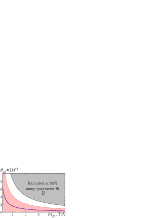
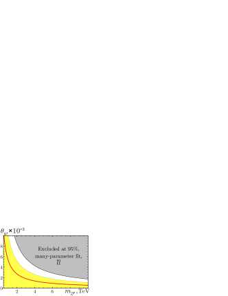
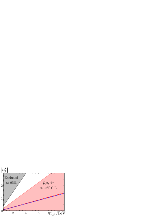
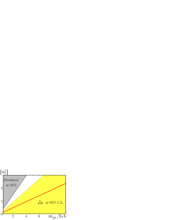
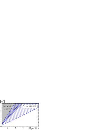
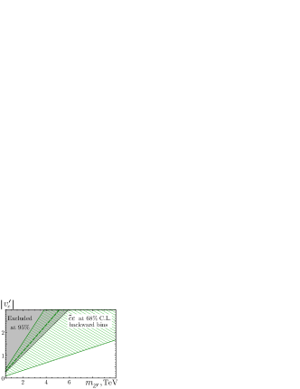
Figure 12: The maximum likelihood values and the confidence intervals for the $Z-Z^{\prime}$ mixing angle ($\theta_{0}$), the vector coupling to electron current ($v^{\prime}_{e}$), and the axial-vector couplings to the SM fermions ($a^{\prime}_{f}$) by the LEP 2 data. The values excluded at 95% CL by the many-parameter fit of $e^{+}e^{-}\to l^{+}l^{-}$ are shown in gray. The results of fits based on the one-parameter observables are shown in pink for $e^{+}e^{-}\to\mu^{+}\mu^{-},\tau^{+}\tau^{-}$ (with the maximum likelihood value as the dashed red line), in yellow for $e^{+}e^{-}\to\mu^{+}\mu^{-}$ (with the maximum likelihood value as the solid red line), and in blue for $e^{+}e^{-}\to e^{+}e^{-}$ (with the maximum likelihood value as the dashed blue line). The maximum likelihood values and the 1$\sigma$ CL area for the many-parameter fit of backward bins of $e^{+}e^{-}\to e^{+}e^{-}$ are also shown in green. The blue dotted lines correspond to the maximum likelihood values obtained from the LEP1 data.

In Fig. 12 the maximum likelihood values and the CL intervals are drawn for the different values of the $Z^{\prime}$ mass. All the plots exploit the same color scheme. The values excluded at 95% CL by the many-parameter fit of all the LEP2 leptonic processes $e^{+}e^{-}\to l^{+}l^{-}$ are shown in gray. The 95% confidence intervals from the one-parameter fit of LEP2 $e^{+}e^{-}\to\mu^{+}\mu^{-},\tau^{+}\tau^{-}$ are drawn in pink with the maximum likelihood values as the dashed red line. The corresponding results with taking into account the $\mu^{+}\mu^{-}$ process only are shown in yellow with solid red line for the maximum likelihood values. The maximum likelihood values from the LEP1 experiments are represented as dotted blue line. The 95% confidence interval from the one-parameter fit of the LEP2 Bhabha scattering is shown as the blue crosshatched region with the maximum likelihood values as the dashed blue line. Finally, the 68% confidence interval and the maximum likelihood values from the many-parameter fit of the backward bins of LEP2 Bhabha scattering are shown in green.

Now we compare the above results with the ones of other fits accounting for the $Z^{\prime}$ presence. As it was mentioned in Introduction, LEP collaborations have determined the model dependent low bounds on the $Z^{\prime}$ mass which vary in a wide energy interval dependently on a model. The same has also been done for Tevatron experiments. The modern low bound is $m_{Z^{\prime}}\geq 850$ GeV. It is also well known that though almost all the present day data are described by the SM [1, 2, 3, 24], the overall fit to the standard model is not very good. In Ref. [7] it was showed that the large difference in $\sin^{2}\theta^{\mathrm{lept}}_{\mathrm{eff}}$ from the forward-backward asymmetry $A^{b}_{fb}$ of the bottom quarks and the measurements from the SLAC SLD experiment can be explained for physically reasonable Higgs boson mass if one allows for one or more extra $U(1)$ fields, that is $Z^{\prime}$. A specific model to describe $Z^{\prime}$ physics of interest was proposed which introduces two type couplings to the hyper charge $Y$ and to the baryon-minus-lepton number $B-L$. Within this model by using a number of precision measurements from LEP1, LEP2, SLD and Tevatron experiments the parameters $a_{Y}$ and $a_{B-L}$ of the model were fitted. The presence of $Z^{\prime}$ was not excluded at 68% CL. The value of $a_{Y}$ was estimated to be of the same order of magnitude as in our analysis and is comparable with values of other parameters detected in the LEP experiments. The erroneous claim that $a_{Y}$ is two order less then the value derived from our Table 4 is, probably, a consequence of some missed factors. The upper limit on the mass was also obtained $m_{Z^{\prime}}\leq 2.6$ TeV .

These two analyzes are different but complementary. A common feature of them is an accounting for the $Z^{\prime}$ gauge boson as a necessary element of the data fits. The results are in accordance at 68-95% CL with the existence of the not heavy $Z^{\prime}$ which has a good chance to be discovered at Tevatron and/or LHC.

Appendix. RG relations in a theory with different mass scales

In this Appendix we are going to investigate the Yukawa model with a heavy scalar field $\chi$ and a light scalar field $\varphi$ [32]. The goals of our investigation are two fold: 1) to derive the one-loop RG relation for the four-fermion scattering amplitude in the decoupling region and 2) to find out the possibility of reducing this relation in the equation for vertex describing the scattering of light particles on the external field when the mixing between heavy and light virtual states takes place.

The Lagrangian of the model reads

$${\cal L} = \frac{1}{2}{\left(\partial_{\mu}\varphi\right)}^{2}-\frac{m^{2}}{2}{\varphi}^{2}-\lambda{\varphi}^{4}+\frac{1}{2}{\left(\partial_{\mu}\chi\right)}^{2}-\frac{{\Lambda}^{2}}{2}{\chi}^{2}-\xi{\chi}^{4}$$ (64)

$$+\rho{\varphi}^{2}{\chi}^{2}+{\bar{\psi}}\left(i\partial_{\mu}\gamma_{\mu}-M-G_{\varphi}\varphi-G_{\chi}\chi\right)\psi,$$

where $\psi$ is a Dirac spinor field, and $\Lambda\gg m,M$.

Consider the four-fermion scattering $\bar{\psi}\psi\to\bar{\psi}\psi$. The $S$-matrix element at the one-loop level is given by

$${\hat{S}} = -\frac{i}{2}\int\frac{dp_{1}}{{\left(2\pi\right)}^{4}}\ldots\frac{dp_{4}}{{\left(2\pi\right)}^{4}}{\left(2\pi\right)}^{4}\delta\left(p_{1}+...+p_{4}\right)\left[S_{\mathrm{1PR}}+S_{\mathrm{box}}\right],$$

$$S_{\mathrm{1PR}} = \sum\limits_{{\phi}_{1},{\phi}_{2}=\varphi,\chi}G_{{\phi}_{1}}G_{{\phi}_{2}}\left(\frac{{\delta}_{{\phi}_{1}{\phi}_{2}}}{s-m^{2}_{{\phi}_{1}}}+\frac{\Pi_{\phi_{1}\phi_{2}}(s)}{(s-m^{2}_{\phi_{1}})(s-m^{2}_{\phi_{2}})}\right)$$ (65)

$$\times{\bar{\psi}}\left(p_{4}\right)\left[1+\Gamma\left(p_{3},-p_{4}-p_{3}\right)\right]\psi\left(p_{3}\right)$$

$$\times{\bar{\psi}}\left(p_{1}\right)\left[1+\Gamma\left(p_{2},-p_{1}-p_{2}\right)\right]\psi\left(p_{2}\right),$$

where $s={\left(p_{1}+p_{2}\right)}^{2}$, $S_{\mathrm{1PR}}$ is the contribution from the one-particle reducible diagrams shown in Figs. 13-14, and $S_{\mathrm{box}}$ is the contribution from box diagrams.

Figure 13: Tree level contribution to the four-fermion amplitude.

Figure 14: The one-loop level contribution to the one-particle reducible four-fermion amplitude.

The one-loop polarization operator of scalar fields ${\Pi}_{{\phi}_{1}{\phi}_{2}}$ and the one-loop vertex function $\Gamma$ are related to the Green functions as

$$D_{{\phi}_{1}{\phi}_{2}}\left(s\right) = \frac{{\delta}_{{\phi}_{1}{\phi}_{2}}}{s-m^{2}_{{\phi}_{1}}}+\frac{1}{s-m^{2}_{{\phi}_{1}}}{\Pi}_{{\phi}_{1}{\phi}_{2}}\left(s\right)\frac{1}{s-m^{2}_{{\phi}_{2}}},$$

$$G_{\phi\phi\psi}\left(p,q\right) = -\sum\limits_{{\phi}_{1}}G_{{\phi}_{1}}D_{{\phi}_{1}\phi}\left(q^{2}\right)S_{\psi}\left(p\right)\left(1+\Gamma\left(p,q\right)\right)S_{\psi}\left(-p-q\right),$$ (66)

where $S_{\psi}$ is the spinor propagator in the momentum representation.

Renormalization of the model

The renormalized fields, masses and charges are defined as follows

$$\left(\begin{array}[]{c}\varphi\\ \chi\end{array}\right)=Z_{\phi}^{-1/2}\left(\begin{array}[]{c}\varphi_{0}\\ \chi_{0}\end{array}\right),\qquad\left(\begin{array}[]{c}G_{\varphi}\\ G_{\chi}\end{array}\right)=Z_{G}^{-1}\left(\begin{array}[]{c}G_{\varphi,0}\\ G_{\chi,0}\end{array}\right),$$ (75)

$$\psi=Z_{\psi}^{-1/2}\psi_{0},\qquad M^{2}=M_{0}^{2}-\delta M^{2},$$

$$m^{2}=m_{0}^{2}-\delta m^{2},\qquad\Lambda^{2}=\Lambda_{0}^{2}-\delta\Lambda^{2},$$ (76)

where subscript 0 marks the corresponding bare quantities.

Using the dimensional regularization (the dimension of the momentum space is $D=4-\varepsilon$) and the $\overline{\mathrm{MS}}$ renormalization scheme one can compute the renormalization constants

$$Z_{\psi} = 1-\frac{1}{16\pi^{2}\varepsilon}\left(G_{\varphi}^{2}+G_{\chi}^{2}\right),$$

$$\delta M^{2} = \frac{3}{8\pi^{2}\varepsilon}\left(G_{\varphi}^{2}+G_{\chi}^{2}\right)M^{2},$$

$$Z_{\phi}^{1/2} = 1-\frac{1}{8\pi^{2}\varepsilon}\left(\begin{array}[]{cc}G_{\varphi}^{2}&2G_{\varphi}G_{\chi}\frac{\Lambda^{2}-6M^{2}}{\Lambda^{2}-m^{2}}\\ -2G_{\varphi}G_{\chi}\frac{m^{2}-6M^{2}}{\Lambda^{2}-m^{2}}&G_{\chi}^{2}\end{array}\right),$$ (79)

$$\delta m^{2} = \frac{1}{4\pi^{2}\varepsilon}\left[\left(G_{\varphi}^{2}+6\lambda\right)m^{2}-6G_{\varphi}^{2}M^{2}-\rho\Lambda^{2}\right],$$

$$\delta\Lambda^{2} = \frac{1}{4\pi^{2}\varepsilon}\left[\left(G_{\chi}^{2}+6\xi\right)\Lambda^{2}-6G_{\chi}^{2}M^{2}-\rho m^{2}\right],$$

$$Z_{G}^{-1} = \left[1-\frac{3}{16\pi^{2}\varepsilon}\left(G_{\varphi}^{2}+G_{\chi}^{2}\right)\right]{\left(Z_{\phi}^{1/2}\right)}^{\mathrm{T}}.$$ (80)

From Eq. (Renormalization of the model) we obtain the appropriate $\beta$ and $\gamma$ functions at the one-loop level:

$$\beta_{\varphi} = \frac{dG_{\varphi}}{d\log\kappa}=\frac{G_{\varphi}}{16\pi^{2}}\left(5G_{\varphi}^{2}+3G_{\chi}^{2}-4\frac{m^{2}-6M^{2}}{\Lambda^{2}-m^{2}}G_{\chi}^{2}\right),$$

$$\beta_{\chi} = \frac{dG_{\chi}}{d\log\kappa}=\frac{G_{\chi}}{16\pi^{2}}\left(5G_{\chi}^{2}+3G_{\varphi}^{2}+4\frac{\Lambda^{2}-6M^{2}}{\Lambda^{2}-m^{2}}G_{\varphi}^{2}\right),$$

$$\gamma_{m} = -\frac{d\log m^{2}}{d\log\kappa}=-\frac{1}{4\pi^{2}}\left(G_{\varphi}^{2}\frac{m^{2}-6M^{2}}{m^{2}}+6\lambda-\rho\frac{\Lambda^{2}}{m^{2}}\right),$$

$$\gamma_{\Lambda} = -\frac{d\log\Lambda^{2}}{d\log\kappa}=-\frac{1}{4\pi^{2}}\left(G_{\chi}^{2}\frac{\Lambda^{2}-6M^{2}}{\Lambda^{2}}+6\xi-\rho\frac{m^{2}}{\Lambda^{2}}\right),$$

$$\gamma_{\psi} = -\frac{d\log\psi}{d\log\kappa}=\frac{1}{32\pi^{2}}\left(G_{\varphi}^{2}+G_{\chi}^{2}\right).$$ (81)

Then, the $S$-matrix element can be expressed in terms of the renormalized quantities. The contribution from the one-particle reducible diagrams becomes

$$S_{\mathrm{1PR}} = \sum\limits_{\phi_{1},\phi_{2}}G_{\phi_{1}}G_{\phi_{2}}\left(\frac{\delta_{\phi_{1}\phi_{2}}}{s-m^{2}_{\phi_{1}}}+\frac{\Pi_{\phi_{1}\phi_{2}}^{\mathrm{(fin)}}(s)}{(s-m^{2}_{\phi_{1}})(s-m^{2}_{\phi_{2}})}\right)$$ (82)

$$\times\bar{\psi}(p_{4})\left[1+\Gamma^{\mathrm{(fin)}}\left(p_{3},-p_{4}-p_{3}\right)\right]\psi(p_{3})$$

$$\times\bar{\psi}(p_{1})\left[1+\Gamma^{\mathrm{(fin)}}\left(p_{2},-p_{1}-p_{2}\right)\right]\psi(p_{2}),$$

where the functions $\Pi_{\phi_{1}\phi_{2}}^{\mathrm{(fin)}}$ and $\Gamma^{\mathrm{(fin)}}$ are the expressions $\Pi_{\phi_{1}\phi_{2}}$ and $\Gamma$ without the terms proportional to $1/\varepsilon$. Since the quantity $S_{\mathrm{box}}$ is finite, the renormalization leaves it without changes.

Introducing the RG operator at the one-loop level [18]

$${\cal D} = \frac{d}{d\log\kappa}=\frac{\partial}{\partial\log\kappa}+{\cal D}^{(1)}=\frac{\partial}{\partial\log\kappa}$$ (83)

$$+\sum\limits_{\phi}\beta_{\phi}\frac{\partial}{\partial G_{\phi}}-\gamma_{m}\frac{\partial}{\partial\log m^{2}}-\gamma_{\Lambda}\frac{\partial}{\partial\log\Lambda^{2}}-\gamma_{\psi}\frac{\partial}{\partial\log\psi}$$

we determine that the following relation holds for the $S$-matrix element

$${\cal D}\left(S_{\mathrm{1PR}}+S_{\mathrm{box}}\right)=\frac{\partial S_{\mathrm{1PR}}^{(1)}}{\partial\log\kappa}+{\cal D}^{(1)}S_{\mathrm{1PR}}^{(0)}=0,$$ (84)

where the $S_{\mathrm{1PR}}^{(0)}$ and the $S_{\mathrm{1PR}}^{(1)}$ are the contributions to the $S_{\mathrm{1PR}}$ at the tree level and at the one-loop level, respectively:

$$S_{\mathrm{1PR}}^{(0)}=\left(\frac{G_{\varphi}^{2}}{s-m^{2}}+\frac{G_{\chi}^{2}}{s-\Lambda^{2}}\right)\bar{\psi}\psi\times\bar{\psi}\psi,$$ (85)

$$\frac{\partial S_{\mathrm{1PR}}^{(1)}}{\partial\log\kappa} = \frac{\bar{\psi}\psi\times\bar{\psi}\psi}{4\pi^{2}}\left[-\left(G_{\varphi}^{2}+G_{\chi}^{2}\right)\left(\frac{G_{\varphi}^{2}}{s-m^{2}}+\frac{G_{\chi}^{2}}{s-\Lambda^{2}}\right)\right.$$ (86)

$$+\frac{G_{\varphi}^{2}\left(\rho\Lambda^{2}-6\lambda m^{2}+G_{\varphi}^{2}\left(6M^{2}-s\right)\right)}{\left(s-m^{2}\right)^{2}}$$

$$+\frac{2G_{\varphi}^{2}G_{\chi}^{2}\left(6M^{2}-s\right)}{\left(s-m^{2}\right)\left(s-\Lambda^{2}\right)}$$

$$\left.+\frac{G_{\chi}^{2}\left(\rho m^{2}-6\xi\Lambda^{2}+G_{\chi}^{2}\left(6M^{2}-s\right)\right)}{\left(s-\Lambda^{2}\right)^{2}}\right].$$

The first term in Eq. (86) is originated from the one-loop correction to the fermion-scalar vertex. The rest terms are connected with the polarization operator of scalars. The third term describes the one-loop mixing between the scalar fields. It is canceled in the RG relation (84) by the mass-dependent terms in the $\beta$ functions produced by the non-diagonal elements in $Z_{\phi}$.

Eq. (84) is the consequence of the renormalizability of the model. It insures the leading logarithm terms of the one-loop $S$-matrix element to reproduce the appropriate tree-level structure. In contrast to the familiar treatment we are not going to improve scattering amplitudes by solving Eq. (84). We will use it as an algebraic identity implemented in the renormalizable theory. Naturally if one knows the explicit couplings expressed in terms of the basic set of parameters of the model, this RG relation is trivially fulfilled. But the situation changes when the couplings are represented by unknown arbitrary parameters. In this case the RG relations are the algebraic equations dependent on these parameters and appropriate $\beta$ and $\gamma$ functions. In the presence of a symmetry the number of $\beta$ and $\gamma$ functions is less than the number of RG relations. So, one has non trivial system of equations relating the unknown couplings. For example, such a scenario is realized for the gauge coupling. Although the considered simple model has no gauge couplings, we are able to demonstrate the general procedure of deriving the RG relations.

Decoupling of the heavy field

At energies $s\ll\Lambda^{2}$ the heavy scalar field $\chi$ is decoupled. This means, that the four-fermion scattering amplitude is described by the model with no heavy field $\chi$ plus terms of the order $s/\Lambda^{2}$. At the tree level, this is the obvious consequence of the expansion of the heavy scalar propagator

$$\frac{1}{s-\Lambda^{2}}\to-\frac{1}{\Lambda^{2}}\left[1+O\left(\frac{s}{\Lambda^{2}}\right)\right],$$ (87)

which is resulted in the effective contact four-fermion interaction in Eq. (85)

$${\cal L}_{\mathrm{eff}}=-\alpha\,\bar{\psi}\psi\times\bar{\psi}\psi,\quad\alpha=\frac{G_{\chi}^{2}}{\Lambda^{2}}.$$ (88)

So, the tree level contribution to the scattering amplitude becomes

$$S_{\mathrm{1PR}}^{(0)}=\left[\frac{G_{\varphi}^{2}}{s-m^{2}}-\alpha+O\left(\frac{s}{\Lambda^{4}}\right)\right]\bar{\psi}\psi\times\bar{\psi}\psi,$$ (89)

and the lowest order effects of the heavy scalar in the decoupling region are described by the parameter $\alpha$, only.

Decoupling of heavy particles is present also at the level of radiative corrections. The radiative corrections are generally described by various loop integrals in the momentum space (the Passarino–Veltman functions). Considering a Passarino–Veltman function with at least one heavy mass $Lambda$ inside loop in the low-energy limit, one can see the following asymptotic behavior: the function splits into 1) possible energy-independent divergent part (including also $\log\Lambda$) and 2) energy-dependent finite part which can be expanded by inverse powers of $\Lambda$ and vanishes at the small energies. The important property is that the $\log\Lambda$-term in the divergent part reproduces the logarithm of the cut-off scale. So, such a potentially large term has to be automatically absorbed by the renormalization at low energies and leads to no observable effects. However, if the renormalization is actually performed at high energies (as in the $\overline{\mathrm{MS}}$ renormalization scheme) the potentially large $\log\Lambda$-terms should be re-summed manually by the redefinition of the physical couplings and masses at the scale $\Lambda$.

What is the form of the RG relations in the limit of large $\Lambda$? The method of constructing the RG equation in the decoupling region was proposed in [18]. It introduces the redefinition of the parameters of the model allowing to remove all the heavy particle loop contributions to Eq. (86). Let us define a new set of fields, charges and masses $\tilde{\psi}$, $\tilde{G}_{\varphi}$, $\tilde{G}_{\chi}$, $\tilde{\Lambda}$, $\tilde{m}$, $\tilde{M}$

$$G_{\varphi}^{2} = \tilde{G}_{\varphi}^{2}\left(1+\frac{3\tilde{G}_{\chi}^{2}}{16\pi^{2}}\log\frac{\kappa^{2}}{\tilde{\Lambda}^{2}}+\ldots\right),$$

$$G_{\chi}^{2} = \tilde{G}_{\chi}^{2}\left(1+\frac{3\tilde{G}_{\chi}^{2}}{16\pi^{2}}\log\frac{\kappa^{2}}{\tilde{\Lambda}^{2}}+\ldots\right),$$

$$m^{2} = \tilde{m}^{2}\left(1-\frac{\tilde{\rho}}{8\pi^{2}}\frac{\tilde{\Lambda}^{2}}{\tilde{m}^{2}}\log\frac{\kappa^{2}}{\tilde{\Lambda}^{2}}+\ldots\right),$$

$$\Lambda^{2} = \tilde{\Lambda}^{2}\left(1+\frac{3\tilde{\xi}}{4\pi^{2}}\log\frac{\kappa^{2}}{\tilde{\Lambda}^{2}}+\ldots\right),$$

$$\psi = \tilde{\psi}\left(1-\frac{\tilde{G}_{\chi}^{2}}{64\pi^{2}}\log\frac{\kappa^{2}}{\tilde{\Lambda}^{2}}+\ldots\right),$$ (90)

where dots stand for the higher powers of $\log\Lambda$ responsible for the decoupling at higher loop orders.

The differential operator (83) ban be rewritten in terms of these new low-energy parameters:

$${\cal D} = \frac{\partial}{\partial\log\kappa}+{\tilde{\cal D}}^{(1)}=\frac{\partial}{\partial\log\kappa}+\sum\limits_{\phi}\tilde{\beta}_{\phi}\frac{\partial}{\partial\tilde{G}_{\phi}}$$ (91)

$$-\tilde{\gamma}_{m}\frac{\partial}{\partial\log\tilde{m}^{2}}-\tilde{\gamma}_{\Lambda}\frac{\partial}{\partial\log\tilde{\Lambda}^{2}}-\tilde{\gamma}_{\psi}\frac{\partial}{\partial\log\tilde{\psi}}$$

where $\tilde{\beta}$ and $\tilde{\gamma}$ functions are obtained from the one-loop relations (Renormalization of the model) and (Decoupling of the heavy field)

$$\tilde{\beta}_{\varphi}=\frac{1}{16\pi^{2}}\left(5\tilde{G}_{\varphi}^{3}-4\frac{\tilde{m}^{2}-6\tilde{M}^{2}}{\tilde{\Lambda}^{2}-\tilde{m}^{2}}\tilde{G}_{\varphi}\tilde{G}_{\chi}^{2}\right),$$

$$\tilde{\beta}_{\chi}=\frac{1}{16\pi^{2}}\left(2\tilde{G}_{\chi}^{3}+\left(3+4\frac{\tilde{\Lambda}^{2}-6\tilde{M}^{2}}{\tilde{\Lambda}^{2}-\tilde{m}^{2}}\right)\tilde{G}_{\chi}\tilde{G}_{\varphi}^{2}\right),$$

$$\tilde{\gamma}_{m}=-\frac{1}{4\pi^{2}}\left(\tilde{G}_{\varphi}^{2}\frac{\tilde{m}^{2}-6\tilde{M}^{2}}{\tilde{m}^{2}}+6\tilde{\lambda}\right),$$

$$\tilde{\gamma}_{\Lambda}=-\frac{1}{4\pi^{2}}\left(\tilde{G}_{\chi}^{2}\left(1-6\frac{\tilde{M}^{2}}{\tilde{\Lambda}^{2}}\right)-\tilde{\rho}\frac{\tilde{m}^{2}}{\tilde{\Lambda}^{2}}\right),$$

$$\tilde{\gamma}_{\psi}=\frac{1}{32\pi^{2}}\tilde{G}_{\varphi}^{2}.$$ (92)

Hence, one immediately notices that $\tilde{\beta}$ and $\tilde{\gamma}$ functions contain only the light particle loop contributions, and all the heavy particle loop terms are completely removed from them. The $S$-matrix element expressed in terms of new parameters satisfies the following RG relation

$${\cal D}\left(S_{\mathrm{1PR}}+S_{\mathrm{box}}\right)=\frac{\partial\tilde{S}_{\mathrm{1PR}}^{(1)}}{\partial\log\kappa}+{\tilde{\cal D}}^{(1)}\tilde{S}_{\mathrm{1PR}}^{(0)}=0,$$ (93)

$$\tilde{S}_{\mathrm{1PR}}^{(0)}=\left(\frac{\tilde{G}_{\varphi}^{2}}{s-\tilde{m}^{2}}-\tilde{\alpha}+O\left(\frac{s^{2}}{\tilde{\Lambda}^{4}}\right)\right){\bar{\tilde{\psi}}}\tilde{\psi}\times{\bar{\tilde{\psi}}}\tilde{\psi},$$ (94)

$$\frac{\partial\tilde{S}_{\mathrm{1PR}}^{(1)}}{\partial\log\kappa} = \frac{{\bar{\tilde{\psi}}}\tilde{\psi}\times{\bar{\tilde{\psi}}}\tilde{\psi}}{4\pi^{2}}\left(-\frac{\tilde{G}_{\varphi}^{4}}{s-\tilde{m}^{2}}\right.$$ (95)

$$\left.+\frac{\tilde{G}_{\varphi}^{2}\left(-6\tilde{\lambda}\tilde{m}^{2}+\tilde{G}_{\varphi}^{2}\left(6\tilde{M}^{2}-s\right)\right)}{\left(s-\tilde{m}^{2}\right)^{2}}+\tilde{\alpha}\tilde{G}_{\varphi}^{2}\right.$$

$$\left.-\frac{2\tilde{G}_{\varphi}^{2}\tilde{\alpha}\left(6\tilde{M}^{2}-s\right)}{s-\tilde{m}^{2}}+O\left(\frac{s^{2}}{\tilde{\Lambda}^{4}}\right)\right),$$

where $\tilde{\alpha}=\tilde{G}_{\chi}^{2}/\tilde{\Lambda}^{2}$ is the redefined effective four-fermion coupling. As one can see, Eq. (95) includes all the terms of Eq. (86) except for the heavy particle loop contributions. It depends on the low energy quantities $\tilde{\psi}$, $\tilde{G}_{\varphi}$, $\tilde{\alpha}$, $\tilde{\lambda}$, $\tilde{m}$, $\tilde{M}$. The first and the second terms in Eq. (95) are just the one-loop amplitude calculated within the model with no heavy particles. The third and the fourth terms describe the light particle loop correction to the effective four-fermion coupling and the mixing of heavy and light virtual fields.

Elimination of the one-loop scalar field mixing

Due to the mixing term it is impossible to split the RG relation (93) for the $S$-matrix element into the one for vertices. Hence, we are not able to consider Eq. (93) in the framework of the scattering of light particles on an external field induced by the heavy virtual scalar. But this is an important step in deriving the RG relation for EL parameters. Fortunately, there is a simple procedure allowing to avoid the mixing in Eq. (95). The way is to incorporate the diagonalization of the leading logarithm terms of the scalar polarization operator into the redefinition of the $\tilde{\varphi}$, $\tilde{\chi}$, $\tilde{G}_{\varphi}$, $\tilde{G}_{\chi}$:

$$\left(\begin{array}[]{c}\varphi\\ \chi\end{array}\right) = {\zeta}^{1/2}\left(\begin{array}[]{c}{\tilde{\varphi}}\\ {\tilde{\chi}}\end{array}\right),$$ (100)

$$\left(\begin{array}[]{c}G_{\varphi}\\ G_{\chi}\end{array}\right) = \left[1+\frac{3\tilde{G}_{\chi}^{2}}{32\pi^{2}}\log\frac{\kappa^{2}}{\tilde{\Lambda}^{2}}\right]\left(\zeta^{-1/2}\right)^{\mathrm{T}}\left(\begin{array}[]{c}\tilde{G}_{\varphi}\\ \tilde{G}_{\chi}\end{array}\right),$$ (105)

$$\zeta^{1/2} = 1-\frac{\tilde{G}_{\varphi}\tilde{G}_{\chi}}{8\pi^{2}\left(\tilde{\Lambda}^{2}-\tilde{m}^{2}\right)}\log\frac{\kappa^{2}}{\tilde{\Lambda}^{2}}\left(\begin{array}[]{cc}0&\tilde{\Lambda}^{2}-6\tilde{M}^{2}\\ -\tilde{m}^{2}-6\tilde{M}^{2}&0\end{array}\right).$$ (108)

The appropriate $\tilde{\beta}$ functions

$$\tilde{\beta}_{\varphi}=\frac{5\tilde{G}_{\varphi}^{3}}{16\pi^{2}},\quad\tilde{\beta}_{\chi}=\frac{1}{16\pi^{2}}\left(2\tilde{G}_{\chi}^{3}+3\tilde{G}_{\chi}\tilde{G}_{\varphi}^{2}\right)$$ (109)

contain no terms connected with mixing between light and heavy scalars. So, the fourth term in Eq. (95) is removed, and the RG relation for the $S$-matrix element becomes

$${\cal D}\left(S_{\mathrm{1PR}}+S_{\mathrm{box}}\right)=\frac{\partial\tilde{S}_{\mathrm{1PR}}^{(1)}}{\partial\log\kappa}+{\tilde{\cal D}}^{(1)}\tilde{S}_{\mathrm{1PR}}^{(0)}=0,$$ (110)

$$\tilde{S}_{\mathrm{1PR}}^{(0)}=\left(\frac{\tilde{G}_{\varphi}^{2}}{s-\tilde{m}^{2}}-\tilde{\alpha}+O\left(\frac{s^{2}}{\tilde{\Lambda}^{4}}\right)\right)\bar{\tilde{\psi}}\tilde{\psi}\times\bar{\tilde{\psi}}\tilde{\psi},$$ (111)

$$\frac{\partial{\tilde{S}}_{\mathrm{1PR}}^{(1)}}{\partial\log\kappa} = \frac{\bar{\tilde{\psi}}\tilde{\psi}\times\bar{\tilde{\psi}}\tilde{\psi}}{4\pi^{2}}\left(-\frac{\tilde{G}_{\varphi}^{4}}{s-\tilde{m}^{2}}\right.$$ (112)

$$\left.+\frac{\tilde{G}_{\varphi}^{2}\left(-6\tilde{\lambda}\tilde{m}^{2}+\tilde{G}_{\varphi}^{2}\left(6\tilde{M}^{2}-s\right)\right)}{\left(s-\tilde{m}^{2}\right)^{2}}\right.$$

$$\left.+\tilde{\alpha}\tilde{G}_{\varphi}^{2}+O\left(\frac{s^{2}}{\tilde{\Lambda}^{4}}\right)\right).$$

At $\tilde{\alpha}=0$ Eq. (110) is just the RG identity for the scattering amplitude calculated in the absence of the heavy particles. The terms of order $\tilde{\alpha}$ describe the RG relation for the effective low-energy four-fermion interaction in the decoupling region. The last one can be reduced in the RG relation for the vertex describing the scattering of the light particle (fermion) on the external field $\sqrt{\tilde{\alpha}}$ substituting the virtual heavy scalar:

$${\cal D}\left(\sqrt{\tilde{\alpha}}\bar{\tilde{\psi}}\tilde{\psi}\right)=\frac{\tilde{G}_{\varphi}^{2}}{8\pi^{2}}\sqrt{\tilde{\alpha}}\bar{\tilde{\psi}}\tilde{\psi}+{\tilde{\cal D}}^{(1)}\left(\sqrt{\tilde{\alpha}}\bar{\tilde{\psi}}\tilde{\psi}\right)=0,$$ (113)

where

$${\tilde{\cal D}}^{(1)}=\tilde{\beta}_{\varphi}\frac{\partial}{\partial\tilde{G}_{\varphi}}-\tilde{\gamma}_{\alpha}\frac{\partial}{\partial\log\tilde{\alpha}}-\tilde{\gamma}_{m}\frac{\partial}{\partial\log\tilde{m}^{2}}-\tilde{\gamma}_{\psi}\frac{\partial}{\partial\log\tilde{\psi}},$$

$$\tilde{\gamma}_{\alpha}=-{\cal D}\tilde{\alpha}=-\frac{1}{8\pi^{2}}\left(3\tilde{G}_{\varphi}^{2}+O\left(\tilde{\alpha}\right)\right).$$ (114)

Eqs. (110)-(Elimination of the one-loop scalar field mixing) is the main result of our investigation. One can derive them with only the knowledge about the low-energy couplings of heavy particle (88) and the Lagrangian of the model with no heavy particles. One also has to ignore all the heavy particle loop contributions to the RG relation and the one-loop mixing between the heavy and the light fields. Eqs. (110)-(Elimination of the one-loop scalar field mixing) depend on the effective low-energy parameters, only. But as the difference between the original set of parameters and the low-energy one is of one-loop order, one may freely substitute them in Eqs. (110)-(113). It is also possible to reduce the RG relation for scattering amplitudes to the one for vertex describing the scattering of light particles on the ‘external’ field induced by the heavy virtual particle. In fact, this result is independent on the specific features of the considered model.

References

- [1] The LEP Collaborations ALEPH, DELPHI, L3, OPAL, and the LEP Electroweak Working Group, hep-ex/0612034.
- [2] G. Abbiendi et al. [OPAL Collaboration], Eur. Phys. J. C33 (2004) 173 [hep-ex/0309053]; Eur. Phys. J. C6 (1999) 1; K. Ackerstaff et al. [OPAL Collaboration], Eur. Phys. J. C2 (1998) 441.
- [3] J. Abdallah et al. [DELPHI Collaboration], Eur. Phys. J. C45 (2006) 589 [hep-ex/0512012].
- [4] A. Leike, Phys. Rep. 317 (1999) 143.
- [5] P. Langacker, arXiv:0801.1345 [hep-ph].
- [6] T. Rizzo, hep-ph/0610104.
- [7] A. Ferroglia, A. Lorca, and J.J. van der Bij, Annalen Phys 16 (2007) 563-578 [hep-ph/0611174].
- [8] A. Gulov and V. Skalozub, Eur. Phys. J. C17 (2000) 685.
- [9] A. Gulov and V. Skalozub, Phys. Rev. D61 (2000) 055007.
- [10] V. Demchik, A. Gulov, V. Skalozub, and A. Tishchenko, Phys. Atom. Nucl. 67 (2004) 1312 [Yad. Fiz. 67 (2004) 1335].
- [11] A. Gulov and V. Skalozub, Phys. Rev. D70 (2004) 115010.
- [12] A. Gulov and V. Skalozub, Phys. Rev. D76 (2007) 075008.
- [13] J.Hewett and T.Rizzo, Phys. Rep. 183 (1989) 193.
- [14] M. Cvetic and B.W. Lynn, Phys. Rev. D35 (1987) 51.
- [15] G. Degrassi and A. Sirlin, Phys. Rev. D40 (1989) 3066.
- [16] T. Appelquist and J. Carazzone, Phys. Rev. D11 (1975) 2856.
- [17] J. Collins, F. Wilczek, and A. Zee, Phys. Rev. D18 (1978) 242.
- [18] M. Bando, T. Kugo, N. Maekawa, and H. Nakano, Progress of Theor. Phys. 90 (1993) 405.
- [19] T. Rizzo, Phys. Rev. D55 (1997) 5483.
- [20] R. Barate et al. [ALEPH Collaboration], Eur. Phys. J. C12 (2000) 183 [hep-ex/9904011].
- [21] M. Acciarri et al. [L3 Collaboration], Phys. Lett. B479 (2000) 101 [hep-ex/0002034].
- [22] A. Babich, G. Della Ricca, J. Holt, P. Osland, A. Pankov, and N. Paver, Eur. Phys. J. C29 (2003) 103.
- [23] W. Eadie, D. Dryard, F. James, M. Roos, and B. Sadoulet, Statistical methods in experimental physics, Amsterdam, North-Holland, 1971.
- [24] ALEPH Collaboration, DELPHI Collaboration, L3 Collaboration, OPAL Collaboration, SLD Collaboration, LEP Electroweak Working Group, SLD Electroweak Group, and SLD Heavy Flavour Group, Phys. Rept. 427 (2006) 257 [hep-ex/0509008].
- [25] V. Abazov et al. [D0 Collaboration], Phys. Lett. B517 (2001) 282.
- [26] A. Buryk and V. Skalozub, arXiv:0802.1486 [hep-ph].
- [27] http://home.cern.ch/ schwind/MLPfit.html
- [28] A. Gulov and V. Skalozub, Phys. Atom. Nucl. 70 (2007) 1100-1106 [hep-ph/0510354].
- [29] M. Dittmar, A.-S. Nicollerat, and A. Djouadi, Phys. Lett. B583 (2004) 111-120 [hep-ph/0307020].
- [30] C. Coriano, A. Faraggi, and M. Guzzi, Phys. Rev. D78 (2008) 015012 [arXiv:0802.1792].
- [31] F. Petriello and S. Quackenbush, Phys. Rev. D77 (2008) 115004 [arXiv:0801.4389].
- [32] A. Gulov and V. Skalozub, Phys. Atom. Nucl. 63 (2000) 139-143 [Yad. Fiz. 63 (2000) 152-157].