The contribution of the kinematic Sunyaev–Zel’dovich Effect from the Warm Hot Intergalactic Medium to the Five-Year Wilkinson Microwave Anisotropy Probe Data

Abstract

We study the contribution of the kinematic Sunyaev–Zel’dovich (kSZ) effect, generated by the warm-hot intergalactic medium (WHIM), to the cosmic microwave background (CMB) temperature anisotropies in the Five-Year Wilkinson Microwave Anisotropy Probe (WMAP) data. We explore the concordance $\Lambda$CDM cosmological model, with and without this kSZ contribution, using a Markov chain Monte Carlo algorithm. Our model requires a single extra parameter to describe this new component. Our results show that the inclusion of the kSZ signal improves the fit to the data without significantly altering the best-fit cosmological parameters except $\Omega_{\rm b}h^{2}$. The improvement is localized at the $\ell\gtrsim 500$ multipoles. For the best-fit model, this extra component peaks at $\ell\sim 450$ with an amplitude of $129~{}\mu$K², and represents 3.1% of the total power measured by the Wilkinson Microwave Anisotropy Probe. Nevertheless, at the 2$\sigma$ level a null kSZ contribution is still compatible with the data. Part of the detected signal could arise from unmasked point sources and/or Poissonianly distributed foreground residuals. A statistically more significant detection requires the wider frequency coverage and angular resolution of the forthcoming Planck mission.

1 Introduction

Baryons represent a small fraction of the total mass–energy budget of the Universe and do not play a predominant role in its evolution. They are the only matter component that has been identified directly. The baryon fraction of the Universe has been determined at different redshifts through a variety of methods: $\Omega_{\rm b}h^{2}=0.020\pm 0.002$ (Burles, Nollett, & Turner, 2001) from Big Bang nucleosynthesis (BBN), $\Omega_{\rm b}h^{2}>0.021$ (Rauch et al., 1997) from the Ly$\alpha$ forest and $\Omega_{\rm b}h^{2}=0.02273\pm 0.00062$ (Dunkley et al., 2009) from the cosmic microwave background (CMB) primary anisotropies. The baryon fraction measured from the well-observed components at $z=0$ is $\Omega_{\rm b}h^{2}=0.010\pm 0.003$ (Fukugita et al., 1998), indicating that half of the baryons in the local Universe are still undetected.

Cosmological simulations of large-scale structure formation (Petitjean et al., 1995; Zhang et al., 1995; Hernquist et al., 1996; Katz et al., 1996; Theuns et al., 1998; Davé et al., 1999) have shown that the intergalactic gas has evolved from the initial density perturbations into a complex network of mildly nonlinear filaments in the redshift interval $0<z<6$. With cosmic evolution, a significant fraction of the gas collapses into bound objects; baryons in the intergalactic medium (IGM) are in filaments containing Ly$\alpha$ systems with low HI column densities and, at low redshifts, shock-confined gas with temperatures $T_{\rm e}\sim 0.01$–1 keV and overdensities $\delta_{\rm b}\sim 10-50$ (Davé et al., 2001; Cen & Ostriker, 2006). An important fraction of the missing baryons could be located in this web of shock-heated filaments, called “warm/hot intergalactic medium” (WHIM). Observational efforts to detect this “missing baryon” component range from looking at its emission in the soft X-ray bands (Zappacosta et al., 2005), ultraviolet absorption lines in the spectra of more distant sources (Nicastro et al., 2005) or Sunyaev–Zel’dovich (SZ) contributions in the direction of superclusters of galaxies (Génova-Santos et al. 2008; see Prochaska & Tumlinson 2008 for a review). Indirect searches of the WHIM using the SZ effect have been inconclusive. The SZ imprint due to galaxy clusters in WMAP data is well measured (Atrio-Barandela et al., 2008b), but when this component is removed no signal associated to the WHIM remains (Hernández-Monteagudo et al., 2004).

Atrio-Barandela & Mücket (2006) developed a formalism to account for the contribution of the IGM/WHIM to the CMB anisotropies via the thermal SZ (tSZ, Sunyaev & Zeldovich 1972) effect. The main assumption was that missing baryons were distributed as a diffuse gas phase outside bound objects. Its filamentary structure was assumed to be described by a log–normal distribution function, which accurately models a mildly non-linear density field when the velocity field remains in the linear regime (Coles & Jones, 1991). The predicted power spectrum of the tSZ effect peaks at $\ell\sim$ 2000–4000, with an amplitude similar to the tSZ from galaxy clusters. More recently, in Atrio-Barandela et al. (2008a) we studied the contribution of the kinematic SZ (kSZ, Sunyaev & Zeldovich 1980) effect. We found that the kSZ power spectrum had a maximum at $\ell\sim$ 400-600. In this article we search for a possible kSZ contribution in the 5 year Wilkinson Microwave Anisotropy Probe (WMAP) data. We use a Markov chain Monte Carlo (MCMC) method to sample the parameter space of the concordance $\Lambda$CDM model with and without a kSZ component to determine if there is a statistically significant contribution. Briefly, in Sections 2 and 3 we describe the model and the numerical implementation of the MCMC, and in Section 4 we present our results and summarize our main conclusions.

2 The thermal and kinematic SZ effect from the IGM/WHIM.

The tSZ effect is the weighted average of the electron pressure along the line of sight; the kSZ is proportional to the column density of the free electrons along the line of sight $\hat{n}$, weighted by the radial component of their peculiar velocities:

$$\left(\frac{\Delta T}{T_{0}}\right)_{\rm tSZ}(\hat{n})=G(\nu)\frac{k_{\rm B}\sigma_{\rm T}}{m_{\rm e}c^{2}}\int dl\;n_{\rm e}T_{\rm e}\;,\qquad\qquad\left(\frac{\Delta T}{T_{0}}\right)_{\rm kSZ}(\hat{n})=\frac{\sigma_{\rm T}}{c}\int dl\;n_{\rm e}(\vec{v}_{\rm e}\cdot\hat{n})\;.$$ (1)

In these expressions, $T_{\rm e}$, $n_{\rm e}$, $v_{\rm e}$ are the electron temperature, density and peculiar velocity, respectively, $k_{\rm B}$ is Boltzmann constant, $\sigma_{\rm T}$ Thompson cross section, $m_{\rm e}c^{2}$ the electron annihilation energy, $c$ is the speed of light and $G(\nu)$ is the frequency dependence of the tSZ effect. In the Rayleigh–Jeans regime, $G(\nu)\approx-2$ with less than 20% variation at WMAP frequencies. For an isothermal cluster the tSZ to kSZ ratio is: $(\Delta T_{\rm tSZ}/\Delta T_{\rm kSZ})\simeq 20G(\nu)(T_{\rm e}/10\,{\rm keV})(300\,{\rm km\,s^{-1}}/v_{\rm e})$. The temperature of the IGM is much lower than in galaxy clusters even in the shock-heated WHIM and the kSZ contribution could become comparable to that of the tSZ effect.

In Atrio-Barandela & Mücket (2006) and Atrio-Barandela et al. (2008a) we computed the tSZ and kSZ temperature anisotropies generated by the IGM assuming that baryons are distributed as in a log–normal random field. The log–normal distribution was introduced by Coles & Jones (1991) as a model for the non-linear distribution of matter in the Universe. The number density of electrons $n_{\rm e}$ can be obtained from the baryon distribution assuming ionization equilibrium between recombination and photoionization and collisional ionization. In the conditions valid for the photoionized IGM the gas is almost completely ionized. The correlation function of the tSZ temperature anisotropy generated by two filaments located at two different redshifts along two lines of sight with an angular separation $\alpha$ is dominated by the spatial variations of the electron pressure at nearby locations (Atrio-Barandela & Mücket, 2006). Within the small angle approximation:

$$C(\alpha)=\left[\frac{k_{\rm B}\sigma_{\rm T}}{m_{\rm e}c^{2}}G(\nu)\right]^{2}\int_{0}^{z_{f}}dz{\left(\frac{dl}{dz}\right)^{2}n^{2}_{e}(z)T^{2}_{0}(z)e^{\gamma(\gamma-1)\Delta^{2}(z)}[e^{\gamma^{2}Q(\alpha,z)}-1]}~{}~{}.$$ (2)

In this expression, $\Delta^{2}(z)$ is the variance of the baryon density field, which is related to the dark matter power spectrum $P(k)$ by:

$$\Delta^{2}(z)=D^{2}(z)\int{\frac{d^{3}k}{(2\pi)^{3}}\frac{P(k)}{[1+x_{b}^{2}(z)k^{2}]^{2}}}$$ (3)

where $D(z)$ is the growth factor of matter density perturbations and $x_{b}$ is the comoving Jeans length. Also,

$$Q(\alpha,z)=\frac{D^{2}(z)}{2\pi^{2}}\int^{\infty}_{0}\frac{P(k)k^{2}dk}{[1+x_{b}^{2}(z)k^{2}]^{2}}j_{0}(k\alpha)~{}~{},$$ (4)

where $j_{0}$ is the zeroth order spherical Bessel function. The integration in eq. (2) extends to the highest redshift $z_{f}$.

Similar arguments can be used to compute the correlation function of the kSZ effect due to two filaments located at distances $l$ and $l^{\prime}$ along two lines of sight separated by an angle $\alpha$ (see Atrio-Barandela et al. (2008a) for further details):

$$C(\alpha)=f_{\rm b}^{2}\frac{\sigma_{\rm T}^{2}}{c^{2}}\int_{o}^{l(z_{f})}\int_{o}^{l^{\prime}(z_{f})}dldl^{\prime}V_{\rm B}(R(z))D_{v}(z)V_{\rm B}(R(z^{\prime}))D_{v}(z^{\prime})\langle n_{\rm e}(l\hat{n},z)n_{\rm e}(l^{\prime}\hat{n}^{\prime},z^{\prime})\rangle~{}~{},$$ (5)

where $V_{\rm B}(R(z))$ denotes the mean bulk velocity of a sphere with electron density $n_{\rm e}$ and radius $R(z)$, the comoving distance from the observer to a filament at redshift $z$, $D_{v}(z)$ is the velocity linear growth factor and $f_{\rm b}$ is the fraction of the baryons in WHIM filaments.

The correlation functions given in eqs (2) and (5) differ in two significant aspects: (a) While the tSZ effect is cumulative and several filaments along the line of sight add linearly to the total effect, eq. (5) requires all filaments to be moving with the same velocity. This is the physical reason why only the bulk flow velocity contributes to the effect. If there are several filaments, in a given direction, with different velocities the net effect will not be $\propto(n_{\rm e}V_{\rm B})$ but $\propto(n_{\rm e}V_{\rm B})^{1/2}$. (b) The IGM is usually described by a polytropic equation of state $T\propto n^{\gamma-1}$, i.e., high dense regions contribute more to the tSZ effect since their temperature is higher. In eq. (2) we then integrate all scales out to the largest overdensity $\delta_{\rm max}$ that is well described by the log–normal model. Otherwise we would be including small contributions from gas in bound objects and not described by the log–normal model. This restriction is not necessary for the kSZ effect. In the log–normal approximation, velocities are in the linear regime and they are not correlated with matter overdensities. Then, instead of introducing an arbitrary cut-off at overdensity $\delta_{\rm max}$, we extend our integration to all overdensities, i.e., to all baryons, and introduce a factor $f_{\rm b}$ to take into account the actual fraction of baryons in the WHIM; we could then, in principle, constrain this fraction directly from the data.

Eqs (2) and (5) can be inverted to give respectively the radiation power spectra $C_{\ell}^{\rm tSZ}$ and $C_{\ell}^{\rm kSZ}$ at each multipole $\ell$. These calculations are computationally expensive since, to get accurate results, we use line-of-sight separations of 30^′′ and redshift intervals of $\Delta z=0.005$ up to $z=0.1$ and $\Delta z=0.1$ up to $z_{f}=1$, where the contribution becomes negligible. The final tSZ power spectrum depends on cosmological and physical parameters: the cut-off scale $\delta_{\rm max}$, the amplitude of the matter density fluctuations on spheres of $8h^{-1}$ Mpc, $\sigma_{8}$, the mean gas temperature, $T_{0}$, the gas polytropic index, $\gamma$, and the mean gas temperature at reionization, $T_{m}$. The kSZ contribution depends on the Jeans length $x_{b}$, $\sigma_{8}$ and $f_{\rm b}$. Since the product $\gamma T_{m}$ fixes $x_{b}$ then the kSZ contribution requires less parameters than the tSZ.

In Figure 1a we compare CMB power spectrum of the concordance $\Lambda$CDM model with the kSZ and tSZ WHIM contributions. The parameters of the concordance model are those of the best-fit 5 year WMAP data. The SZ contributions are calculated using: $\sigma_{8}=0.77$, $\gamma=1.3$, $\gamma T_{m}\approx 1.3\times 10^{4}$ K and $f_{\rm b}=0.5$. First, the relative amplitude of the thermal and kinematic contributions depends on model parameters; the kSZ effect could be larger than the tSZ effect since the average temperature of the IGM is rather low. Second, since the IGM is not isothermal, the tSZ contribution is dominated by the mildly overdense regions, which subtend smaller angles than the filaments themselves, so its power is shifted to higher $\ell$. In Figures 1b,c we show the contribution of different redshift intervals to the total power for each of the WHIM contributions. In both cases, the main contribution comes from $z=0$ to $0.4$. Contributions from higher redshifts decrease rapidly.

The purpose of this article is to search for a IGM/WHIM contribution in the 5 year WMAP data, which are sensitive to $\ell\lesssim 1000$ multipoles. On these angular scales, the kSZ contribution is largest while the tSZ is larger at $\ell\sim 3000$. Friedman et al. (2009) see no evidence of a tSZ component at $2000<\ell<3000$ and Sharp et al. (2009) constrain the tSZ power spectrum at $\ell\sim 4000$ to be $\leq 149\ \mu$K² at 95% confidence level. The expected tSZ contribution at WMAP scales is then negligible. For this reason, we shall consider only a kSZ component. This restriction simplifies our study since the kSZ power spectrum depends only on three parameters: $\sigma_{8}$, $\gamma T_{m}$ and $f_{\rm b}$. In Figure 2 we plot kSZ power spectra for different values of $\sigma_{8}$ and $\gamma T_{m}$ with $f_{\rm b}=0.5$. A regression fit of the variation of the maximum amplitude of the kSZ power spectrum with each of these three parameters permits us to write the following scaling relation:

$$A_{\rm kSZ}\sim(\gamma T_{m})^{-4}\sigma_{8}^{14}f_{\rm b}^{2}~{}~{}.$$ (6)

While the amplitude depends on the three parameters, the location of the maximum is only weakly dependent on $\gamma T_{m}$. Since $f_{\rm b}$ is a multiplicative factor that affects only the amplitude but not the shape or position of the maximum, variations on $f_{\rm b}$ and $\sigma_{8}$ cannot be distinguished. The kSZ effect is then effectively described by two parameters: one cosmological ($\sigma_{8}$) and one physical ($\gamma T_{m}$) determining the Jeans length.

Figure 1c also shows that most of the contribution comes from very low redshifts. Similar scaling relations hold for the tSZ contribution of clusters of galaxies, indicating that we could generate arbitrary large contributions. In semi-analytical estimates, the abundance of clusters is given by the Press–Schechter formalism (Atrio-Barandela & Mücket, 1999; Molnar & Birkinshaw, 2000) and a large tSZ effect is obtained by arbitrarily increasing the number of clusters. The scaling relation given in eq. (6) is limited by the validity of eq. (5); if filaments overlap along the line of sight, it overpredicts the signal. Since the kSZ effect is just an integral along the line of sight of all electrons with a coherent peculiar motion, an order of magnitude estimate of the effect is (Hogan, 1992):

$$(\Delta T)_{\rm kSZ}\approx 2\ \mu{\rm K}\left(\frac{\delta_{\rm b}}{50}\right)\left(\frac{f_{\rm b}}{0.5}\right)\left(\frac{L}{30\ \rm Mpc}\right)\left(\frac{V_{\rm B}}{600\ \rm km/s}\right)$$ (7)

where $\delta_{\rm b}$ is the overdensity of a typical filament and $L$ is the coherence scale of a motion with amplitude $V_{\rm B}$. As explained in Atrio-Barandela et al. (2008a), the distribution of the effect is rather skewed and 9% of all lines of sight will produce an effect 1.8–6 times larger than the estimate from eq. (7). In the concordance model, bulk flow velocities of $\sim 200$ km/s are typical for volumes of $R\sim 100$ Mpc/h radius. Kashlinsky et al. (2008, 2009) reported a bulk flow of amplitude 600–1000 km/s on a scale of $300$ Mpc/h that could give a much larger contribution. A significant fraction of the temperature decrement of $-230~{}\mu$K detected in the intercluster medium of the Corona Borealis Supercluster by Génova-Santos et al. (2005) could be due to thermal and kinematic SZ contributions. However, that decrement is in a direction almost perpendicular to the bulk flow cited above and, because of its orientation with respect to the line of sight, this flow would not induce a significant kSZ contribution in Corona Borealis. Only a smaller kSZ contribution could exist due to peculiar motions on the scale of the supercluster itself.

3 Markov chain Monte Carlo parameter estimation

To explore the parameter space of $\Lambda$CDM models with and without a kSZ contribution, we used the April 2008 version of the cosmomc package (Lewis & Bridle, 2002). This software implements an MCMC method that performs parameter estimation using a Bayesian approach. When the kSZ contribution is included, precomputed $C_{\ell}^{\rm kSZ}$ are added at each step of the chain to the theoretical power spectrum, computed with camb (Lewis et al., 2000) for each set of $\Lambda$CDM cosmological parameters. The model is compared with the data using the likelihood code supplied by the WMAP team (Dunkley et al., 2009).

We considered the concordance $\Lambda$CDM model, defined by a spatially flat Universe with cold dark matter (CDM), baryons and a cosmological constant $\Lambda$. The relative contributions of these components are given in units of the critical density: $\Omega_{\rm cdm}$, $\Omega_{\rm b}$ and $\Omega_{\Lambda}=1-\Omega_{\rm m}$, where $\Omega_{\rm m}=\Omega_{\rm cdm}+\Omega_{\rm b}$ is the total matter density. The specific parameters used in the analysis were the physical densities $\Omega_{\rm b}h^{2}$ and $\Omega_{\rm cdm}h^{2}$ where $h=H_{0}/100$ km s^-1 Mpc^-1 is the normalized Hubble constant. In order to minimize degeneracies, instead of $h$ we used the angular size of the first acoustic peak $\theta$, i.e. the ratio of the sound horizon to the angular diameter distance to last scattering (Kosowsky et al., 2002). We considered adiabatic initial conditions and assumed an instantaneous reionization parameterized by its optical depth to Thomson scattering up to the moment of decoupling $\tau$. The initial fluctuation spectrum was parameterized as a power law,

$$P(k)=A_{\rm S}\left(\frac{k}{k_{c}}\right)^{n_{\rm s}-1},$$ (8)

where $A_{\rm S}$ is the amplitude at $k_{c}=0.05$ Mpc^-1 and $n_{\rm s}$ the spectral index. Since the effect of $f_{\rm b}$ on the kSZ power spectrum is indistinguishable from that of $\sigma_{8}$ we fix that parameter to a given value. Thus, the kSZ signal is defined by $\sigma_{8}$, which is derived from the previous cosmological parameters, and $\gamma T_{m}$. In summary, our cosmological model with the kSZ component has seven degrees of freedom and is described by the parameterization $\Theta=[\Omega_{\rm b}h^{2},\Omega_{\rm cdm}h^{2},100\theta,{\rm ln}(10^{10}A_{\rm S}),n_{\rm s},\tau,{\rm log}(\gamma T_{m})]$.

In Table 1 we give the flat priors imposed on each parameter, the initial values and distribution widths. In addition, we used a top-hat prior $10<t_{0}<20$ Gy for the age of the Universe. When running the chains we included only the 5 year WMAP data (Hinshaw et al., 2009) and no other CMB or cosmological datasets.

At each step in the chain, a set of initial values for the cosmological parameters and for $\gamma T_{m}$ are generated. The $\Lambda$CDM radiation power spectrum and $\sigma_{8}$ are computed for the basic model. When introducing the kSZ component into the model, we would have to compute the values of $C_{\ell}^{\rm kSZ}$ at each step of the chain. However, as the computation is very demanding, we only calculate kSZ power spectra on a 2D $\sigma_{8}-\gamma T_{m}$ grid. We built a grid with a bin width $\Delta\sigma_{8}=0.05$ in the interval $\sigma_{8}=[0.60,0.90]$ and $\Delta(\gamma T_{m})=1\times 10^{4}$ K in the interval $\gamma T_{m}=[1,5]\times 10^{4}$ K (plus interleaved values at 0.8, 0.9 and 1.3$\times 10^{4}$ K). At some random points in the parameter space we checked that the interpolated and exact spectrum did not differ by more than 7% in the interval $\ell\sim$ 100–600. After a first run, we resampled our grid around the best-fit model. In the intervals $\sigma_{8}=[0.70,0.83]$ and $\gamma T_{m}=[1.05,1.95]\times 10^{4}$ K, the bin widths were $\Delta\sigma_{8}=0.01$ and $\Delta(\gamma T_{m})=0.05\times 10^{4}$ K, respectively. With this resampling, the differences between interpolated and exact power spectra were lower than $\sim 2$% in the same $\ell$ range. The kSZ power spectrum is obtained at each step of the chain by logarithmic interpolation of the precomputed power spectra in the four closest nodes of this grid.

Initially, between two consecutive steps in the chain, we added to each parameter a random increment drawn from a Gaussian distribution with a standard deviation equal to the value listed in Table 1 multiplied by 2.4. Since we found that $\gamma T_{m}$ was strongly correlated with $\Omega_{\rm b}h^{2}$ and ${\rm ln}(10^{10}A_{\rm S})$, we reran the chains using the eigenvalues of the covariance matrix of the parameters (computed with the getdist facility which is part of the cosmomc package) as distribution widths. We ran nine independent chains, with a total number of 150 000 independent samples, when no kSZ is included. With kSZ we fixed the baryon fraction in WHIM at five different values $f_{\rm b}=$0.3, 0.4, 0.5, 0.6 and 0.7 (we also tried to constrain a model with $f_{\rm b}$ as a free parameter, but the degeneracies did not allow us to obtain reliable results). In each case we ran eight independent chains of similar sizes with a total number of samples $\gtrsim$ 225 000. We used the $R$ statistic (Gelman & Rubin, 1992) as a convergence criterion. All our parameters have $R$ well below 1.2: $R\approx 1.008$ for ${\rm log}(\gamma T_{m})$ and $\approx$1.002 for the other parameters.

4 Results and discussion

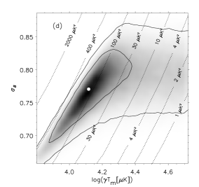
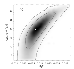
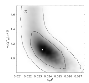
Figure 3: Top: mean 1D likelihoods for the Jeans length $\gamma T_{m}$, $\sigma_{8}$ and the rms temperature anisotropy contribution of the kSZ component. Each line correspond to a different fraction of baryons in the form of WHIM. In (b) we also plot the likelihood for the concordance (no kSZ) model. Bottom: mean 2D likelihoods for three different combinations of parameters. Solid lines depict the 1$\sigma$ and 2$\sigma$ confidence regions, and the thick dots indicate the positions of the likelihood maxima found in the full parameter space. Dotted curves in (d) represent levels with the same kSZ amplitude.

In Figures 3a,b,c we plot the mean 1D likelihoods for $\gamma T_{m}$, $\sigma_{8}$ and the more informative rms temperature fluctuation introduced by the kSZ signal defined as:

$$<\Delta{\rm T_{kSZ}}^{2}>^{1/2}=\left[\frac{1}{4\pi}\sum_{\ell=2}^{1000}(2\ell+1)C_{\ell}^{\rm kSZ}\right]^{1/2}~{}~{}.$$ (9)

The different lines correspond to different baryon fractions. Since the kSZ parameters affect the amplitude of the spectrum most significantly (see Figure 2) then, for each $f_{\rm b}$ the maximum 1D likelihood of $\gamma T_{m}$ shifts but the kSZ signal remains roughly constant (see Figure 3c). This high degeneracy indicates that 5 year WMAP data is insensitive to the fraction of baryons in the WHIM and hereafter we will quote results for $f_{\rm b}=0.5$.

In Figures 3d,e,f we show the mean 2D likelihoods for pairs of parameters. Solid lines represent 1$\sigma$ and 2$\sigma$ contours, whereas the white dots indicate the positions of the maximum likelihood in the full parameter space. Not unexpectedly, their positions are slightly shifted with respect to the 2D likelihood maxima. In fact, Markov chains estimate confidence intervals more precisely than locate the maximum of the likelihood, the bias being larger the greater the model dimensionality (Liddle, 2004). Figure 3d shows a noticeable degeneracy between $\sigma_{8}$ and ${\rm log}(\gamma T_{m})$. Within the 1$\sigma$ confidence region $A_{\rm kSZ}$ varies between $\sim 20~{}\mu$K² and $\sim 300~{}\mu$K². Regions with high values of $\sigma_{8}$ and low values of ${\rm log}(\gamma T_{m})$ are strongly ruled out since they overpredict the kSZ contribution. At the 2$\sigma$ level absence of a kSZ contribution is compatible with the data. This is also seen in Figures 3d,e. Models with kSZ prefer a lower value of $\sigma_{8}$ (see Figure 3b), since adding kSZ requires less primordial CMB power. Figure 3e(f) shows that $\Omega_{\rm b}h^{2}$ is (inversely) proportional to $\langle T_{\rm kSZ}^{2}\rangle^{1/2}$ (log[$\gamma T_{m}$]). Physically, kSZ adds power mainly at $\ell\sim$ 400–600 and the amplitude of the second acoustic peak gets reduced to fit the data. As a result, the best-fit value for $\Omega_{\rm b}h^{2}$ increases.

The parameters that maximize the likelihood are given in Table 2. The $1\sigma$ confidence intervals have been computed from the 1D mean likelihood distributions. The values for the concordance model agree well with those given by the WMAP team (Dunkley et al., 2009), indicating that we are correctly exploring the parameter space. The model with kSZ has larger error bars, as we are fitting the same data with an extra degree of freedom. The best-fit model has a kSZ power spectrum with a maximum amplitude of $A_{\rm kSZ}=129^{+138}_{-52}~{}\mu$K² centred at $\ell\approx 438$, corresponding to $\gamma T_{m}=1.3^{+0.4}_{-0.2}\times 10^{4}$ K. The rms temperature fluctuation is $\langle T_{\rm kSZ}^{2}\rangle^{1/2}=19^{+7}_{-9}~{}\mu$K, very significant compared with the contribution from the primordial CMB, $\langle T_{\rm CMB}^{2}\rangle^{1/2}=110~{}\mu$K. None of the parameters except $\Omega_{\rm b}h^{2}$ differ by more than 1$\sigma$ from those of the concordance model. The model with kSZ gives a higher value for $\Omega_{\rm b}h^{2}$. This reinforces the slight discrepancy between the values obtained from CMB temperature anisotropies and from BBN. As indicated above, adding kSZ boosts the value of $\Omega_{\rm b}h^{2}$ since it reduces the height of the second acoustic peak. The difference in $\sigma_{8}$ is also notable even if the confidence regions overlap at the 1$\sigma$ level. Our estimate is closer to the values obtained from the number density of galaxy clusters and the optical or X-ray cluster mass functions. For example, Voevodkin & Vikhlinin (2004) found $\sigma_{8}=0.72\pm 0.04$ from the baryon mass fraction of a sample of 63 X-ray clusters. After compiling cluster determinations since 2001 Hetterscheidt et al. (2007) obtained $\sigma_{8}=0.728\pm 0.035$, whereas from another compilation of the weak lens cosmic shear they found $\sigma_{8}=0.847\pm 0.029$.

In Figure 4a we compare the accuracy of the fitting of the two models to the 5 year WMAP data. We plot the best-fit power spectra for the models with and without kSZ after subtracting the WMAP band powers. The kSZ model achieves a better fit to the experimental data points in the multipole range $\ell\sim$ 300-700. The same conclusion can be obtained from Figure 4b, where we plot the ratio of the binned $\chi^{2}$ per $\ell$-band for the model without and with kSZ (note that these values were calculated, just for illustrative purposes, by applying the $\chi^{2}$ statistics to the binned best-fit theoretical power spectra, and not by the WMAP likelihood code). This ratio is overall $>1$ in the range $\ell\sim$ 300-700, even though within this interval there are some particular bins where the concordance model produces a slightly better fit.

Introducing the kSZ component, the $\chi^{2}$ reduces by $\Delta\chi^{2}=-3.3$, from 2661.05 to 2657.83. Evaluating the statistical significance of this result requires taking into account the number of degrees of freedom, given by the difference between the number of independent data points $N$ and of model parameters $k$. The WMAP likelihood is computed as a sum of different temperature and polarization terms (Dunkley et al., 2009). In this computation 968 points correspond to the TT power spectrum at $\ell=33$–1000 and 427 to the TE cross-correlation at $\ell=24$–450. For low ($\ell\leq 23$) multipoles the likelihood associated with the TT, TE, EE and EB correlations is evaluated directly from 1170 pixels of the temperature and polarization maps. In total $N=2565$. Adding the kSZ contribution raises the number of parameters from $k=6$ to $k=7$. Note that the $\chi^{2}$ per degree of freedom also decreases when the kSZ component is included, from $\chi^{2}_{\rm dof}=1.0399$ to 1.0390. Increasing the number of model parameters always improves the fit to a particular dataset but the model loses predictive power. In Bayesian statistics, information criteria can be used to decide whether the introduction of a new parameter is favored by the data. Examples are the Akaike information criterion (Akaike, 1974) defined as AIC $=2k+\chi^{2}$ or the more conservative Bayesian information criterion (Schwarz, 1978) BIC $=\chi^{2}+k{\rm ln}N$. Since we are adding a single parameter, we obtain $\Delta$AIC $=-1.2$, which is marginal evidence in favor of introducing this new parameter while $\Delta$BIC $=4.1$ is evidence against it, reflecting the fact that no kSZ component is compatible with the data at the 2$\sigma$ level. Even if at present model selection does not clearly favors the kSZ contribution, it is a model well motivated physically and, as remarked by Linder & Miquel (2008), model selection needs to involve physical insight. A statistically more significant measurement would require a wider frequency coverage and angular resolution, as will be provided by the forthcoming Planck mission.

The kSZ contribution represents 3.1% of the power measured in 5 year WMAP data. This contribution is larger than expected; typical filaments would give rise to $\Delta T_{\rm kSZ}\sim$ 2–5 $\mu$K (eq. 7). We would need a more accurate (numerical) model to establish which would be the physical conditions that give rise to the quoted kSZ signal. Numerical simulations over large cosmological volumes are computationally very expensive because they require high resolution over most of the volume. In fact, spatial resolution is usually an important limitation. Adaptive mesh refinement (AMR) techniques are efficient at describing the dynamics of gas in the high dense regions but their resolution falls sharply in less dense environments (Refregier & Teyssier, 2002), while smooth particle hydrodynamics (SPH) codes do not yet resolve scales as small as the Jeans length (Bond et al., 2005), that effectively dominate the WHIM SZ contribution (Atrio-Barandela & Mücket, 2006). Hallman et al. (2007) used the AMR Enzo code (O’Shea et al., 2005) to simulate a (512 Mpc/h)³ volume including unbound bas, and found that one-third of the SZ flux in a 100 square-degree region comes from objects with masses below $5.0\times 10^{13}$ M_⊙ and filamentary structures made up of WHIM gas, a conclusion similar to that reached by Hernández-Monteagudo et al. (2006). Hallman et al. (2009) focused in the low-density WHIM gas by restricting their analysis of the same AMR simulation to regions with temperatures in the range $10^{5}-10^{7}$ K and overdensities $\delta<50$, even though their low mass halos were not yet resolved gravitationally. They computed the radiation power spectrum from that simulation and found a similar shape to that of Figure 1, although with a much smaller amplitude. The high amplitude we found could be an indirect confirmation of large scale peculiar motions reported in Kashlinsky et al. (2008) and Kashlinsky et al. (2009). If bulk flows of this amplitude are very common, filaments at higher redshift could also contribute significantly, thereby increasing the total signal. Also, we must take into account a possible foreground contamination: power spectra with a single maximum are also good models for Poissonianly distributed foreground residuals or unresolved point sources. Since the WMAP window function exponentially damps power at $\ell\gtrsim 600$, the convolution of a $C_{\ell}$ = const. spectrum with this window function peaks at $\ell<600$ and has a shape similar to that of the spectrum described above. Foreground substraction can differ in the range 3–5 $\mu$K depending on the method (Ghosh et al., 2009) and some residuals could be present on the data at that level. To distinguish the WHIM kSZ and foreground signals we will have to include the frequency dependence, amplitude and location of the maximum for each component. In the simplest model with kSZ and one foreground, we would need four parameters to model both components so an analysis of all components is unfeasible with WMAP 3 frequency bands (Q, V and W).

To conclude, we have explored the parameter space of the concordance model to show that the WHIM kSZ contribution could be as high as 3% the total power of 5 year WMAP data. This large amplitude is difficult to account for in the concordance $\Lambda$CDM model, where filaments are expected to have $\lesssim 5~{}\mu$K contributions. It could be an indication that large scale flows are rather common. We cannot rule out that part of this contribution could be due to unmasked point sources and/or foreground residuals. The Planck satellite, with its wider frequency coverage, lower noise and different scanning strategy, is well suited for detecting the IGM/WHIM thermal and kinematic contributions with much higher statistical significance and to distinguishing this signal from other foreground contributions.

We are thankful to Rafael Rebolo for enlightening discussion and suggestions. This work is supported by the Ministerio de Educación y Ciencia and the “Junta de Castilla y León” in Spain (FIS2006-05319, programa de financiación de la actividad investigadora del grupo de Excelencia GR-234).

Figure 1: (a) Intrinsic CMB radiation power spectrum (solid line) and the IGM/WHIM tSZ and kSZ (dashed lines) contributions. (b) Contributions of redshift intervals to the total tSZ spectrum. From left to right, solid lines correspond to contributions from the following redshift intervals: [0,0.005], [0.005,0.05], [0.05,0.1], [0.1,0.2], [0.2,0.3] and [0.3,0.4]. (c) Redshift contribution to the kSZ effect. Solid lines give the contribution for $z=0$ to $0.1$ with spacing $\Delta z=0.01$; dotted lines give the contributions for $z=0.1$ to $0.4$ with $\Delta z=0.1$. Dashed lines show the total power spectra from all the redshift intervals. The SZ contributions are calculated in all cases using $\sigma_{8}=0.77$, $\gamma=1.3$, $\gamma T_{m}=1.3\times 10^{4}$ K and $f_{\rm b}=0.5$.

Figure 2: Kinematic Sunyaev–Zel’dovich power spectra from WHIM for a fixed $\sigma_{8}=0.80$ and different values of $\gamma T_{m}$ (solid lines), and for a fixed $\gamma T_{m}=1.3\times 10^{4}$ K and different values of $\sigma_{8}$ (dotted lines). The fraction of baryons stored in the form of WHIM has been fixed at $f_{\rm b}=0.5$ in all cases.

Basic	Parameter	Starting	Distribution
parameter	limits	points	width
$\Omega_{\rm b}h^{2}$	(0.005, 0.1)	0.0223	0.001
$\Omega_{\rm cdm}h^{2}$	(0.01, 0.99)	0.105	0.01
100$\theta$	(0.5, 10)	1.04	0.002
${\rm ln}(10^{10}A_{\rm S})$	(2.7, 4.0)	3.0	0.01
$n_{\rm s}$	(0.5, 1.5)	0.95	0.01
$\tau$	(0.01, 0.8)	0.09	0.03
${\rm log}(\gamma T_{m})$	(3.778, 4.740)	4.096	0.006

Table 1: For each independent parameter, we indicate its range of variation (top-hat prior), the initital values and the estimated distribution widths initially used by the chain to vary each parameter.

Parameter	CMB alone	CMB and kSZ
$\Omega_{\rm b}h^{2}$	$0.0223^{+0.0007}_{-0.0006}$	$0.0234^{+0.0020}_{-0.0008}$
$\Omega_{\rm cdm}h^{2}$	$0.1086^{+0.0081}_{-0.0060}$	$0.1096^{+0.0068}_{-0.0085}$
100$\theta$	$1.040^{+0.004}_{-0.003}$	$1.042^{+0.005}_{-0.004}$
${\rm ln}(10^{10}A_{\rm S})$	$3.06\pm 0.05$	$3.02^{+0.05}_{-0.08}$
$n_{\rm s}$	$0.96\pm 0.02$	$0.95\pm 0.02$
$\tau$	$0.088^{+0.020}_{-0.019}$	$0.087^{+0.023}_{-0.017}$
$\gamma T_{\rm m}$ (104K)		$1.31^{+0.41}_{-0.23}$
$\Omega_{\Lambda}$	$0.745^{+0.027}_{-0.042}$	$0.752^{+0.043}_{-0.034}$
$\Omega_{\rm m}$	$0.255^{+0.042}_{-0.027}$	$0.248^{+0.034}_{-0.043}$
$\sigma_{8}$	$0.793^{+0.042}_{-0.037}$	$0.771^{+0.039}_{-0.069}$
$z_{\rm re}$	$10.57^{+1.37}_{-1.73}$	$10.14^{+1.51}_{-1.57}$
$H_{0}$	$71.63^{+2.85}_{-3.12}$	$73.18^{+6.15}_{-2.60}$
$\langle T_{\rm kSZ}^{2}\rangle^{1/2}$ ($\mu$K)		$19.5^{+6.8}_{-8.7}$
$A_{\rm kSZ}$ ($\mu$K2)		$128.7^{+138.0}_{-52.3}$
$\chi^{2}$	2661.05	2657.83

Table 2: Best-fit parameters for the model without and with a kSZ contribution. These results correspond to a fraction of baryons in the form of WHIM of $f_{\rm b}=0.5$. The upper and lower (below the line) sets correspond to independent and derived parameters, respectively. The central values have been derived from the sample with the minimum $\chi^{2}$ in the chains (also shown in the table), whereas the 1$\sigma$ confidence limits were derived from the 0.159 and 0.841 points of the cumulative probability distribution given by the 1D mean likelihoods.

Figure 4: Top: best-fit power spectra for the models with (solid line) and without (dotted line) kSZ, after subtracting the WMAP experimental band powers. The vertical lines represent the 1$\sigma$ error bars of the 5 year WMAP data. Bottom: ratio of the $\chi^{2}$ in $\ell$-bands of width $\Delta\ell=15$ for a model without and with a kSZ component.

References

- Akaike (1974) Akaike, H. 1974, IEEE Trans. Aut. Cont. 19(6), 716