Reverberation Mapping of the Optical Continua of 57 MACHO Quasars

1 Abstract

Autocorrelation analyses of the optical continua of 57 of the 59 MACHO quasars reveal structure at proper time lags of $544\pm 5.2$ days with a standard deviation of 77 light days. Interpreted in the context of reverberation from elliptical outflow winds as proposed by Elvis (2000) [1], this implies an approximate characteristic size scale for winds in the MACHO quasars of $544\pm 5.2$ light days. The internal structure variable of these reflecting outflow surfaces is found to be $11.87^{o}\pm 0.40^{o}$ with a standard deviation of $2.03^{o}$.

2 Introduction

Brightness fluctuations of the UV-optical continuum emission of quasars were recognised shortly after the initial discovery of the objects in the 1960s [2]. Although several programmes were undertaken to monitor these fluctuations, little is yet known about their nature or origin. A large number of these have focused on comparison of the optical variability with that in other wavebands and less on long-timescale, high temporal resolution optical monitoring. Many studies have searched for oscillations on the $\sim$ day timescale in an attempt to constrain the inner structure size (eg [3]). This report, however, is concerned with variability on the year timescale to evidence global quasar structure.

In a model proposed by Elvis [1] to unite the various spectroscopic features associated with different “types” of quasars and AGN (eg broad absorption lines, X-ray/UV warm absorbers, broad blue-shifted emission lines), the object’s outer accretion disc has a pair of bi-conical extended narrow emission line regions in the form of outflowing ionised winds. Absorption and emission lines and the so-called warm absorbers result from orientation effects in observing these outflowing winds. Supporting evidence for this is provided by a correlation between polarisation and broad absorption lines found by [4]. Outflowing accretion disc winds are widely considered to be a strong candidate for the cause of feedback (for a discussion of the currently understood properties of feedback see [5]). Several models have been developed [6, 7] to simulate these winds. [6] discusses different launch mechanisms for the winds - specifically the balance between magnetic forces and radiation pressure - but finds no preference for one or the other, while [7] discusses the effect of rotation and finds that a rotating wind has a larger thermal energy flux and lower mass flux, making a strong case for these winds as the source of feedback. The outflow described by [1] is now usually identified with the observationally-invoked “dusty torus” around AGN [8].

[9] demonstrated for the MACHO quasars that there is no detectable lag time between the V and R variability in quasars, which can be interpreted as demonstrating that all of the optical continuum variability originates in the same region of the quasar.

[10] observed the gravitationally lensed quasar Q0957+561 to measure the time delay between the two images and measure microlensing effects. In doing so, they found a series of autocorrelation subpeaks initially attributed to either microlensing or accretion disc structure. These results were then re-interpreted by [11] as Elvis’ outflowing winds at a distance of $2\times 10^{17}cm$ from the quasar’s central compact object. A model applied by [12] to the quasar Q2237+0305, to simulate microlensing, found that the optimal solution for the system was one with a central bright source and an extended structure with double the total luminosity of the central source, though the outer structure has a lower surface brightness as the luminosity is emanating from a larger source, later determined by [13] to lie at $8.4\times 10^{17}cm$.

[13] continued on to argue that since magnetic fields can cause both jets and outflows, they therefore must be the dominant effect in AGN. [14] however pointed out that the magnetic field required to power the observed Elvis outflows is too great to be due to the accretion disc alone. They therefore argue that all quasars and AGN have an intrinsically magnetic central compact object, which they refer to as a MECO, as proposed by [15], based upon solutions of the Einstein-Maxwell equations by [16]. One compelling aspect to this argument is that it predicts a power-law relationship between Elvis outflow radius and luminosity, which was found in work by Kaspi et al [17] and updated by Bentz et al [18], if one assumes the source of quasar broad emission lines to be outflow winds powered by magnetic fields. The [17] and [18] results were in fact empirically derived for AGN of $Z<0.3$ and [17] postulates that there may be some evolution of this relation with luminosity (and indeed one might expect some time-evolution of quasar properties which may further modify this scaling relation) so generalising these results to quasars may yet prove a fallacy. The radius of the broad line region was found to scale initially by [17] as $R_{blr}\propto L^{0.67}$, while [18] found $R_{blr}\propto L^{0.52}$.

Another strength of the MECO argument is that while [19] found quasar properties to be uncorrelated using the current standard black hole models, [14] and [20] found a homogeneous population of quasars using the [16] model. [21] used microlensing observations of 10 quadruply-lensed quasars, 9 of which were of known redshift including Q2237+0305, to demonstrate that standard thin accretion disc models, such as the widely-accepted Shakura-Sunyaev (S-S) disc [22], underestimate the optical continuum emission region thickness by a factor of between 3 and 30, finding an average calculated thickness of $3.6\times 10^{15}cm$, while observed values average $5.3\times 10^{16}cm$. [23] found a radius of the broad line region for the Seyfert galaxy NGC 5548 of just under 13 light days when the average of several spectral line reverberations were taken, corresponding to $R_{blr}=3.3\times 10^{16}cm$. When the scaling of [17] and [18] is taken into account, the [23] result is comparable to the [13] and [11] results (assuming $\frac{L_{quasar}}{L_{seyfert}}\sim 10^{4}$, then [18] would predict a quasar $R_{blr}$ of approximately $3\times 10^{18}$). Also, given that black hole radius scales linearly with mass, as does the predicted radius of the inner edge of the accretion disc, a linear mass-$R_{blr}$ relationship might also be expected. Given calculated Seyfert galaxy black hole masses of order $10^{8}M_{o}$ and average quasar masses of order $10^{9}M_{o}$, this would scale the Seyfert galaxy $R_{blr}$ up to $3.3\times 10^{17}cm$. While these relations are not self-consistent, either of them may be found consistent with the existing quasar structure sizes. [24] also found structure on size scales of $10^{16}cm$ from microlensing of SDSS J1004+4112 which would then scale to $10^{18}cm$. These studies combined strongly evidence the presence of the Elvis outflow at a radial distance of approximately $10^{18}cm$ from the central source in quasars which may be detected by their reverberation of the optical continuum of the central quasar source.

The [12] result is also in direct conflict with the S-S accretion disc model, which has been applied in several unsuccessful attempts to describe microlensing observations of Q2237. First a simulation by [25] used the S-S disc to model the microlensing observations but predicted a large microlensing event that was later observed not to have occurred. [26] then attempted to apply the S-S disc in a new simulation but another failed prediction of large-amplitude microlensing resulted. Another attempt to simulate the Q2237 light curve by [27] produced the same large-amplitude microlensing events. These events are an inherent property of the S-S disc model where all of the luminosity emanates from the accretion disc, hence causing it all to be lensed simultaneously. Only by separating the luminosity into multiple regions, eg two regions, one inner and one outer, as in [12], can these erroneous large-amplitude microlensing events be avoided.

Previous attempts have been made to identify structure on the year timescale, including structure function analysis by Trevese et al [28] and by Hawkins [29, 30]. [28] found strong anticorrelation on the $\sim 5$ year timescale but no finer structure - this is unsurprising as their results were an average of the results for multiple quasars taken at low temporal resolution, whereas the size scales of the Elvis outflow winds should be dependant on various quasar properties which differ depending on the launch mechanism and also should be noticed on smaller timescales than their observations were sensitive to. [29] also found variations on the $\sim 5$-year timescale again with poor temporal resolution but then put forth the argument that the variation was found to be redshift-independant and therefore was most likely caused by gravitational microlensing. However [31] demonstrated that microlensing occurs on much shorter timescales and at much lower luminosity amplitudes than these long-term variations. [30] used structure function analysis to infer size scales for quasar accretion discs but again encountered the problem of too infrequent observations. In this paper and [32] it was argued that Fourier power specra are of more use in the study of quasars, which were then used in [32] to interpret quasar variability. However, since reverberation is not expected to be periodic, Fourier techniques are not suited to its detection. Hawkins’ observations of long-timescale variability were recognised in [33] as a separate phenomenon to the reverberation expected from the Elvis model; this long-term variability remains as-yet unexplained. Hawkins’ work proposed this variation to be indicative of a timescale for accretion disc phenomena, while others explained it simply as red noise.

[34] demonstrated that there is a correlation between the optical and x-ray variability in some but not all AGN, arguing that x-ray reprocessing in the accretion disc is a viable source of the observed variability, combined with viscous processes in the disc which would cause an inherent mass-timescale dependance, as in the S-S disc the temperature at a given radius is proportional to mass${}^{-\frac{1}{4}}$. In this case a red-noise power spectrum would describe all quasar variability. For the purposes of this report however, the S-S disc model is regarded as being disproven by the [12] and [21] results in favour of the Elvis outflow model and so the temperature-mass relation is disregarded. A later investigation [35] demonstrated that the correlation between X-ray and optical variability cannot be explained by simple reprocessing in an optically thick disc model with a corona around the central object. This lends further support to the assumption that the [12] model of quasars is indeed viable.

[36] demonstrated from Fourier power spectra that shorter-duration brightness events in quasars statistically have lower amplitudes but again their temporal resolution was too low to identify reverberation on the expected timescales. Also as previously discussed, non-periodic events are extremely difficult to detect with Fourier techniques. All of these works are biased by the long-term variability recognised by [33] as problematic in QSO variability study. A survey by [37] proposed that quasars could be identified by their variability on this timescale but the discovery by [33] that long-timescale variation is not quite a universal property of quasars somewhat complicates this possibility. The spread of variability amplitudes is also demonstrated in [38] for 44 quasars observed at the Wise Observatory. The [38] observations are also of low temporal resolution and uncorrected for long-term variability thus preventing the detection of reverberation patterns.

This project therefore adopts the [1] and [12] model of quasars consisting of a central compact, luminous source with an accretion disc and outflowing winds of ionised material with double the intrinsic luminosity of the central source. The aim is to search for said winds via reverberation mapping. Past investigations such as [39] have attempted reverberation mapping of quasars but have had large gaps in their data, primarily due to the fact that telescope time is usually allocated only for a few days at a time but also due to seasonal dropouts. Observations on long timescales, lacking seasonal dropouts and with frequent observations are required for this purpose, to which end the MACHO programme data have been selected. Past results would predict an average radius of the wind region of order $10^{18}cm$.

The assumption will be made that all structure on timescales in the region of $c\Delta t=10^{18}cm$ is due to reverberation and that the reverberation process is instantaneous. The aim is simply to verify whether this simplified version of the model is consistent with observation, not to compare the model to other models.

3 Theoretical Background

Reverberation mapping is a technique whereby structure size scales are inferred in an astrophysical object by measuring delay times from strong brightness peaks to subsequent, lower-amplitude peaks. The subsequent peaks are then assumed to be reflections (or absorptions and re-emissions) of the initial brightness feature by some external structure (eg the dusty torus in AGN, accretion flows in compact objects). Reverberation mapping may be used to study simple continuum reflection or sources of specific absorption/emission features or even sources in entirely different wavebands, by finding the lag time between a brightness peak in the continuum and a subpeak in the emission line or waveband of interest. This technique has already been successfully applied by, among many others, [23] and [11].

When looking for continuum reverberation one usually makes use of the autocorrelation function, which gives the mean amplitude, in a given light curve, at a time $t+\Delta t$ relative to the amplitude at time $t$. The amplitude of the autocorrelation is the product of the probability of a later brightening event at dt with the relative amplitude of that event, rendering it impossible to distinguish by autocorrelation alone, eg a 50% probability of a 50% brightening from a 100% probability of a 25% brightening, since both will produce the same mean brightness profile. The mathematical formulation of this function is:

$$AC(\Delta t)=\frac{1}{N_{obs}}\cdot\sum_{t}\frac{I(t+\Delta t)\cdot I(t)}{\sigma^{2}}$$ (1)

where I(t) represents the intensity at a time t relative to the mean intensity, such that for a dimming event I(t) is negative. Hence $AC(\Delta t)$ becomes negative if a brightening event at t is followed by a dimming event at $t+\Delta t$ or if a dimming event at t is followed by a brightening event at $t+\Delta t$. $\sigma$ is the standard deviation of I - in rigorous mathematics the $\sigma^{2}$ term is in fact the product of the standard deviations for I(t) and I($t+\Delta t$) but since they are idential in this case, $\sigma^{2}$ may be used. The nature of the autocorrelation calculation also has a tendancy to introduce predicted brightness peaks unrelated to the phenomena of interest. Given autocorrelation peaks at lag times $t_{1}$ and $t_{2}$, a third peak will also be created at lag $t_{2}-t_{1}$, of amplitude $\frac{A(t_{2})}{A(t_{1})}$, which is then divided by the number of data points in the brightness record.

4 Observational Details

The MACHO survey operated from 1992 to 1999, observing the Magellanic Clouds for gravitational lensing events by Massive Compact Halo Objects - compact objects in the galactic halo, one of the primary dark matter candidates. The programme was undertaken from the Mount Stromlo Observatory in Australia, where the Magellanic Clouds are circumpolar, giving brightness records free from seasonal dropouts. Information on the equipment used in the programme can be found at http://wwwmacho.anu.edu.au/ or in [40]. 59 quasars were within the field of view of this programme and as a result highly sampled light curves for all of these objects were obtained. These quasars were observed over the duration of the programme in both V and R filters. The brightness records for the 59 quasars in both V and R filters are freely available at http://www.astro.yale.edu/mgeha/MACHO/ while the entire MACHO survey data are available from http://wwwmacho.anu.edu.au/Data/MachoData.html.

5 Theoretical Method

Throughout this study the following assumptions were made:

1. That all autocorrelation structure on the several hundred day timescale was due to reverberation from the Elvis outflows, which are also the source of the broad emission lines in quasars. We denote the distance to this region as $R_{blr}$ - the “radius of the broad line region”.

2. That the timescale for absorption and re-emission of photons was negligable compared to the light travel time from the central source to the outflow surface.

3. That the internal structure variable was less than $45^{o}$ for all objects as found by [11] and [13]. Note that an internal structure variable of $\epsilon$ and inclination angle of $\theta$ cannot be distinguished by autocorrelation alone from an internal structure variable of $90^{o}-\epsilon$ with an inclination angle of $90^{o}-\theta$, as demonstrated in Fig. 1. The assumed low $\epsilon$ is further justified by the fact that the [1] model predicts the winds to be projected at an angle of $30^{o}$ from the accretion disc plane, contraining $\epsilon\leq 30^{o}$ as the reverberating surfaces must lie at lower inclinations if they are in fact part of the outflow structure.

4. That extinction was negligable for all objects. Reliable extinction maps of the Magellanic Clouds are not available and information about the quasars’ host galaxies is also unavailable so extinction calculations are not possible. This assumption should be reasonable as any extinction would have a noticeable impact on the colour of the quasar (given the accepted relation $3.2\cdot E(B-V)=A_{V}$ where $E(B-V)$ is the colour excess and $A_{V}$ is the V absorption).

First a series of predictions were made for the relative luminosities of the 59 quasars in the sample using their redshifts (presented in [41]) and apparent magnitudes, combined with the mean quasar SED presented in [42]. Two estimates were produced for these, one for the V data and one for the R data. This calculation was of interest as it would predict the expected ratios of $R_{blr}$ between the objects in our sample via the [17] and [18] relations. These relations are so far only applied to nearby AGN and so this investigation was carried out to test their universality. Firstly, the apparent magnitudes were converted to flux units via the equation

$$m=-2.5\cdot\log{f}$$ (2)

where m is the apparent magnitude and f the flux. Then the redshifts of the objects were used to calculate their distances using the tool at
http://astronomy.swin.edu.au/ elenc/Calculators/redshift.php with $H_{0}=71Mpc/km/s$. Using this distance and the relation

$$f=\frac{L}{4\pi d^{2}}$$ (3)

where L is the luminosity, f the flux and d the distance, the luminosity of each source in the observed waveband was calculated. It was recognised, however, that simply taking the ratio between these luminosities was not a fair representation of the ratio of their absolute luminosities as cosmological redshift would cause the observed region of the quasar spectrum to shift with distance and the luminosity varies over the range of this spectrum. Hence the mean quasar SED of [42] was used to convert the observed luminosities of the objects to expected luminosities at a common frequency - in this case 50 GHz. These values were then divided by the minimum calculated luminosity so that their relative values are presented in Table 1. For this purpose it was assumed that the spectral shape of the quasar is independant of bolometric luminosity.

Next a calculation was made to predict the dependance of the reverberation pattern of a quasar on its orientation to the observer’s line of sight. This was produced using the geometric equations initially presented in [11] but reformulated to become more general. [11] discusses ”case 1” and ”case 2” quasars with different orientations - ”case 1” being where the nearest two outflow surfaces lie on the near side of the accretion disc plane and ”case 2” being where the nearest two surfaces are on the near side of the rotation axis. These equations become generalised by recognising that the two cases are in fact degenerate and from reverberation alone one cannot distinguish a $13^{o}$ internal structure variable in ”case 1” from a $77^{o}$ internal structure variable in ”case 2”. This is also demonstrated in Fig. 1. For the purposes of Fig. 1, the [11] interpretation of $\epsilon$ is adopted but later it will be demonstrated that in fact there are several possible meanings of $\epsilon$, though this degeneracy is the same for all interpretations.

(a) $\epsilon$ and $\theta$ as in Case I of [11]

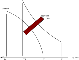
(b) $\theta^{1}=\epsilon$ and $\epsilon^{1}=\theta$

(c) $\theta^{1}=90^{o}-\theta$ and $\epsilon^{1}=90^{o}-\epsilon$

Figure 1: Three different quasar orientations and internal structure variables can give the same series of reverberation lags

The generalisation is then

$$t_{1}=\frac{R_{blr}}{c}\cdot(1-\cos(\theta-\epsilon))$$ (4)

$$t_{2}=\frac{R_{blr}}{c}\cdot(1-\cos(\theta+\epsilon))$$ (5)

$$t_{3}=\frac{R_{blr}}{c}\cdot(1+\cos(\theta+\epsilon))$$ (6)

$$t_{4}=\frac{R_{blr}}{c}\cdot(1+\cos(\theta-\epsilon))$$ (7)

This prediction could later be compared to the MACHO observations. A value of $\epsilon$ was not inserted until the project had produced results, so that the mean calculated value of $\epsilon$ could be inserted into the simulation for comparison with the results.

In the data analysis it was quickly noticed that one of the 59 MACHO quasars - MACHO 42.860.123 - was very poorly observed by the survey, totalling only 50 observations over the programme’s seven-year lifetime. The V and R data for the remaining objects were processed in IDL to remove any 10-$\sigma$ data points – 5-$\sigma$ would seem a more appropriate value at first glance, but inspection of the data showed relevant brightness peaks between 5- and 10-$\sigma$. At the same time all null entries (nights with no observation) were also removed. The data were then interpolated to give a uniformly-spaced brightness record over time, with the number of bins to interpolate over equal to the number of observations. The case was made for using a fixed number of bins for all objects, eg 1000, but for some data records as few as 250 observations were made and so such an interpolation would serve only to reinforce any remaining spurious points. By the employed method, a small amount of smoothing of the data was introduced. The data then had their timescales corrected for cosmological redshift to ensure that all plots produced and any structure inferred were on proper timescales.

In the beginning of the project, to understand the behaviour of the data and appreciate the complexities and difficulties of the investigation, a list was compiled of the most highly-sampled ($>600$ observations) quasars, yielding 30 objects. Each of these objects had their light curves and autocorrelations examined and a key feature presented itself immediately; the data showed in some cases a long-timescale ($\sim 1000$ proper days), large-amplitude ($\sim 0.8$ magnitude) variation that dominated the initial autocorrelation function. Since this variation was seen only in some quasars (and is on a longer timescale than the predicted reverberation), this signal was removed by applying a 300-day running boxcar smooth algorithm over the data, before subtracting this smoothed data (which would now be low-frequency variation dominated) from the actual brightness record. The timescale for smoothing was determined by examination of the brightness profiles of the objects, which showed deviations from this long-timescale signature on timescales below 300 days. Autocorrelation analysis of the uncorrected data also found the first autocorrelation minimum to lie before 300 days. Further, if the central brightness pulse has a duration beyond 300 days it will be extremely difficult (if even possible) to resolve the delay to the first reverberation peak, which is expected to be at a maximum lag time of several hundred days. The new autocorrelation calculations for the long-term variability-corrected data showed from visual inspection the autocorrelation patterns expected from reverberation. However, as is described in section 2, the presence of autocorrelation peaks alone do not necessarily constitute a detection of reverberation.

To determine the reality of the autocorrelation peaks, a routine was written to identify the ten largest-amplitude brightening and fading events in each low-pass filtered brightness record and produce the mean brightness profiles following them - a mean brightening profile and a mean dimming profile. Inspection of these brightness profiles demonstrated that any spurious autocorrelation peaks were a small effect, easily removed by ignoring any peaks within one hundred days of a larger-amplitude peak. The justification for this is simple - if two reverberations occur within one hundred days of each other (which has a low probability of occurence when one considers the required quasar orientation), resolving them within the brightness record or autocorrelation will become difficult, particularly for the most poorly-sampled, low-redshift objects with a time resolution of $\sim 10$ days and given that the average half-width of a central brightness peak was found to be approximately 70 days. There is also the consideration of the shape of the reverberation signal from each elliptical surface, which has not yet been calculated but may have differing asymmetry for each of the four surfaces.

Finally it was noticed that the brightening and dimming profiles do not perfectly match and in some cases seem to show structure of opposing sign on the same timescales - if a brightening event was usually followed by another brightening event at a time lag $t$, a dimming event was sometimes also followed by a brightening event at a lag of $t$. The fact that this effect is not seen in every object makes it difficult to interpret or even identify as a real effect. The result of this is that the mean brightness profile does not always perfectly match the autocorrelation, but usually demonstrates the same approximate shape. These arguments are not quantifiable and so are discarded from future investigation, which will focus on the results of an automated analysis. At this point it was also noted that the highest-redshift quasar in the survey, MACHO 208.15799.1085 at a redshift of 2.77, contained only $\sim 700$ proper days’ worth of observations. It was felt that this would not be sufficient time to observe a significant number of reverberation events, which were observed to occur on timescales of order $\sim 500$ proper days, and so the object was discarded from further analysis. Fig. 2 gives one example of the manually-produced light curves, its autocorrelation and the effect of long-term variability.

Figure 2: Plots produced in manual inspection of the data for one quasar. Top left is the raw data, top right its autocorrelation. On the bottom left is the data remaining after subtraction of long-term variability and bottom right is the corrected data’s autocorrelation function.

In the automatically-processed, long-term variability-corrected data, reverberation patterns were recognised in the autocorrelation by an IDL routine designed to smooth the autocorrelation on a timescale of 50 days and identify all positive peaks with lags less than 1000 days. If two or more peaks were identified within 100 days of each other, the more prominent peak was returned. As a result, we estimate the accuracy of any reverberation signatures to be approximately 50 days. Therefore a 50-day smooth will reduce the number of peaks for the program to sort through while not detracting from the results, simultaneously removing any double-peaks caused by dips in autocorrelation caused by unrelated phenomena. The 50-day resolution simply reflects the fact that the occurence of two peaks within one hundred days can not be identified with two separate reverberations.

This technique was also applied to a ’Brownian noise’ or simple red noise simulation with a spectral slope of -2 for comparison. This was generated using a random number generator in the following way. First an array (referred to as R) of N random numbers was produced and the mean value subtracted from each number in said array. A new, blank array (S) of length N+1 was created, with values then appended as follows:

$$\mbox{if }R[i]>0\mbox{ then }S[i+1]=S[i]+1$$ (8)

$$\mbox{if }R[i]<0\mbox{ then }S[i+1]=S[i]-1$$ (9)

The seeds for the random number generator were taken as the raw data for each quasar in each filter, so that 114 different simulations were produced to aid in later comparison with results. [43] outline a method for producing more rigorous red noise simulations of different spectral slopes but to allow more time to focus on the observations and their interpretation, only this simplified calculation was performed.

Basic white noise simulations were also produced but produced none of the predicted autocorrelation structure and so were only followed through the early data processing stages. An example white noise autocorrelation is given in Fig. 3 with a quasar autocorrelation curve overplotted. Fig. 4 shows the light curve and autocorrelation function for a star observed by the MACHO programme compared to one of the quasars to demonstrate the difference in autocorrelation function and demonstrate that the observed structure is a feature of the quasars themselves and not induced by observational effects.

Figure 3: Quasar (+) and white noise (.) autocorrelation functions

Figure 4: Top: Quasar (+) and star data (.) demonstrating that the long-term variability observed in the quasars is not an observational effect. Bottom: Quasar (bold) and star autocorrelation functions after 300-day boxcar smooths have been applied, showing that the autocorrelation structure observed in quasars is intrinsic to the quasars themselves

6 Results

Once the data were processed and autocorrelation peaks identified, the positions of the peaks were then used to calculate the radial distance from central source to outflow region ($R_{blr}$), the inclination angle of the observer’s line of sight from the accretion disc plane ($\theta$) and a factor termed the ’internal structure variable’ which is the angle from the accretion disc plane to the reverberating outflow regions ($\epsilon$). These are calculated from equations (2-5). These can then produce

$$(4)+(5)+(6)+(7)=t_{1}+t_{2}+t_{3}+t_{4}=4\cdot\frac{R_{blr}}{c}$$ (10)

or $R_{blr}=c\cdot\langle t\rangle$

$$(6)-(5)=t_{3}-t_{2}=2\cdot\frac{R_{blr}}{c}\cdot\cos(\theta+\epsilon)$$ (11)

or $\theta+\epsilon=\arccos(\frac{t_{3}-t_{2}}{2\cdot\langle t\rangle})$

$$(7)-(4)=t_{4}-t_{1}=2\cdot\frac{R_{blr}}{c}\cdot\cos(\theta-\epsilon)$$ (12)

or $\theta-\epsilon=\arccos(\frac{t_{4}-t_{1}}{2\cdot\langle t\rangle})$

From (11) and (12) we then obtain

$$\theta=\frac{\arccos(\frac{t_{3}-t_{2}}{2\cdot\langle t\rangle})+\arccos(\frac{t_{4}-t_{1}}{2\cdot\langle t\rangle})}{2}$$ (13)

$$\epsilon=\frac{\arccos(\frac{t_{3}-t_{2}}{2\cdot\langle t\rangle})-\arccos(\frac{t_{4}-t_{1}}{2\cdot\langle t\rangle})}{2}$$ (14)

Consideration of the geometry involved also shows that three special cases must be considered. First is the case where $\theta=90^{o}-\epsilon$. In this case, peaks two and three are observed at the same time and so only three distinct brightness pulses are seen. In analysing the data, the simplifying assumption was made that all 3-peak autocorrelation signatures were caused by this effect. Another case to be considered is when $\theta=90^{o}$, in which cases pulses 1 and 2 are indistinguishable, as are pulses 3 and 4. Again, the assumption was made that all two-peak reverberation patterns were caused by this orientation effect. Notice that in these cases the equation for $R_{blr}$ is not modified, but the equations for $\epsilon$ in the 3-peak and 2-peak cases become

$$\epsilon=\frac{\arcsin(\frac{t_{3}-t_{1}}{2\cdot\langle t\rangle})}{2}$$ (15)

$$\epsilon=\frac{\arcsin(\frac{t_{2}-t_{1}}{2\cdot\langle t\rangle})}{2}$$ (16)

respectively. Finally there is the case of zero inclination angle, where peaks one and two arrive at the same time as the initial brightening event, followed by peaks three and four which then arrive simultaneously. In this situation no information about the internal structure variable can be extracted. Thankfully, no such events were observed. The results calculated for the 57 studied quasars, from equations (10) and (13-16), are presented in Table 1. The redshifts presented in Table 1 are as given in [41]. Additionally a column has been included showing $R_{blr}$ in multiples of the minimum measured $R_{blr}$ for comparison with the relative luminosities of the quasars.

This yields an average $R_{blr}$ of 544 light days with an RMS of 74 light days and an average $\epsilon$ of $11.87^{o}$ with an RMS of $2.03^{o}$. A plot of $t_{1}$, $t_{2}$, $t_{3}$, $t_{4}$ as a function of $\theta$ for the 57 objects was then compared to the predictions of a simulation using the calculated average $\epsilon$ from these observations, for the data from both filters. This entire process was then repeated for the red noise simulations, of which 114 were produced such that the resulting plots could be directly compared. The simulations produced by the R data were treated as R data while the simulations produced by V data were treated as V data, to ensure the simulations were treated as similarly to the actual data as possible. The process was then repeated for 10 stars in the same field as the example quasar that was studied in detail, MACHO 13.5962.237. Notice that while the quasar data show trends very close to the model, the star data exhibit much stronger deviations (see Fig. 5).

Table 1: Properties of the MACHO quasars. z is the quasar’s redshift, n(V) and n(R) the number of V and R band observations respectively, V and R respectively are the average V and R magnitudes, $R_{blr}$ the calculated radial distance from the central source to the reverberating regions, $\theta$ the calculated inclination angle and $\epsilon$ the calculated internal structure variable. $R_{rel}$ is the calculated $R_{blr}$ in units of the smallest $R_{blr}$ found and $L_{rel}$ is the luminosity relative again to the minimum calculated luminosity. The last five columns are each an average of the values calculated separately from the V and R data.

MACHO ID	z	n(V)	V	n(R)	R	$R_{blr}$	$\theta$	$\epsilon$	$R_{rel}$	$L_{rel}$
						(ld)	(o)	(o)
2.5873.82	0.46	959	17.44	1028	17.00	608	71	9.5	1.67	37
5.4892.1971	1.58	958	18.46	938	18.12	560	70	12.0	1.53	54
6.6572.268	1.81	988	18.33	1011	18.08	578	71	12.5	1.58	79
9.4641.568	1.18	973	19.20	950	18.90	697	72	11.0	1.91	24
9.4882.332	0.32	995	18.85	966	18.51	589	64	12.0	1.61	6
9.5239.505	1.30	968	19.19	1007	18.81	579	64	12.0	1.59	28
9.5484.258	2.32	990	18.61	396	18.30	481	83	10.5	1.32	78
11.8988.1350	0.33	969	19.55	978	19.23	541	67	14.0	1.48	3
13.5717.178	1.66	915	18.57	509	18.20	572	59	13.0	1.57	62
13.6805.324	1.72	952	19.02	931	18.70	594	85	9.5	1.63	41
13.6808.521	1.64	928	19.04	397	18.74	510	81	11.0	1.40	38
17.2227.488	0.28	445	18.89	439	18.58	608	82	8.0	1.67	4
17.3197.1182	0.90	431	18.91	187	18.59	567	73	16.0	1.55	24
20.4678.600	2.22	348	20.11	356	19.87	439	68	14.0	1.20	18
22.4990.462	1.56	542	19.94	519	19.50	556	64	12.5	1.52	17
22.5595.1333	1.15	568	18.60	239	18.30	565	73	9.0	1.54	41
25.3469.117	0.38	373	18.09	363	17.82	558	65	12.0	1.53	15
25.3712.72	2.17	369	18.62	365	18.30	517	72	12.0	1.42	73
30.11301.499	0.46	297	19.46	279	19.08	546	68	12.5	1.50	6
37.5584.159	0.50	264	19.48	258	18.81	562	70	12.5	1.54	7
48.2620.2719	0.26	363	19.06	352	18.73	605	65	13.0	1.66	3
52.4565.356	2.29	257	19.17	255	18.96	447	85	8.0	1.22	44
53.3360.344	1.86	260	19.30	251	19.05	496	67	10.0	1.36	33
53.3970.140	2.04	272	18.51	105	18.24	404	69	13.5	1.11	75
58.5903.69	2.24	249	18.24	322	17.97	491	80	8.5	1.35	104
58.6272.729	1.53	327	20.01	129	19.61	518	70	12.5	1.42	15
59.6398.185	1.64	279	19.37	291	19.01	539	83	9.5	1.48	29
61.8072.358	1.65	383	19.33	219	19.05	471	67	16.0	1.29	29
61.8199.302	1.79	389	18.94	361	18.68	475	69	14.0	1.30	40
63.6643.393	0.47	243	19.71	243	19.29	536	67	11.0	1.47	5
63.7365.151	0.65	250	18.74	243	18.40	625	83	10.5	1.71	19
64.8088.215	1.95	255	18.98	240	18.73	464	67	17.5	1.27	46
64.8092.454	2.03	242	20.14	238	19.94	485	73	10.5	1.33	16
68.10972.36	1.01	267	16.63	245	16.34	670	84	10.0	1.84	216
75.13376.66	1.07	241	18.63	220	18.37	561	67	10.0	1.54	36
77.7551.3853	0.85	1328	19.84	1421	19.61	489	69	14.0	1.34	9
78.5855.788	0.63	1457	18.64	723	18.42	491	77	12.0	1.35	19
206.16653.987	1.05	741	19.56	581	19.28	486	69	14.5	1.33	15
206.17052.388	2.15	803	18.91	781	18.68	365	37	13.5	1.00	53
207.16310.1050	1.47	841	19.17	885	18.85	530	90	8.5	1.45	31
207.16316.446	0.56	809	18.63	880	18.44	590	66	12.5	1.62	16
208.15920.619	0.91	836	19.34	759	19.17	621	70	13.0	1.70	15
208.16034.100	0.49	875	18.10	259	17.81	742	82	9.0	2.03	23
211.16703.311	2.18	733	18.91	760	18.56	374	90	6.5	1.02	57
211.16765.212	2.13	791	18.16	232	17.87	447	76	13.0	1.22	108
1.4418.1930	0.53	960	19.61	340	19.42	577	64	11.5	1.58	6
1.4537.1642	0.61	1107	19.31	367	19.15	635	79	9.0	1.74	9
5.4643.149	0.17	936	17.48	943	17.15	699	80	9.0	1.92	8
6.7059.207	0.15	977	17.88	392	17.41	613	83	11.5	1.68	4
13.5962.237	0.17	879	18.95	899	18.47	524	66	12.5	1.44	2
14.8249.74	0.22	861	18.90	444	18.60	579	69	13.5	1.59	3
28.11400.609	0.44	313	19.61	321	19.31	504	70	13.5	1.38	5
53.3725.29	0.06	266	17.64	249	17.20	553	69	14.0	1.52	1
68.10968.235	0.39	243	19.92	261	19.40	566	83	12.0	1.55	3
69.12549.21	0.14	253	16.92	244	16.50	497	68	12.5	1.36	9
70.11469.82	0.08	243	18.25	241	17.59	544	79	10.5	1.49	1
82.8403.551	0.15	836	18.89	857	18.55	556	56	12.0	1.52	1

(a) Quasar R (left) and V (right) data

(b) Star data fit to model

Figure 5: Autocorrelation peak lags normalised to calculated $R_{blr}$ vs calculated inclination angle. The solid lines represent the model’s predictions.

The red-noise simulation process described in section 5 was repeated ten times (so that in total 1140 individual red noise simulations were created), so that a statistic on the expected bulk properties of red noise sources could be gathered. It was found that on average, $18.5\%$ of pure red-noise sources had no autocorrelation peaks detected by the program used to survey the MACHO quasars, with an RMS of $\pm 6.3\%$. Since all 57 studied quasars show relevant autocorrelation structure, it may be concluded that the observed structure is a $9\sigma$ departure from the red-noise distribution, indicating a greater than $99\%$ certainty that the effect is not caused by red-noise of this type.

With an error of $\pm 50$ days in the determination of each lag time, an error of $\pm 35$ days is present in the calculation of $t_{2}-t_{1}$, $t_{3}-t_{2}$, etc. This also yields an error of $\pm 25$ days in the calculated radius of the outflow region. If the error in $\cos(\theta\pm\epsilon)$ is small, ie $\sigma(R_{blr})\ll R_{blr}$, the small angle approximation may be applied in calculating the error in radians, before converting into degrees. Using the average value of $R_{blr}=544ld$ and therefore an error in $\cos(\theta\pm\epsilon)$ of $\pm 0.0643$, the error in $\theta\pm\epsilon$ is found to be $\pm 3.69^{o}$ - sufficiently low to justify the small angle approximation. The errors in $\theta$ and $\epsilon$ are therefore both equal to $\pm 2.61^{o}$. The errors in the calculated mean values for $R_{blr}$ and $\epsilon$ are then $\pm 3.3$ light days and $\pm 0.35^{o}$ respectively. The 100-day resolution limit for reverberation peaks also restricted the value of $\theta$ to greater than $50^{o}$ - at lower inclinations the program was unable to resolve neighbouring peaks as they would lie within 100 days of each other for a quasar with $R_{blr}\sim 544$ light days. For this reason, the calculated inclination angles are inherently uncertain. The contribution to the RMS of $\epsilon$ is surprisingly small for the two- and three-peak objects.

The availability of data in two filters enables an additional statistic to be calculated - the agreement of the R and V calculated values. For one quasar, MACHO 206.17057.388, one autocorrelation peak was found in the V data while three were found in the R. Inspection of the data themselves showed that the R data was much more complete and so the V result for this object was discarded. The mean deviation of the R or V data from their average was found to be 44 days, giving an error on the mean due to the R/V agreement of $\pm 4.1$ days. The mean deviation of the calculated $\theta$ due to the R/V agreement is $7.1^{o}$ and that for $\epsilon$ is $2.04^{o}$, yielding an error in $\epsilon$ due to the difference in R and V autocorrelation functions of $\pm 0.19^{o}$.

The RMS deviation of the observed lag times from those predicted by a model with internal structure variable $\epsilon=11.87^{o}$ is found to be $4.29^{o}$, which is acceptable given a systematic error of $\pm 2.61^{o}$ and an RMS in the calculated $\epsilon$ of $2.03^{o}$. Combining the two errors on each of the mean $R_{blr}$ and $\epsilon$ yields total errors on their means of $\pm 5.26$ light days and $0.40^{o}$ respectively.

The interpretation of $\epsilon$ is not entirely clear - it is presented in [11] as the angle made by the luminous regions of the outflowing winds from the accretion disc. However, as is demonstrated in Fig. 6a, $\epsilon$ may in fact represent the projection angle of the shadow of the accretion disc onto the outflowing winds if the central luminosity source occupies a region with a radius lower than the disc thickness, thus giving by geometry the ratio of the inner accretion disc radius to the disc thickness. If the central source is extended above and below the accretion disc, however, then $\epsilon$ may represent, as shown in Fig. 6b, the ratio of disc thickness to $R_{blr}$. There may also be a combination of effects at work.

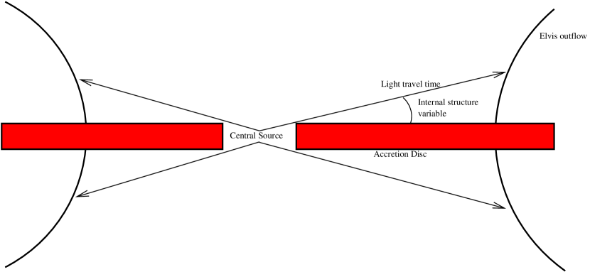
(a) Interpretation of $\epsilon$ for a central source much smaller than the thickness of the accretion disc

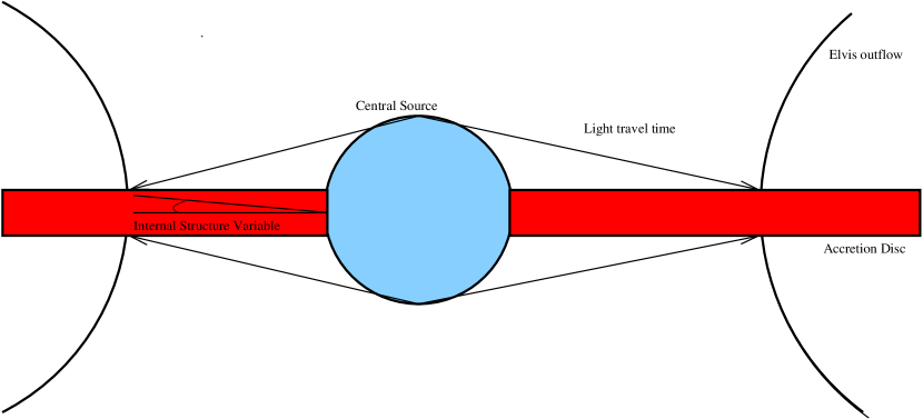
(b) Interpretation of $\epsilon$ if the central source extends above and below the accretion disc

Figure 6: Interpretations of $\epsilon$

An accurate way of discriminating between these two interpretations may be found by analysing the mean reverberation profiles from the four outflow surfaces and producing a relation between the timing of the central reverberation peak and that of the onset of reverberation by a specific outflow surface. The two figures above demonstrate how the timing of reverberation onset is interpreted in the two cases of compact vs extended central source but to discriminate, models must be produced of the expected reverberation profiles for these two cases. Results from [44] would predict the former, as indeed would [31] and [12] and so figure 6a would seem favourable, though analysis of the reverberation profiles will enable a more concrete determination of the meaning of $\epsilon$. Models may then be produced of the expected brightness patterns for differing outflow geometries and compared to the observed light curves to determine the curvature and projection angles of the outflows.

The calculated luminosities may now be compared to the calculated $R_{blr}$ for this sample to determine whether the [17] or [18] relations hold for quasars. Fig. 7 demonstrates that there is absolutely no correlation found for this group of objects. This is not entirely unsurprising as even for nearby AGN both [17] and [18] had enormous scatters in their results, though admittedly not as large as those given here. One important thing to note is that given a predicted factor 200 range in luminosity, one might take [18] as a lower limit on the expected spread, giving a predicted range of $R_{blr}$ of approximately a factor 15. The sensitivity range of this project in $R_{blr}$ is a function of the inclination angle of the quasar but in theory the $R_{blr}$ detectable at zero inclination would be 500 light days with a minimum detectable $R_{blr}$ at this inclination of 50 light days. This factor 10 possible spread of course obtains for any inclination angle giving possibly an infinite spread of $R_{blr}$. For the calculated RMS of 77 light days, the standard deviation is 10.2 light days, 2% of the calculated mean. The probability of NOT finding a factor 15 range of $R_{blr}$ if it exists is therefore less than 1%. Therefore it can be stated to high confidence that this result demonstrates that the [17] and [18] results do not hold for quasars. The failure of [17] for this data set is evident from the fact that it predicts an even larger spread in $R_{blr}$ than [18] which is therefore even less statistically probable from our data. It is possible that this is a failure of the SED of [42], that there are some as-yet unrecognised absorption effects affecting the observations or that the assumption of negligable absorption/re-emission times is incorrect but the more likely explanation would seem to be that no correlation between $R_{blr}$ and luminosity exists for quasars.

Figure 7: Relative luminosities and broad line radii. Absolutely no correlation is seen between $R_{rel}$ (the relative $R_{blr}$) and $L_{rel}$ (the relative luminosity), demonstrating that the [17] and [18] results do not hold for quasars. The error bars are so small that they are contained within the data points.

A calculated average $R_{blr}$ of 544 light days corresponds to $1.4\times 10^{18}cm$, compared to the predicted average of $\sim 10^{18}cm$. The value found here is in remarkable agreement with those previously calculated, made even more surprising by the fact that so few results were available upon which to base a prediction. Many quasar models predict a large variation in quasar properties, see for example [19], so we conclude that quasars and perhaps AGN in general are an incredibly homogeneous population.

7 Conclusions

Brightness records of 57 quasars taken from the MACHO survey in R and V colour filters have been analysed to show the presence of autocorrelation structure consistent with biconic outflowing winds at an average radius of $544\pm 5.2$ light days with an RMS of 74 light days. An internal structure variable of $11.87\pm 0.40^{o}$ was found, with an RMS of $2.9^{o}$. The accuracy of the program designed to determine the timing of the reverberation peaks limited its temporal resolution to 100 days, resulting in the quoted systematic errors in the mean values calculated. With longer-timescale, more regularly sampled data this temporal resolution can be improved - this may also be achieved with more sophisticated computational techniques combined with brightness models not available in this project.

The correlations between radius of the broad emission line region and luminosity found by [17] and [18] for nearby AGN do not appear to hold for quasars. This may be indicative of some time or luminosity evolution of the function as no redshift-independant correlation is found in this data set. If there is some relation it is more likely to be time-evolving since any luminosity dependance would most likely be noticeable in Fig. 7, which it is not.

The presence of reverberation in 57 of the 57 quasars analysed implies that the outflowing wind is a universal structure in quasars - a verifiable result since this structure may be identified in regularly-sampled quasars in other surveys. While it is acknowledged that red noise may yet be responsible for the brightness fluctuations observed, the results are so close to the initial model’s prediction that noise seems an unlikely explanation, especially given the corroborating evidence for the theory [11, 12, 21, 23, 24].

The continuum variability of quasars, though well observed, is still not well understood. The results of this study would suggest that an understanding of these fluctuations can only be found by recognising that several physical processes are at work, of which reverberation is of secondary importance in many cases. It does however appear to be universally present in quasars and possibly in all AGN. Given that quasars are defined observationally by the presence of broad, blue-shifted emission lines, of which outflowing winds are the proposed source, this result is strong support for the [1] model.

8 Future Work

Several phenomena identified in the MACHO quasar light curves remain as yet unexplained.

1. What is the source of the long-term variability of quasars? Is it a random noise process or is there some underlying physical interpretation? It has been suggested that perhaps a relativistic orbiting source of thermal emission near the inner accretion disc edge may be the source of such fluctuation. Modelling of the expected emission from such a source must be undertaken before such a hypothesis can be tested.

2. Why is it that the brightness profile following a dimming event sometimes agrees perfectly with the brightening profile while at other times it is in perfect disagreement? Again, is this a real physical process? Work by [45] on stratified wind models presents a situation where the central object brightening could increase the power of an inner wind, increasing its optical depth and thus shielding outer winds. This would result in negative reverberation. Further investigation may demonstrate a dependance of this effect on whether the central variation is a brightening or fading.

3. What is the mean profile of each reverberation peak? This profile may yield information about the geometry of the outflowing wind, thus enabling constraints to be placed on the physical processes that originate them.

4. Can quasars be identified by reverberation alone? Or perhaps by the long-term variability they exhibit? With surveys such as Pan-STARRS and LSST on the horizon, there is growing interest in devloping a purely photometric method of identifying quasars.

5. LSST and Pan-STARRS will also produce light curves for thousands of quasars which can then be analysed in bulk to produce a higher statistical accuracy for the long-term variability properties of quasars. It is evident that the sampling rate will only be sufficient for reverberation mapping to be performed with LSST and not Pan-STARRS.

6. Is there a time- or luminosity-evolving relation between $R_{blr}$ and luminosity? Comparison of $R_{blr}$, luminosity and redshift may yet shed light on this question.

9 Acknowledgements

I would like to thank Rudy Schild for proposing and supervising this project, Pavlos Protopapas for his instruction in IDL programming, Tsevi Mazeh for his advice on the properties and interpretation of the autocorrelation function and Phil Uttley for discussion and advice on stochastic noise in quasars. This paper utilizes public domain data originally obtained by the MACHO Project, whose work was performed under the joint auspices of the U.S. Department of Energy, National Nuclear Security Administration by the University of California, Lawrence Livermore National Laboratory under contract No. W-7405-Eng-48, the National Science Foundation through the Center for Particle Astrophysics of the University of California under cooperative agreement AST-8809616, and the Mount Stromlo and Siding Spring Observatory, part of the Australian National University.

References

- [1] [1] Elvis, M., ApJ, 545, 63 (2000)
- [2] [2] Matthews, T. & Sandage, A., ApJ, 138, 30 (1963)
- [3] [3] Webb, W. & Malkan, M., ApJ, 540, 652 (2000)
- [4] [4] Ogle, P., PhD Thesis, CalTech (1998)
- [5] [5] Fabian, A. et al., arXiv: 0903.4424 (2009)
- [6] [6] Proga, D., ApJ, 538, 684 (2000)
- [7] [7] Proga, D., Ostriker, J. & Kurosawa, R., ApJ, 676, 101 (2008)
- [8] [8] Antonucci, R., Ann. Rev. Ast. & Ap. 31, 473 (1993)
- [9] [9] Magdis, G. & Papadakis, I., ASPC, 360, 37 (2006)
- [10] [10] Schild, R. & Thomson, D., AJ, 113, 130 (1997)
- [11] [11] Schild, R., AJ, 129, 1225 (2005)
- [12] [12] Vakulik, V. et al., MNRAS, 382, 819 (2007)
- [13] [13] Schild, R., Leiter, D. & Robertson, S., AJ, 135, 947 (2008)
- [14] [14] Lovegrove, J. et al., in preparation (2009)
- [15] [15] Robertson, S. & Leiter, D., in New Developments in Black Hole Research (Nova Science Publishers, New York, 2007) pp1-48
- [16] [16] Robertson, S. & Leiter, D., ApJ, 596, 203 (2003)
- [17] [17] Kaspi, S. et al., ApJ, 629, 61 (2005)
- [18] [18] Bentz, M. et al., arXiv: 0812.2283 (2008)
- [19] [19] Woo, J.-H. & Urry, C. M., ApJ, 579, 530 (2000)
- [20] [20] Schild, R., Leiter, D. & Lovegrove, J., in preparation (2009)
- [21] [21] Pooley, D. et al., ApJ, 661, 19 (2007)
- [22] [22] Shakura, N. & Sunyaev, R., A&A, 24, 337 (1973)
- [23] [23] Peterson, B. et al., Ap J, 425, 622 (1994)
- [24] [24] Richards, G. et al., ApJ, 610, 671 (2004)
- [25] [25] Wyithe, S., Webster, R. & Turner, E., MNRAS, 318, 1120 (2000)
- [26] [26] Kochanek, C., ApJ, 605, 58 (2004)
- [27] [27] Eigenbrod, A. et al., A&A, 490, 933 (2008)
- [28] [28] Trevese, D. et al., ApJ, 433, 494 (1994)
- [29] [29] Hawkins, M., MNRAS, 278, 787 (1996)
- [30] [30] Hawkins, M., ASPC, 360, 23 (2006)
- [31] [31] Colley, W. & Schild, R., ApJ, 594, 97 (2003)
- [32] [32] Hawkins, M., A&A, 462, 581 (2007)
- [33] [33] Schild, R., Lovegrove, J. & Protopapas, P., astro-ph/0902.1160 (2009)
- [34] [34] Uttley, P. et al., PTPS, 155,170 (2004)
- [35] [35] Arevalo, P. et al., MNRAS, 389, 1479 (2008)
- [36] [36] Giveon, U. et al., MNRAS, 306, 637 (1999)
- [37] [37] Rengstorf, A. et al., ApJ, 606, 741 (2004)
- [38] [38] Netzer, H., MNRAS, 279, 429 (1996)
- [39] [39] Botti, I. et al., astro-ph/0805.4664 (2008)
- [40] [40] Alcock, C. et al., PASP, 111, 1539 (1999)
- [41] [41] Geha, M. et al., AJ, 125, 1 (2003)
- [42] [42] Richards, G. et al., astro-ph/0601558 (2006)
- [43] [43] Timmer, J. & Koenig, M., A&A, 300, 707 (1995)
- [44] [44] Schild, R., Leiter, D. & Robertson, S., AJ, 132, 420 (2006)
- [45] [45] Gallagher, S. & Everett, J., ASPC, 373, 305 (2007)