Accounting for the Foreground Contribution to the Dust Emission towards Kepler’s Supernova Remnant.

Abstract

Whether or not supernovae contribute significantly to the overall dust budget is a controversial subject. Submillimetre (submm) observations, sensitive to cold dust, have shown an excess at 450 and 850 $\mu$m in young remnants Cassiopeia A (Cas A) and Kepler. Some of the submm emission from Cas A has been shown to be contaminated by unrelated material along the line of sight. In this paper we explore the emission from material towards Kepler using submm continuum imaging and spectroscopic observations of atomic and molecular gas, via H i, ¹²CO ($J$=2–1) and ¹³CO ($J$=2–1). We detect weak CO emission (peak $T_{\rm A}^{*}$ = 0.2–1 k, 1–2 km s^-1 fwhm) from diffuse, optically thin gas at the locations of some of the submm clumps. The contribution to the submm emission from foreground molecular and atomic clouds is negligible. The revised dust mass for Kepler’s remnant is 0.1–1.2 M_⊙, about half of the quoted values in the original study by Morgan et al. (2003), but still sufficient to explain the origin of dust at high redshifts.

1 Introduction

The conditions following a supernova (SN) explosion are thought to be conducive to the formation of dust: the abundances of heavy elements are high, as is the density; temperatures drop rapidly in the expanding ejecta, quickly reaching levels allowing the sublimation of grain materials. Theoretical estimates predict that type-ii SNe should produce a significant quantity of dust, approximately $\rm 0.3-5\,M_{\odot}$ per star, depending on the metallicity, stellar mass and energy of the explosion (e.g. Todini & Ferrara 2001; Nozawa et al. 2003; Schneider, Ferrara & Salvaterra 2004). Some circumstantial evidence also leads us to believe that SNe should be an important source of dust: first, without SNe there is a dust budget crisis in the Galactic ISM. The dust produced in cool stellar atmospheres of intermediate-mass stars, combined with current predictions for how much dust is destroyed in shocks, yields far less dust than is observed (Jones et al. 1994) in the interstellar medium (ISM). Either another source of dust exists, or dust destruction cannot be as efficient as is widely believed. Second, without SNe and their massive precursors as significant sources of dust, it is difficult to explain the immense dust masses found in submillimetre-selected galaxies and quasars at high redshift (e.g. Smail et al. 1997; Isaak et al. 2002; Eales et al. 2003). There is not sufficient time for dust to form in such large quantities from evolved stars alone (Morgan & Edmunds 2003; Dwek et al. 2007 and references therein).

The signature of warm, freshly-formed dust in Cas A was seen in spectroscopic data by Rho et al. (2008), with reported dust masses in the range 0.02–0.05-M_⊙. Smaller fractions of warm dust have been reported in SN2003gd and Kepler (Sugerman et al. 2006; cf. Meikle et al. 2007; Blair et al. 2007). Spitzer observations of SNRs in the Magellanic Clouds are also consistent with small amounts of dust (e.g. Borkowski et al. 2006; Williams et al. 2006). However, Spitzer is not sensitive to the presence of very cold dust, which peaks at wavelengths longer than 160 $\mu$m. To address the question of whether large quantities of dust are present, we require observations at longer wavelengths in the submm.

The Submillimetre Common User Bolometer Array (SCUBA – Holland et al. 1999) on the James Clerk Maxwell Telescope (JCMT) was used to observe the young Galactic SN remnant (SNR) Cas A (Dunne et al. 2003 – hereafter D03), with large excesses of submm emission detected over and above the extrapolated synchrotron components. This was confirmed by ARCHEOPS (Désert et al. 2008). Because of the high spatial correlation with the X-ray and radio emission, this was interpreted as emission from cold dust associated with the remnant. However, some of the submm emission comes from molecular clouds along the line of sight (Krause et al. 2004; Wilson & Batrla 2005). The high degree of submm polarisation suggests that a significant fraction of dust does originate within the remnant ($\sim\rm 1\,M_{\odot}$, Dunne et al. 2009). We now turn to the only other remnant with a reported excess of submm emission over the extrapolated synchrotron: Kepler. We originally interpreted our SCUBA data as evidence for 0.3–3 $\rm{M_{\odot}}$ of dust associated with the remnant (Morgan et al. 2003 – hereafter M03; Gomez et al. 2007), an order of magnitude higher than those predicted from 160-$\mu$m Spitzer data of Kepler (Blair et al. 2007).

Kepler’s SN has a shell-like structure, $\sim$3 arcmin in diameter. Estimates of its distance, using H i absorption features range from 3.9 to 6 kpc (Reynoso & Goss 1999 – hereafter RG99; Sankrit et al. 2008). Its classification has been controversial (Blair et al. 2007; Reynolds et al. 2007; Sankrit et al. 2008) with evidence pointing towards either a type-ia – the thermonuclear explosion of a low-mass accreting star in a binary system – or a type-ib – the core collapse of a massive star. Reynolds et al. proposed that Kepler’s SN was the result of a thermonuclear explosion in a single 8-M_⊙ star, after roughly 50 Myr of evolution, which would make it pertinent to the issue of the dust budget in the early Universe. Of course, understanding dust formation in SNRs is important regardless of the explosion mechanism: dust formation following type-ia SNe would indicate that type-ii SNe would also be likely dust producers (Clayton et al. 1997; Travaglio et al. 1999). Here, we revisit the submm data and ask how much of the submm emission can be associated with the remnant and how much with material along the line of sight.

In this paper, we recalculate the contribution of synchrotron radiation to the submm emission in Kepler using a radio spectral index map (kindly provided by T. DeLaney). We also present the first high-resolution molecular-line map towards Kepler’s SNR and compare this with archival H i data (RG99). In §2.1 we present details of the observations and data reduction; in §2.2 we investigate the possibility of contamination by line-of-sight gas clouds. In §3 we compare the distribution of the dust and gas. In §3.1 we estimate the dust mass in Kepler with results summarised in §4. Simulations of the effects of the SCUBA chop throw are discussed in Appendix4.

2 Observations and analysis

2.1 Submillimetre continuum observations

The reduction of SCUBA data of Kepler’s remnant at 450 and 850 $\mu$m, using standard routines in the SURF software package (Sandell et al. 2001), was described briefly by M03. The observations were carried out over five different nights during 2001–03 using the jiggle-map mode. The array was chopped to remove sky emission; we chose reference positions using a map of the radio emission as a guide, with a chop throw of 180 arcsec (see Fig. 10). The potential hazards of this observing mode are discussed and simulated in §4. In M03 we presented the synchrotron-subtracted 850-$\mu$m image, obtained by scaling the 5-GHz Very Large Array (VLA) map of Kepler using a constant spectral index, $S_{\nu}\propto\nu^{-0.71}$, that being the mean value reported by DeLaney et al. (2002). We take a different approach here, instead using the spectral index map of DeLaney et al. – their Figure 4 – to produce a more accurate estimate of the synchrotron contribution pixel-by-pixel. The flatter spectral index in the north of the remnant means that more flux has been subtracted from the submm images than in the analysis of M03. The final synchrotron-subtracted submm flux densities are $0.4\pm 0.1$ and $2.8\pm 0.7$ Jy at 850 and 450 $\mu$m, respectively.

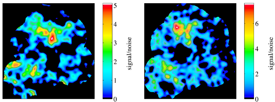
Figure 1: Signal-to-noise submillimetre images of Kepler’s SNR with synchrotron contribution removed. Left: 450 $\mu$m with resolution 16 arcsec and signal-to-noise contours at 2, 3, 4, 5$\sigma$ ($\sigma\sim 46$ mJy beam^-1). Right: 850 $\mu$m with resolution 19 arcsec with contours 3, 4, 5, 6$\sigma$ ($\sigma\sim 8$ mJy beam^-1). The centre of the remnant is at $\rm\alpha_{2000}=17^{h}30^{m}41^{s}.3$, $\rm\delta_{2000}=-21^{\circ}29^{\prime}29^{\prime\prime}$.

The signal-to-noise maps of cold dust at 450 and 850 $\mu$m are shown in Fig. 1, with the synchrotron contribution subtracted using the spectral index image. The noise images were created by randomly generating 1,000 artificial images (Eales et al. 2000). The noise is substantially higher near the edges of the map because these regions received significantly less integration time. At 450 $\mu$m, the centre of the map is also noisy (the array footprint is smaller at 450 $\mu$m than at 850 $\mu$m). The peak signal-to-noise values in these maps are 5$\sigma$ at 450 $\mu$m and 7$\sigma$ at 850 $\mu$m. There are regions of high flux near the edges of the map (particularly in the south-east) but these are also regions of high noise so our confidence in these features is low. Conversly, there are regions of low flux which are not particularly noisy (e.g. in the southern ‘ring’ region of the remnant); our confidence in these features is commensurately higher.

The location of the submm peaks A–J, are marked on the 1.4-GHz map in Fig. 2. This image was constructed using data from the VLA archive (see §2.2.3). Dust clumps A, B, F, I and G all fall within the radius of the shockfront. Most of the emission from cloud E is within the shock also whereas C, D, H, and J lie beyond the X-ray and radio boundaries. Cloud E is located at the position of one of the ‘ears’ in the radio, a region associated with the ejecta but beyond the almost circular shock front. Around 30–40 per cent of the submm flux lies outside the shock front (as defined by the radio observations at 100 arcsec).

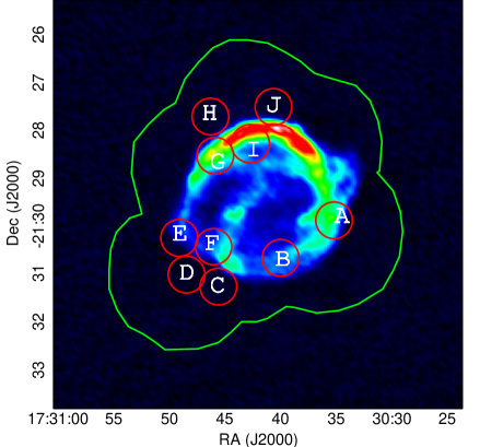
Figure 2: 1.4-GHz VLA image of Kepler’s SNR. The rms noise is 0.6 mJy beam^-1. Submm clumps are labelled A–J with radius, 23 arcsec. The green contour indicates the boundary of the SCUBA observations and the black box indicates the extent of the molecular observations in this work (§ 2.2).

Possible explanations for the submm emission are: (i) dust produced by the supernova remnant or progenitor star; (ii) interstellar material along the line of sight and/or (iii) spurious structure in the SCUBA map – perhaps an artefact of the observing or data processing techniques. These are possibilities we will explore in the remainder of this paper.

2.2 Exploring the possibility of line-of-sight contamination

Does Kepler’s SNR have significant interstellar material along the line of sight that may be contributing to the measured submm fluxes? Kepler’s SNR is approximately 600 pc out of the Galactic Plane ($l\sim\rm 4.5^{\circ}$, $b\sim\rm 6.8^{\circ}$) with extinction and 100-$\mu$m background lower than measured at Cas A by a factor of three (IRAS IRSKY maps – Arendt 1989). A latitude-velocity map of integrated ¹²CO ($J$=1–0) (kindly provided by T. Dame) at the location of Kepler shows that the velocity range of clouds integrated over longitude is confined to $-5<v<5$ km s^-1 (Fig. 3a). Fig. 3b shows the integrated CO emission near Kepler’s SNR (marked by the radio contour in the centre) from the processed Galactic CO survey (Dame et al. 2001). The remnant is within 3^∘ of the $\rho$ Oph cloud complex (distance, 165 pc) which has clouds with line widths ($\Delta v$) up to 100 km s^-1.

2.2.1 ¹²CO($J$=2–1) observations: searching for molecular structures

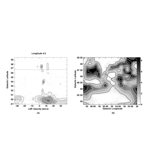
Figure 3: (a) Latitude-velocity map at a longitude of 4.5^∘ from the CO Milky Way Survey (e.g. Dame et al. 2001). Contours show $T_{\rm A}^{*}$ ranging from 0.3 to 4.5 k in steps of 0.6 k. A line at a constant latitude of 6.8^∘ is included to show the location of Kepler’s SNR. The greyscale goes from 0 to 8.5 k, as shown at the right of Fig. 3b. (b) Integrated CO image of the molecular clouds (part of the Ophiuchus complex at 165 pc) in the vicinity of Kepler’s SNR, taken from the Galactic CO data available at http://cfa-www.harvard.edu/mmw/MilkyWaynMolClouds.html. The resolution is 8 arcmin and the integration spans over $-300<v<300$ km s^-1. The contours are at constant $T_{\rm A}^{*}$, ranging from 1 to 9 k in steps of 1 k. The greyscale is indicated to the right of the image. An outer radio continuum contour of Kepler’s SNR with location indicated by the arrow.

In order to quantify the possible contribution from foreground molecular material, we observed Kepler’s SNR in the ¹²CO($J$=2–1) line using the A3 receiver on the JCMT with the Auto-Correlation Spectrometer Imaging System (ACSIS) in double-sideband mode (DSB) (Table 1). The bandwith was 1.8 GHz with 1,904 channels and a velocity coverage of 2,000 km s^-1. We raster-mapped over a region $\rm 8\times 8$ arcmin² with grid points separated by 7 arcsec to avoid smearing in the scan direction (the beam at this wavelength is 20.8 arcsec fwhm). The integration time was 5 s at each point. In this intial dataset, the lines were unresolved. Further high-resolution service observations were obtained to resolve the lines at the location of two CO peaks. The high-resolution data were taken with the same receiver set-up, but with a bandwidth of 250 MHz, 8,192 channels and a velocity coverage of 300 km s^-1. Spectral resolutions and positions are given in Table 1. The spectra were baseline-subtracted with a third-order polynomial and scaled to main beam ($T_{\rm MB}$) temperatures by dividing the antenna temperatures ($T_{\rm A}^{*}$) by the telescope efficiency $\eta_{\rm MB}\sim 0.69$.

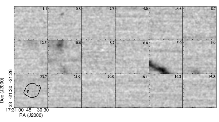
Figure 4: Channel maps of $T_{\rm A}^{*}$ across the ¹²CO ($J$=2–1) transition ranging from $-10$ to 24.6  km s^-1 with velocity width, $\Delta v=1.9$ km s^-1. The images have been smoothed with a 21-arcsec gaussian. The central velocity is labeled on each grid and the negative greyscale ranges from $-0.41$ to 1.2 k km s^-1. Three clouds are detected: to the south of the remnant at velocities 3–5 km s^-1, to the north at velocities 9–11 km s^-1 and a small cloud in the north at velocities 0–2 km s^-1.

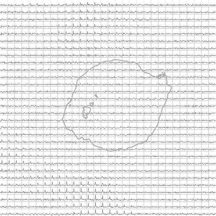
Figure 5: Grid of ¹²CO ($J$=2–1) spectra towards Kepler’s SNR from $-5<v<+15$ km s^-1 across the entire area. The black contour defines the shockfront as estimated from radio observations (Fig. 2). The faint, narrow-line emission from the two molecular clouds in the south and in the north are clearly visible outside the area encompassed by the supernova remnant.

Line	R.A.	Dec.	$t$ (mins.)	Date (2007)	Beam (hpbw)	Spectral resolution	Pos. switch to:
12CO ($J$=2–1)	17:30:42.0	-21:29:35.4	1320	March 08 - April 08	20.8′′	977 kHz, 1.27 km s-1	-426.0′′, +72.0′′
12CO ($J$=2–1)	17:30:45.8	-21:33:10.9	57	June 04	20.8′′	31 kHz, 0.08 km s-1	+163.8′′, +374.1′′
12CO ($J$=2–1)	17:30:46.0	-21:27:23.7	167	June 04	20.8′′	31 kHz, 0.08 km s-1	+161′′, +721.3′′
13CO ($J$=2–1)	17:30:45.8	-21:33:10.9	167	June 04, 08	21.3′′	31 kHz, 0.08 km s-1	+163.8′′, +374.1′′

Table 1: Summary of the CO observations used in this work.

We detect faint, narrow emission corresponding to the radial velocities of the CO and H i emission in the nearby $\rho$ Ophiuchus cloud complex between $-8<v<20$ km s^-1 (de Geus 1992). Channel maps showing the total CO brightness temperature over the range $-7.6<v<20.3$ km s^-1 with velocity intervals of 1.9 km s^-1 are shown in Fig. 4. This range encompasses all of the CO lines detected over the entire velocity coverage. Lines are observed at velocities of $-$1.4, 3.8 and 11.5 km s^-1 with linewidths (fwhm) $\Delta v\leq 0.8$ km s^-1, indicating cold, faint clouds. These lines are narrower than expected for giant molecular clouds, typical interstellar material (GMCs; Solomon, Sanders & Scoville 1979, $\Delta v\sim$4-7 km s^-1), so-called dark clouds and high-Galactic-latitude clouds (Lada et al. 2003). The high-resolution spectra at locations listed in Table 1 were fitted with Gaussian profiles using the SPLAT–VO package (Draper & Taylor 2006) with CO intensities ranging from 0.5-1.4 k km s^-1. It is difficult to ascertain distances to these structures since the Galactic rotation models break down towards the Galactic Centre. Without an estimate of distance to the CO structures, the observed size-velocity dispersion relationship for molecular clouds in the Milky Way (Tsuboi & Miyazaki 1998; Oka et al. 1998) suggests that the CO clouds are smaller than 1 pc across.

We see no evidence for shocked molecular gas which would broaden the lines to average linewidths $\Delta v$$>$15 km s^-1, as seen in the SNRs W28, W44 and W51C (De Noyer 1979; Junkes et al. 1992; Koo & Moon 1997; Seta et al. 1998; Reach, Rho & Jarrett 2005). If an interaction is present, we would expect to observe CO emission peaking at the location of the shock front (e.g. Wilner et al. 1998) and a velocity jump across the outer shock front. Fig. 5 shows the grid of spectra across the entire map, smoothed to a velocity resolution of 3 km s^-1 and restricted to $-5<v<+15\rm\,km\,s^{-1}$ for clarity. The location of the supernova shockfront (defined by the outer radio contour) is overlaid. The molecular clouds detected here lie outside the shock front and line-broadening is not observed in the profiles. We also investigated the velocity gradients across the clouds by integrating in R.A. and declination (Fig. 6). The CO clouds at 4 and 11 km s^-1 line up at a common R.A., spanning 280 arcsec with a velocity range of $\sim$2 km s^-1. The clouds span a similar range in Dec. and velocity in the RA. velocity-position map; the lack of velocity gradient in these images confirms there is no interaction.

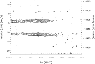
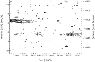
Figure 6: High-resolution ¹²CO ($J$=2–1) spatial-velocity maps of the region surrounding Kepler’s SNR. Top: R.A.-velocity map with contours starting at 0.04 k and incrementing by 0.03 k. Bottom: Dec.-velocity map with contours starting 0.07 k and incrementing by 0.03 k.

2.2.2 ¹³CO($J$=2–1) observations

We observed the brightest ¹²CO($J$=2–1) cloud, at 11 km s^-1, in ¹³CO ($J$=2–1) and detected no emission; the high-resolution spectrum is shown in Fig. 7. The 3 $\sigma$ upper limit can be estimated using $I_{\rm CO}<3\sigma T_{\rm MB}\sqrt{\Delta v\,\delta v}$, where $\delta v$ is the velocity width of the channel and $\Delta v$ is the velocity width of the expected line. We find an upper limit of $I(^{13}{\rm CO})<0.08$ k km s^-1, for a width of 1 km s^-1 (the maximum width detected at the same location in ¹²CO). The lower limit on the brightness ratio $R$ is therefore $I(^{12}{\rm CO})/I(^{13}{\rm CO})>$17. This is larger than those usually found in GMCs where $R\sim 5$ (Solomon et al. 1979).

The optical depth, $\tau^{13}_{\nu}$, is estimated using Eq. 1:

$$\tau_{\nu}=-{\rm ln}\left[1-{T^{13}_{\rm MB}\over{T_{0}}}\left({{1\over{e^{\left(T_{0}/T_{\rm ex}\right)}-1}}}-{{1\over{e^{\left(T_{0}/2.7\right)}-1}}}\right)^{-1}\right]$$ (1)

where $T_{0}$=$h\,\nu/k$. Without further knowledge of the excitation temperature of the gas $T_{\rm ex}$, we assume a nominal value of 15 k (similar to the dust temperatures implied by the 450-/850-$\mu$m flux ratios, M03). The upper limit on the optical depth is $\tau_{\nu}^{13}<8\times 10^{-3}$ for $T_{\rm ex}$=15 k, assuming that $T_{\rm ex}$ is the same for the ¹²CO and ¹³CO molecules. The non-detection of ¹³CO indicates that the ¹²CO emission is optically thin and confirms that we are observing faint emission from a diffuse molecular cloud. Under the assumption that the excitation temperature is the same for both molecules and emission fills the beam, the 3-$\sigma$ upper limit on the optical depth of the ¹²CO emission is $\tau_{\nu}^{12}<0.15$ (Eq. 2).

$${T_{\rm mb}(^{12}{\rm CO})_{\nu}\over{T_{\rm mb}(^{13}{\rm CO})_{\nu}}}={1-\exp{\left(-\tau^{12}_{\nu}\right)}\over{1-\exp\left({-\tau^{13}_{\nu}}\right)}}$$ (2)

The beam-averaged total column density, $N$, can be estimated using the standard assumptions of radiative transfer in local thermodynamic equilibrium (LTE) for an optically thin gas (Thompson & MacDonald 1999):

$$N={3k\over{8\pi^{3}}}{\int T_{\rm MB}{\rm d}v\over{\nu S\mu^{2}g_{\rm I}g_{\rm K}}}Q(T_{\rm ex}){\rm exp}\left({E_{u}\over{kT_{\rm ex}}}\right),$$ (3)

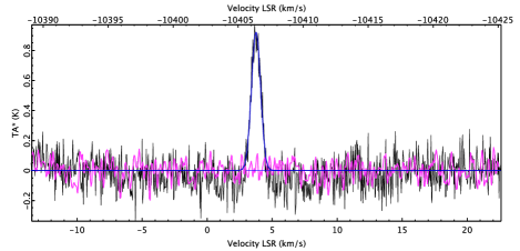
Figure 7: ¹²CO($J$=2–1) high-resolution spectra (black) observed at the location listed in Table 1 over the velocity range $-14<v<23$ km s^-1. The corresponding ¹³CO($J$=2–1) spectra are shown in purple. The peak CO emission is $<$1 with velocity widths $\Delta v<$1 km s^-1.

where $\nu$ is the line frequency, $S$ is the line strength, $\mu$ is the permanent electric dipole moment (in e.s.u), $g_{\rm I}$ and $g_{\rm K}$ are the reduced nuclear spin degeneracy and K-level degeneracy. $E_{\rm u}$ is the energy of the upper level and $Q$ is the partition function of the molecule (with excitation temperature, $T_{\rm ex}$). Values for the constants were obtained from Rohlfs & Wilson (2000) and the Jet Propulsion Laboratory (JPL) database (Pickett et al. 1998). To determine the $\rm H_{2}$ column density, we assume a $\rm{}^{12}CO$ to $\rm H_{2}$ abundance ratio of $\sim 8.5\times 10^{-6}$ (appropriate for diffuse clouds e.g. Liszt 2007; for comparison, the typical values quoted for dense clouds is $8\times 10^{-5}$). The peak column densities of the molecular gas $N(\rm H_{2})$ seen towards Kepler’s remnant estimated from the $\rm{}^{12}CO$ emission are 3.3, 4.4 and 9.1$\times 10^{19}$ cm^-2.

The upper limit on the column density from the ${}^{13}\rm CO$ emission can be estimated using a similar approach to Eq. 3, with an assumed linewidth and excitation temperature for the ¹³CO line set from the observed values for the ¹²CO emission (e.g. Thompson & Macdonald 2003). Assuming a conversion ratio between ¹³CO to $\rm H_{2}$ of $\sim 2\times 10^{-7}$ (e.g. Langer & Penzias 1990), we estimate the $3\,\sigma$ limit on the molecular column density $N({\rm H}_{2})<$$10^{20}$ cm^-2 at the location where we measure both ¹²CO and ¹³CO (i.e. the peak emission in ${}^{12}\rm CO$).

In order to confirm the validity of our LTE analysis we also modeled the ¹²CO line emission with a non-LTE radiative transfer code (van der Tak et al. 2007). The code assumes an isothermal, homogenous medium which fills the telescope beam and solves the radiative transfer equation using the escape probability formulation. We modeled the integrated intensity of the ¹²CO emission for each of the three positions given in Table 1, assuming a kinetic temperature $T_{\rm k}$=15 k and a range of different H₂ densities. The results of our modelling fully confirm our LTE analysis, confirming that the ¹²CO emission is both optically thin and in LTE. Column densities derived by both methods agree within a factor of 3. The radiative transfer models also suggest an upper limit for the H₂ column density of $\sim$10²⁰ cm^-2.

2.2.3 H i observations: searching for atomic structures

To search for atomic foreground features towards Kepler, we have revisited the H i observations reported in RG99, made between 1996 and 1997, with the VLA in its CnB, C and D configurations. The number of spectral channels was 127, centred at 0 km s^-1 (LSR) with a resolution of 1.3 km s^-1. We studied a region of about 25 arcmin $\times$ 25 arcmin centred on Kepler’s SNR. The raw data were downloaded from the VLA public archive and calibrated with the aips package, following standard procedures. The continuum was subtracted in the visibility plane (recall Fig. 2) and the Fourier transform and cleaning of the images was carried out using the miriad data processing package (Sault, Teuben & Wright 1995). A first data cube was constructed using natural weighting. The resolution and sensitivity achieved were slightly improved with respect to those reported in RG99 but the sidelobe level was unacceptable, so a second cube was constructed using uniform weighting which drastically reduced the sidelobes and improved the resolution but degraded the sensitivity.

We constructed an opacity ($\tau$) cube, defined as:

$$\tau=-{\rm ln}\left(1+T_{\rm B}(v)\over T_{\rm c}\right)$$ (4)

where $T_{\rm B}(v)$ is the brightness temperature at velocity $v$ and $T_{\rm c}$ is the continuum emission. To construct the continuum image (Fig. 2), the line-free channels used to determine the spectral baseline were combined in the u,v plane and inverted using uniform weighting. The resulting beam is 9.2 arcsec $\times$ 5.5 arcsec, PA$=$51.6^∘, and sensitivity, 0.6 mJy beam^-1. As originally noted in RG99, the H i emission is uniform in structure, this is confirmed in the opacity cubes and we find no evidence for a correlation of H i structures with the submm emission. Several trials were made to improve the sensitivity by Hanning smoothing the spectral profiles and convolving the images to larger beams, with little success. Addition of single dish data from the LAB survey (Hartmann & Burton 1997; Kalberla et al. 2005) to the images did not add evidence of a correlation.

Using the VLA H i and single-dish data we can estimate the column density of atomic gas at the location of the submm clumps:

$$N=1.82\times 10^{18}\,\int T{\rm d}v$$ (5)

where $v$ is the velocity (in km s^-1). Integrating over the velocity range in which large-scale H i features are seen ($-10<v<22$ km s^-1), we detect small variations in emission on the H i map, with minimum and maximum column densities of 0.6-0.9$\times 10^{21}$ cm^-2. The atomic gas density is at least an order of magnitude higher than the molecular density estimated from the CO. The chopping procedure employed in the submm observations of Kepler’s SNR can not produce the submm structures from chopping on-off these small variations, indeed chopping would have removed any emission associated with the H i as was seen in Cas A (Wilson & Bartla 2005).

3 Comparing the Gas and Dust Towards Kepler

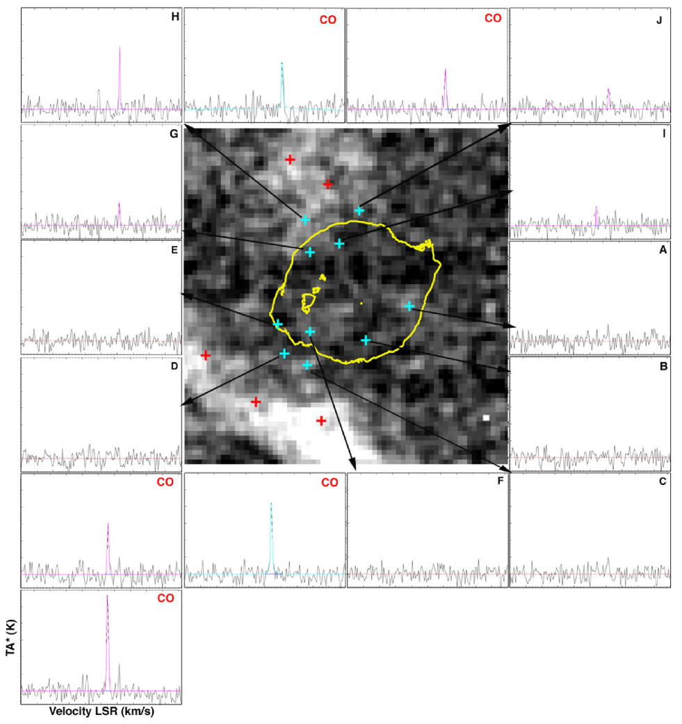
Figure 8: Integrated ¹²CO($J$=2–1) emission towards Kepler’s SNR over the velocity range $-$200–200 km s^-1 smoothed by a 3 km s^-1 Gaussian. The crosses indicate regions where spectra were taken across the CO clouds and the remnant. Cyan crosses show the locations of the submm clumps A–F, red crosses are positions chosen with strong CO emission for comparison. The integrated spectra from apertures at the locations of the submm clumps and at the CO clouds are shown alongside over the velocity range $-50<v<50$ km s^-1 (unsmoothed). The greyscale ranges from $-$1.4 to 1.9 k km s^-1.

Name	Coords		$T_{\rm peak}$	$v_{\rm c}$	fwhm	r.m.s.	$I({\rm CO})$	$N(^{12}{\rm CO})$	$N({\rm H}_{2})$	$S_{\rm 850}$
	$\Delta$ R.A.	$\Delta$ Dec.	k	(km s-1)	(km s-1)	k	(k km s-1)	($10^{14}$ cm-2)	($10^{19}$ cm-2)	(mJy)
CO S	+221.9	+95.9	0.63	4.06	1.14	0.05	1.12	6.0	7.1	..
			0.51	11.17	0.46	0.05	0.25	1.1	1.3	..
CO S	+146.3	+82.7	0.67	4.05	1.10	0.05	0.78	4.3	4.9	..
CO S	+51.1	+192.5	0.46	4.30	1.00	0.06	0.49	2.7	3.1	..
CO N	+96.9	$-$190.9	0.34	11.48	1.17	0.05	0.42	2.2	2.7	..
CO N	+47.6	$-$153.5	1.14	11.12	0.18	0.06	0.81	4.4	5.1	..
A	$-$83.3	+23.3	0.14	11.4	0.96	0.05	0.16	8.6	10.2	28.8 $\pm$ 3.5
B	$-$17.5	+71.8	..	..	..	0.05	$\leq$0.15	$\leq$0.8	$\leq$1.0	23.0 $\pm$ 2.9
C	+69.3	+110.3	0.13	11.21	1.59	0.05	0.22	1.2	1.5	41.5 $\pm$ 4.6
D	+101.5	+93.3	..	..	..	0.05	$\leq$ 0.15	$\leq$0.8	$\leq$1.0	45.8 $\pm$ 4.9
E	+109.9	+47.3	..	..	..	0.05	$\leq$0.15	$\leq$0.8	$\leq$1.0	62.1 $\pm$ 6.6
F	+94.5	+58.3	..	..	..	0.06	$\leq$0.18	$\leq$1.0	$\leq$1.1	21.8 $\pm$ 2.7
G	+65.1	$-$57.0	0.20	11.27	0.87	0.05	0.19	10.2	1.2	30.6 $\pm$ 3.6
H	+70.7	$-$104.7	0.55	$-$1.59	0.48	0.05	0.28	1.6	1.8	63.8 $\pm$ 6.7
			0.55	11.36	0.76	0.05	0.42	2.2	2.7	..
I	+21.7	$-$71.7	0.23	11.71	0.68	0.05	0.20	1.1	1.2	31.4 $\pm$ 3.3
J	$-$7.7	$-$118.7	0.27	11.70	0.72	0.05	0.21	1.1	1.3	33.5 $\pm$ 3.8

Table 2: Properties of the detected ¹²CO ($J$=2–1) line emission towards Kepler’s SNR. Columns show (1) name (2) offset coordinates from centre in arcsec ($\rm RA=17^{h}30^{m}41^{s}.3$ and $\rm Dec.=-21^{\circ}29^{\prime}29^{\prime\prime}$ where postive R.A. and Dec. indicates a move to the East and South); (3) peak $T_{\rm MB}$ (4) central velocity (5) velocity width (fwhm) (6) integrated intensity (7) rms (8) and (9) column densities of CO and H₂ gas estimated using Eq. 3 and (10) the submm flux measured in the apertures A–J after synchrotron subtraction. Errors are estimated using the procedure outlined in Dunne & Eales (2001).

The high resolution ¹²CO ($J$=2–1) map integrated over the velocity range $-200<v<200$ km s^-1, is shown in Fig. 8 with the outer contour of the radio image overlaid. The map has been smoothed with a 21-arcsec Gaussian. Cyan crosses indicate the submm dust clumps, A–J; red crosses indicate CO peaks. Spectra at each of these locations were extracted; where CO was detected, the lines were fitted with Gaussian profiles with the derived properties given in Table 2. Also listed in Table 2 are the fluxes in the submm clumps, A–J, determined by placing an aperture of radius 23 arcsec on the synchrotron-subtracted 850-$\mu$m image. The sum of the fluxes in these apertures is 0.38 Jy (cf. 0.58 Jy in M03). The submm clumps outside the remnant are located on average, in regions of higher CO emission than those inside the remnant, however a significant fraction of the submm flux comes from clumps where there is no, or little CO emission. Comparing the distribution of the CO and submm emission spatially, we can see that molecular clouds are observed at the location of submm clumps G and H (combined flux of 94 mJy) and fainter emission at clumps A, C, I and J (combined submm flux 135 mJy). We do not detect CO emission at the locations of the submm clumps B, D, E and F (combined submm flux 153 mJy).

The CO column densities towards these clumps is a better indicator of the quantity of line-of-sight emission. At apertures A–J, these range from $<$10¹⁴–10¹⁵ cm^-2 with molecular gas densities $10^{19}$–$10^{20}$ cm^-2. The gas column densities estimated from the submm fluxes range from $10^{21}$ to $10^{22}$ cm^-2 (with gas-to-dust ratio of 160); as confirmed by the column densities estimated from the (lower-resolution) 100$\mu$m IRIS maps (Miville-Deschênes & Lagache 2005). This a factor of 10-100 times higher than that estimated from the CO data. If the submm clumps were related to the same molecular gas as traced by the foreground CO emission, the conversion ratio $N\rm(H_{2})/CO$ in these clumps would have to be less than $10^{-7}$ which is far lower than the values ($>$$10^{-5}$) expected for clouds with densities of $10^{21}$–$10^{22}$ cm^-2 (e.g. Listz 2007). Conversely, using the appropriate conversion factor for the molecular gas densities estimated from the submm clumps, we would expect to observe CO column densities $N(\rm CO)>$$10^{16}$–$10^{17}$ cm^-2 at the location of the submm emission. This suggests that the molecular gas contribution to the submm emission towards Kepler is negligible, even where CO is co-spatial with the submm clumps on the sky.

Are there any physical effects that could result in our underestimating the column density of the gas? In dense molecular cores, CO and other molecules may become depleted from the gas phase by freezing out onto the surfaces of dust grains (e.g. Redman et al. 2002). The timescale for molecular freezeout is tightly correlated to the gas density and only becomes significant for H₂ densities $>$10⁵ cm^-3 (Caselli et al. 1999). If this were the case then we would expect to see evidence for higher gas densities in the form of higher optical depths and the presence of rarer isotopologues of CO. The properties of the ¹²CO emission that we have detected are strongly suggestive of diffuse clouds in which molecular depletion does not play a significant role in controlling the abundance of CO.

In diffuse molecular clouds, the CO abundance depends on the overall H₂ column density (Liszt et al 2007), likely due to the increased UV photodissociation rates for CO in low density gas (van Dishoeck & Black 1988). However, in order to match the column densities indicated by the submm emission, the density of the gas would increase to a point where photodissociation is largely unimportant except at the exterior of the cloud. The CO to H₂ abundance ratio for gas with an H₂ column density of 10²¹–10²² is close to that expected for a dark molecular cloud and not consistent with the column densities of CO that we observe. We thus conclude that neither depletion or photodissociation are likely to have a significant effect upon our derived column densities.

3.1 The revised dust mass in Kepler’s remnant

The IR–submm spectral energy distribution (SED) of Kepler’s SNR, using the synchrotron-subtracted submm fluxes is shown in Fig. 9. We fit a two-component modified blackbody to the SED which is the sum of two modified Planck functions, each with a characteristic temperature, $T_{w}$ and $T_{c}$ (Eq. 6):

$$S_{\nu}=N_{w}\times\nu^{\beta}B(\nu,T_{w})+N_{c}\times\nu^{\beta}B(\nu,T_{c})$$ (6)

where $N_{w}$ and $N_{c}$ represent the relative masses in the warm and cold component, $B(\nu,T)$ is the Planck function and $\beta$ is the dust emissivity index. The model was fitted to the SED (constrained by the 12-$\mu$m flux) and the resulting parameters ($N_{w}$, $N_{c}$, $T_{w}$, $T_{c}$, $\beta$) which gave the minimal $\chi^{2}$ were found.

The solid curve shows the fit to the SED with $S_{100}=5.6\pm 1.4$ Jy (the average from Arendt 1989 and Saken, Fesen & Shull 1992) whilst the dot-dashed curve fits the SED with the lower 100-$\mu$m flux of 2.9 Jy (estimated from pointed observations, Braun 1987). The higher 100-$\mu$m flux predicts the lower dust mass for the SED model. Both fits include the recent Spitzer fluxes at 24 and 70 $\mu$m (Blair et al. 2007) but the 160 $\mu$m upper limit is not included in the fit due to uncertainties with the background at this wavelength. Neither fit to the IR data alone would provide evidence for a cold dust component, highlighting the importance of accurate submm fluxes when estimating the dust mass. Note that the SED is equally well fit in both cases and to distinguish between the two, more accurate fluxes are needed around the peak of the cold emission at 200–400 $\mu$m.

In addition to using the range of IRAS 100-$\mu$m fluxes in the literature, we also applied a bootstrap analysis to our SED fitting to determine the errors on the model. The photometry measurements were perturbed according to the errors at each wavelength (using the higher 100-$\mu$m flux which produces the lowest mass). The new fluxes were fitted in the same way, the SED parameters and dust masses recorded, with the procedure repeated 3,000 times. The median results along with errors (estimated from the 68 per cent confidence intervals) are listed in Table 3.

Figure 9: IR–submm SED for Kepler’s SNR, comparing the best fits with two different 100-$\mu$m fluxes, including Spitzer data and submm points (this work). The solid line represents the best fit with $S_{100}\sim 5.9\pm 1.4$ Jy. The dot-dashed curve represents the fit to the lower 100-$\mu$m flux, $2.9\pm 0.9$ Jy. The upper limit shown by the arrow is the total integrated flux obtained from Spitzer at 160 $\mu$m (Blair et al. 2007).

The dust mass is calculated from the SED model using Eq. 7.

$$M_{d}={S_{850}D^{2}\over{\kappa_{850}}}\times\left[{N_{w}\over{B({\rm 850}~{}\mu{\rm m},T_{w})}}+{N_{c}\over{B({\rm 850}~{}\mu{\rm m},T_{c})}}\right]$$ (7)

where $\kappa_{850}$ is the dust absorption coefficient and the distance, $D$ is taken to be the lower published limit of 3.9 kpc (Sankrit et al. 2008). To determine the dust mass, we take two extreme values for $\kappa$: (i) $\kappa_{850}=0.07$ m² kg^-1, typical quoted value for grains in the diffuse interstellar medium (D03 and references therein) and (ii) $\kappa_{850}=0.7$ m² kg^-1, as required for the submm polarimetry observations of Cas A (Dunne et al. 2009). This is similar to the values ($\sim 0.4$ m² kg^-1) predicted by the supernova dust model in Bianchi & Schneider (2007). The range of dust masses obtained from the SED model (Eqs. 6 & 7) is therefore 0.1–1.2 $\rm M_{\odot}$ depending on $\kappa$. Note that $\kappa$ is the largest source of error when estimating the mass of dust from IR/submm emission.

Bootstrap parameters			Dust mass (M⊙)
$\beta$	$T_{\rm w}$ (k)	$T_{\rm c}$ (k)	$\kappa_{1}\rm\,(m^{2}\,kg^{-1})$	$\kappa_{2}\rm\,(m^{2}\,kg^{-1})$
$2.0\pm 0.2$	$88^{+6}_{-4}$	$16\pm 1$	$0.12^{+0.02}_{-0.03}$	$1.2^{+0.18}_{-0.30}$

Table 3: The best-fit parameters for Kepler’s SNR estimated from the bootstrap technique. The dust mass is the median of the distribution from the bootstrap technique with the error quoted from the 68 per cent confidence interval. $\kappa_{1}=0.7\rm\,m^{2}\,kg^{-1}$ (appropriate for SNR dust, Dunne et al. 2009) and $\kappa_{2}=0.07\rm\,m^{2}\,kg^{-1}$ (typical ISM values) which gives the maximum mass.

4 Conclusions

We have presented information on the reduction and analysis of SCUBA submm data of Kepler’s SNR including a more accurate subtraction of the synchrotron component. The residual fluxes are slightly lower than those previously reported. We find that the ring-like structure seen in the submm cannot be reproduced by chopping on-off large scale structures. Large-scale FIR/submm imaging is crucial to determine whether the observed submm structures are unique to the SNR, or are common in this region. Such observations will soon be possible with SCUBA-2 and the Herschel Space Observatory.

We investigated whether foreground molecular or atomic structures could be responsible for the submm emission concluding that:

• There are three molecular clouds in the vicinity of Kepler’s SNR, located on the periphery of the remnant in the north and south-east and extending further out in the south. The clouds are faint and cold ($T_{\rm A}^{*}$ $<$1 k, $\Delta v<1$ km s^-1). Molecular gas column densities towards the remnant are estimated to be $\leq$$10^{20}$ cm^-2.

• ¹³CO line emission is not detected at the locations of the peak ¹²CO emission. The 3-$\sigma$ upper limit on the molecular column density is $<$$10^{20}$ cm^-2 indicating that the clouds are diffuse and optically thin. This is confirmed with an independent analysis.

• The column densities estimated from the submm are 10–100 times higher than the column densities estimated from the molecular gas. This difference cannot be explained by reasonable variations in the conversion factor between CO and $\rm H_{2}$ emission nor can it be explained by depletion or photodissociation effects.

The molecular contribution to the submm emission towards Kepler’s remnant is therefore negligible. The dust mass associated with the remnant ranges from 0.1–1.2 $\rm M_{\odot}$, depending on the absorption coefficient. This value is 100 times larger than seen by Spitzer and concurs with the results for Cas A (Dunne et al. 2009) that supernovae are significant sources of dust.

Appendix A Spurious structure due to chopping?

The observing technique used when obtaining the original SCUBA data (§2.1) could affect the apparent distribution of submm emission around Kepler’s SNR if we had chopped onto structure unrelated to the remnant. We modeled the effect of chopping onto interstellar structures not associated with the remnant using the chop positions and throws chosen for Kepler (Fig. 10). The simulations were performed by sampling the sky model at the appropriate on-off source chop locations, white noise was added before reconstructing the on-source flux measurements from the three different chop/nod positions. We included different input models of the sky, here we discuss the results using (i) large scale interstellar submm structures (with the CO emission as a guide, Fig. 11a) and (ii) large scale interstellar submm structures including a SNR ring-like structure at the location of Kepler (based on the radio image, Fig. 11d).

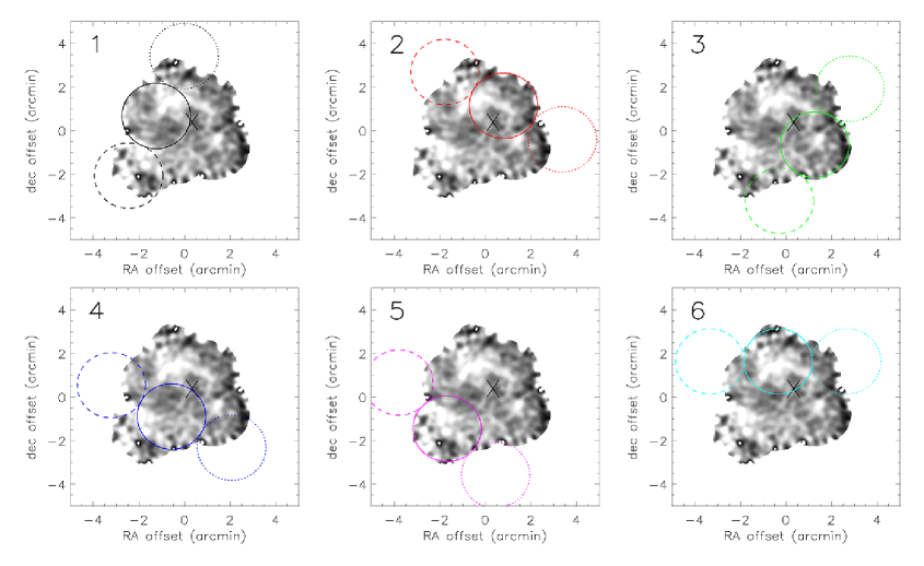
Figure 10: The individual six SCUBA jiggle maps and corresponding chop positions. The greyscale image is the total 850-$\mu$m signal-to-noise image.

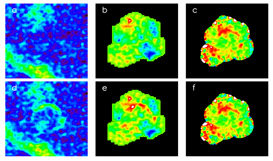
Figure 11: Simulating the SCUBA maps: the input maps with foreground CO used as an example of large scale structures surrounding Kepler (a) combined with the radio SNR (d). The results are given in b and e. Panels c and f show the original SCUBA (S/N) map at 850 $\mu$m for reference.

The results are shown in Figs. 11b and 11e along with the original SCUBA data in the same colour scale (c and f). We see some spurious structure in the simulated output for case (i) as a result of chopping on to the bright extended structure in the south seen in the input sky. The effect of this chop is diminished when averaged over the two off-source chop positions (jiggles three and five). The strong ring-like emission structure seen in the SCUBA data (c) is not reproduced in the simulation, suggesting that the ring cannot be a result of chopping on or off large scale background structures. This is supported by the output from case (ii) which includes a SNR model in the input (e). The ring-like structure survives after chopping on-off the larger surrounding structures. We conclude that the emission in the SCUBA map is due to a ring-like source of submm radiation and is not an artifact of the observing technique.

References

- [1] Arendt R.G., 1989, ApJS, 70, 189
- [2] Bianchi S., Schneider R., 2007, MNRAS, 378, 973
- [3] Blair W.P., Ghavamian P., Long K.S., Williams B.J., Borkowski K.J., Reynolds S.P., Sankrit R., 2007, ApJ, 662, 998
- [4] Borkowski K.J., Kazimierz J., Williams B.J., Reynolds S.P., Blair W.P., Ghavamian P., Sankrit R., Hendrick S.P., 2006, ApJ, 642, L141
- [5] Braun R., 1987, A & A, 171, 233
- [6] Caselli, P., Walmsley, C. M., Tafalla, M., Dore, L., & Myers, P. C. 1999, ApJ, 523, L165
- [7] Clayton D.D., Arnett D., Kane J., Meyer B.S., 1997, AJ, 486, 824
- [8] Dame T., Hartmann D., Thaddeus P., 2001, ApJ, 547, 792
- [9] de Geus E., 1992, A & A, 262, 258
- [10] DeLaney T., Koralesky B., Rudnick L., Dickel J.R., 2002, ApJ, 580, 914
- [11] DeNoyer L.K., 1979, ApJ, 232, L165
- [12] Désert F.-X., Macías-Pérez J.F., Mayet F., Giardino G., Renault C., Aumont J., Benoît A., Bernard J.-Ph, Ponthiey N., Tristram M., 2008, A & A, 481, 411
- [13] Draper P., Taylor M.B., 2006, A Spectral Analysis Tool, Starlink User Note 214
- [14] Dunne L., Eales S., 2001, MNRAS, 327, 697
- [15] Dunne L., Eales S., Ivison R.J., Morgan H., Edmunds M., 2003, Nature, 424, 285 [D03]
- [16] Dunne L., Maddox S.J., Ivison R.J., Rudnick L.R., DeLaney T.M., Matthews B.C., Crowe C.M., Gomez H.L., Eales S.A., Dye S., 2009, MNRAS, 320
- [17] Dwek E., Galliano F., Jones A.P., 2007, ApJ, 662, 927
- [18] Eales S., Lilly S., Webb T., Dunne L., Gear W., Clements D., Yun M., 2000, AJ, 120, 2244
- [19] Eales S., Bertold F., Ivison R.J., Carilli C.L., Dunne L., Owen F., 2003, MNRAS, 344, 169
- [20] Gomez H.L., Eales S.A., Dunne L., 2007, IJAsB, 6, 159
- [21] Hartmann D., Burton W. B., 1997, Atlas of Galactic Neutral Hydrogen, Cambridge University Press, UK
- [22] Holland W.S. et al., 1999, MNRAS, 303, 659
- [23] Isaak K., Priddey R.S., McMahon R.G., Omont A., Peroux C., Sharp R.G., Witthington S., 2002, MNRAS, 329, 149
- [24] Jones A.P., Tielens A.G.G.M., Hollenbach D.J., McKee C.F., 1994, ApJ, 433, 797
- [25] Junkes N., Furst E., Reich W., 1992, A & ASS, 96, 1
- [26] Koo B-C., Moon D-S., 1997, ApJ, 485, 263
- [27] Krause O., Birkmann S.M., Reike G., Lemke D., Klaas U., Hines D.C., Gordon K.D., 2004, Nature, 432, 596
- [28] Lada C.J., Bergin E.A., Alves João-F., Huard T.L., 2003, ApJ, 586, L286
- [29] Langer W.D., Penzias A.A., 1990, ApJ, 357, 477
- [30] Liszt H.S., 2007, A & A, 476, 291
- [31] Margulis M., Lada C.J., 1985, ApJ, 299, 925
- [32] Meikle W.P.S., Mattila S., Pastorello A., Gerardy C.L., Kotak R., Sollerman J., Van Dyk S.D., Farrah D., 2007, ApJ, 665, 608
- [33] Miville-Deschênes M.-A., Lagache G., 2005, ApJSS, 157, 302
- [34] Morgan H.L., Edmunds M.G, 2003, MNRAS, 343, 427
- [35] Morgan H.L., Dunne L., Eales S., Ivison R.J., Edmunds M.G., 2003, ApJ, 597, L33 [M03]
- [36] Nozawa T., Kozasa T., Umeda H., Maeda K., Nomoto K., 2003, ApJ, 598, 785
- [37] Pickett H. M., Poynter R. L., Cohen E. A., Delitsky M. L., Pearson J. C., M ller H. S. P., 1998, J. Quant. Spectrosc. Radiat. Transfer, 60, 883
- [38] Reach W.T., Rho J., Jarett T.H., 2005, ApJ, 618, 297
- [39] Redman, M. P., Rawlings, J. M. C., Nutter, D. J., Ward-Thompson, D., & Williams, D. A. 2002, MNRAS, 337, L17
- [40] Reynolds S., Borkowski K.J., Hwang U., Hughes J.P., Badenes C., Laming J.M., Blondin J.M., 2007, ApJ, 668, L135
- [41] Reynoso E.M., Goss W.M., 1999, AJ, 118, 926 [RG99]
- [42] Rho J., Kozasa T., Reach W.T., Smith J.D., Rudnick L., DeLaney T., Ennis J.A., Gomez H., Tappe A., 2008, ApJ, 673, 271
- [43] Rohlfs K., Wilson T. L., 2000, Tools of Radio Astronomy, 3rd Edition, Springer-Verlag, Berlin
- [44] Saken J.M., Fesen R.A., Shull J.M., 1992, ApJS, 81, 715
- [45] Sandell G., Jessop N., Jenness T., 2001, SCUBA Map Reduction Cookbook, Starlink Cookbook 11.2
- [46] Sankrit R., Blair W.P., Frattare L.M., Rudnick L., DeLaney T., Harrus, I.M., Ennis J.A., 2008, AJ, 135, 538
- [47] Sault R. J., Teuben P. J., Wright M. C. H., 1995, in Astronomical Data Analysis Software and Systems IV, eds Shaw R.A., Payne H.E., Hayes J.J.E., ASP, 77, 433, San Francisco
- [48] Schneider R., Ferrara A., Salvaterra R., 2004, MNRAS, 351, 1379
- [49] Seta M, Hasegawa T, Dame T.M., Sakamoto S., Ok T., Handa T., Hayashi M., Morin J-I., Sora K., Usuda K.S., 1998, ApJ, 505, 286
- [50] Smail I., Ivison R.J., Blain A.W, 1997, ApJ, 490, L5
- [51] Solomon P.M., Sanders D.B., Scoville N.Z., 1979, ApJ, 232 L89
- [52] Sugerman, B.E.K., Ercolano B., Barlow M.J., Tielens A.G.G.M., Clayton G.C., Zijlstra, A.A., Meixner, M., Speck, A., 2006, Science, 313, 196
- [53] Thompson M.A., MacDonald G.H., 1999, A & AS, 135, 531
- [54] Thompson M.A., MacDonald G.H., 2003, A & AS, 407, 237
- [55] Todini P., Ferrara A., 2001, MNRAS, 325, 726
- [56] Travaglio C., Gallino R., Amari S., Zinner E., Woosley S., Lewis R.S., 1999, ApJ, 510, 325
- [57] van der Tak, F. F. S., Black, J. H., Schöier, F. L., Jansen, D. J., & van Dishoeck, E. F. 2007, A & A, 468, 627
- [58] van Dishoeck E.F., Black J.H., 1988, ApJ, 334, 771
- [59] Williams B.J. et al., 2006, ApJ, 652, L33
- [60] Wilner D.J., Reynolds S.P., Moffett D.A., 1998, AJ, 115, 247
- [61] Wilson T.L., Batrla W., 2005, A & A, 430, 561