Abstract

The process $p\bar{p}\to\Lambda_{c}^{+}\bar{\Lambda}{}_{c}^{-}$ is investigated within the handbag approach. It is shown that the dominant dynamical mechanism, characterized by the partonic subprocess $u\bar{u}\to c\bar{c}$, factorizes in the sense that only the subprocess contains highly virtual partons, a gluon to lowest order of perturbative QCD, while the hadronic matrix elements embody only soft scales and can be parameterized in terms of helicity flip and non-flip generalized parton distributions. Modelling these parton distributions by overlaps of light-cone wave functions for the involved baryons we are able to predict cross sections and spin correlation parameters for the process of interest.

1 Introduction

The FAIR project at GSI with the HESR antiproton program will offer ideal possibilities to study exclusive channels in $p\bar{p}$ annihilation. The energy of the antiproton beam suffices to produce pairs of heavy baryons, as for instance $\Lambda_{c}^{+}\bar{\Lambda}{}_{c}^{-}$, in proton-antiproton collisions. Prerequisite for the measurement of such processes is, however, that their cross sections are sufficiently large. The purpose of this work is to estimate the cross section for the reaction $p\bar{p}\to\Lambda_{c}^{+}\bar{\Lambda}{}_{c}^{-}$. This estimate is based on a generalization of the, so-called, “handbag approach”, which has been developed for deeply virtual electroproduction of photons and mesons [1]. It has been firmly shown that the amplitudes for these processes are described by convolutions of hard subprocess kernels and, so-called, “generalized parton distributions” (GPDs), which encode the soft, non-perturbative physics. A second class of hard exclusive reactions to which the handbag approach can be applied to, is formed by wide-angle reactions. The hard scale for these reactions, necessary to justify factorization into hard and soft physics, is provided by the momentum transfer from the incoming to the outgoing hadron or, in other words, by large Mandelstam variables $-t$ and $-u$, instead of the photon virtuality. Although, in contrast to deeply virtual processes, rigorous proofs do not exist, arguments for the dominance of the handbag contribution have been given in some cases [2, 3, 4].

Along the lines of argumentation for wide-angle Compton scattering [2] we demonstrate that, under the assumption of restricted parton virtualities and transverse momenta, the $p\bar{p}\to\Lambda_{c}^{+}\bar{\Lambda}{}_{c}^{-}$ amplitudes factorize into hard subprocesses and moments of the $u\!\to\!c$ transition GPDs. Owing to the relatively heavy charm quarks (with mass $m_{c}$), the process possesses the large intrinsic scale $4m_{c}^{2}\simeq 6.3\,\,{\rm GeV}^{2}$ to which the momentum transfer adds. The large intrinsic scale leads to the highly welcome consequence that large $-t$ and $-u$ are not required as, say, for wide-angle Compton scattering. Therefore the arguments for factorization of the $p\bar{p}\to\Lambda_{c}^{+}\bar{\Lambda}{}_{c}^{-}$ amplitude already hold for small scattering angles.

It is to be stressed that the process of interest has already been investigated long time ago [5] in an approach that bears resemblance to the handbag one. As compared to [5] the progress achieved here manifests itself in the more solid theoretical basis. The normalization of the cross section is now determined for given GPDs and not fixed by symmetry arguments as in [5]. Moreover, the complicated structure of the proton which is described in terms of eight GPDs, can be easily taken into account in the handbag approach and therefore the spin dependence of the process $p\bar{p}\to\Lambda_{c}^{+}\bar{\Lambda}{}_{c}^{-}$ can readily be treated.

The plan of the paper is the following: The arguments for factorization and the principle structure of the handbag contribution are presented in Sect. 2. In Sect. 3 the amplitudes of the process $p\bar{p}\to\Lambda_{c}^{+}\bar{\Lambda}{}_{c}^{-}$ are discussed while the subprocess amplitudes are given in Sect. 3.1. Various models for the GPDs are presented in Sect. 4 and predictions for observables are discussed in Sect. 5. The summary is given in Sect. 6. In two appendices various kinematical formulas and the properties of the transition GPDs are compiled.

2 Factorization

2.1 The basic idea

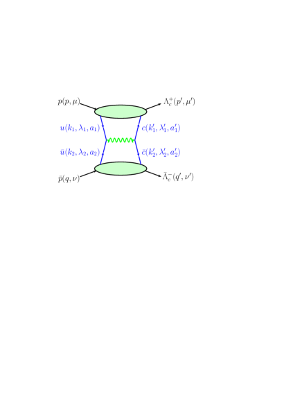
Figure 1: The handbag contribution to the process $p\bar{p}\to\Lambda_{c}^{+}\bar{\Lambda}_{c}^{-}$. The momenta and helicities of the baryons and quarks as well as the colors of the latter, are also specified.

We assume that the graph shown in Fig. 1 dominates the process of interest for Mandelstam $s$ well above the kinematical threshold and in the forward scattering hemisphere. We are going to show in this section that the baryons emit and re-absorb soft partons, i.e. quarks that are almost on-shell and move almost collinear with their parent baryon. In other words, the contribution from the graph shown in Fig. 1 factorizes into a hard partonic subprocess and soft hadronic matrix elements. The arguments for factorization go along the same lines as for wide-angle Compton scattering [2], except that here we have to consider the double handbag and we have to take care of the unequal mass kinematics . For the $p\to\Lambda_{c}^{+}$ transition a $u$-quark is to be emitted and a $c$-quark reabsorbed; the valence quark content is to be changed. The emission of a light quark other than the $u$ one from the proton does not lead to a $\Lambda_{c}$ baryon in the final state. Intrinsic charm would allow for subprocesses like

$$\bar{c}\,\bar{u}\,\to\,\bar{u}\,\bar{c}\,.$$ (1)

This is a higher Fock-state contribution which is expected to be suppressed by general arguments. Moreover, according to present PDF analyses, e.g. [7, 8], the charm content of the proton is tiny. Even at a scale of, say, $25\,\,{\rm GeV}^{2}$ it only amounts to about $10^{-3}$ of the $u$-quark content at $x\simeq 0.6$. Thus, we merely have to take into account the subprocess

$$u\bar{u}\to c\bar{c}\,.$$ (2)

This subprocess goes along with $p\to\Lambda_{c}^{+}$ transition matrix elements which, as we are going to show below, can be parameterized by $u\to c$ GPDs. One may also think of time-like matrix elements or GPDs representing $p\bar{p}\to{u}\bar{u}$ and ${c}\bar{c}\to\Lambda_{c}^{+}\bar{\Lambda}{}_{c}^{-}$ transitions. Such time-like GPDs have been employed in the analysis of wide-angle time-like processes as, for instance, two-photon annihilation into a pair of hadrons [9, 10, 11]. To lowest order of QCD the subprocess is mediated by one-gluon exchange which evidently forbids the time-like reaction mechanism by color conservation to this order of accuracy. It is, however, allowed to higher orders of QCD although, beyond representing an $\alpha_{s}$ correction, expected to be smaller than the mechanism depicted in Fig. 1 since the $p\to\Lambda_{c}^{+}$ transitions seem to favored over the time-like ones. We therefore do not consider the time-like mechanism.

A $u\to c$ transition GPD is a function of three variables, a momentum fraction $\bar{x}$ defined by the ratio of light-cone plus components of the average parton and baryon momenta (see Fig. 1)

$$\bar{x}_{1}\,=\,\frac{k_{1}^{+}+k_{1}^{\prime+}}{p^{+}+p^{\prime+}}\,,$$ (3)

the skewness parameter

$$\xi\,=\,\frac{p^{+}-p^{\prime+}}{p^{+}+p^{\prime+}}\,,$$ (4)

and Mandelstam $t$. Analogous definitions hold for the antibaryon vertex. The $u\to c$ transition GPDs are expected to exhibit a maximum which becomes more pronounced as the mass of the heavy quark increases. The position of the peak is approximately at

$$x_{0}\,=\,m_{c}/M\,=\,1-\epsilon/M\,,$$ (5)

for not too large $-t$. The width of the peak shrinks with increasing mass. For standard values of the charm quark mass [12]

$$m_{c}\,=\,(1.27\textstyle{+0.07\atop-0.11})\,\,{\rm GeV}\,,$$ (6)

$x_{0}$ is about 0.5 - 0.6. The parameter $\epsilon$ is the difference between the hadron and the heavy quark mass and has a value of about $0.6-1.0\,\,{\rm GeV}$. In the formal limit of $m_{c}\to\infty$ $x_{0}$ tends to 1 according to the heavy quark effective theory (HQET) [13]. This expected property of the transition GPDs parallels the theoretically expected and experimentally confirmed behavior of heavy quark fragmentation functions, in particular $c\to\Lambda_{c}^{+}$ (see [14, 15]) and is also analogous to the behavior of light-cone wave functions (LCWFs) and distribution amplitudes for heavy baryons [16, 17]). The $x$ dependence of the transition GPD is to be contrasted with wide-angle Compton scattering [2] and the zero-skewness GPD analysis [18] where the GPDs exhibit a behavior similar to the one expected for the $u\to c$ transition only for $-t\gg 1\,{\rm GeV}^{2}$.

Some kinematical details of our process of interest are compiled in App. A. As for Compton scattering we work in a symmetric frame with the baryon momenta as specified in (88) and assume that the virtualities of all the partons the baryons are made of are smaller then $\Lambda^{2}$ where $\Lambda$ is a typical hadronic scale of order $1\,\,{\rm GeV}$. Of course, the virtualities of the charm and anticharm quark respect the relation $\mid k^{\prime 2}-m_{c}^{2}\mid\leq\Lambda^{2}$. We further assume that all parton transverse momenta satisfy the restrictions:

$$\tilde{\bf k}_{\perp}^{2}{}_{i}/\tilde{x}_{i}\raisebox{-4.0pt}{$\,\stackrel{{\scriptstyle\textstyle<}}{{\sim}}\,$}\Lambda^{2}\,,\qquad\hat{\bf k}_{\perp}^{\prime\,2}{}_{i}/\hat{x}^{\prime}_{i}\raisebox{-4.0pt}{$\,\stackrel{{\scriptstyle\textstyle<}}{{\sim}}\,$}\Lambda^{2}\,,$$ (7)

where, for the ease of legibility, we have not distinguished between the parton momenta from the upper and lower vertex. The bounds for the transverse momenta are assumed to hold in hadron frames in which the respective hadron moves along the 3-direction (the tilde characterizes momenta in the hadron-in frame, the hat those in the hadron-out frame). These hadron frames are reached by transverse boosts, cf. e.g. [19]. This is a transformation that leaves the plus component of any momentum vector $a$ unchanged. It involves a parameter $b^{+}$ and a transverse vector ${\bf b}_{\perp}$ and is defined by

$$[a^{+},a^{-},{\bf a}_{\perp}]\longrightarrow\left[a^{+},a^{-}-\frac{{\bf a}_{\perp}\cdot{\bf b}_{\perp}}{b^{+}}+\frac{a^{+}{\bf b}_{\perp}^{2}}{2(b^{+})^{2}},{\bf a}_{\perp}-\frac{a^{+}}{b^{+}}{\bf b}_{\perp}\right]\,.$$ (8)

The corresponding transformation for antibaryons requires transverse boosts that leave the minus components of the momenta unchanged. In the following we discuss the baryon vertex in detail. All the arguments and results given below do hold for the antibaryon vertex analogously.

The active parton momenta are parameterized as

$$k_{1}\,=\,[x_{1}{p}^{+},k_{1}^{-},{\bf k}_{1\perp}]\,,\qquad k_{1}^{\prime}\,=\,[x_{1}^{\prime}{p}^{\prime+},k_{1}^{\prime-},{\bf k}_{1\perp}^{\prime}]\,.$$ (9)

The individual momentum fractions $x_{1}$ and $x_{1}^{\prime}$ are related to $\bar{x}_{1}$ and the skewness by

$$x_{1}\,=\,\frac{\bar{x}_{1}+\xi}{1+\xi}\,,\qquad x_{1}^{\prime}\,=\,\frac{\bar{x}_{1}-\xi}{1-\xi}\,.$$ (10)

Transforming the parton momenta (9) to the respective hadron-in or hadron-out frame by the transverse boost (8), we find

$$\tilde{k}_{1}\,=\,[x_{1}{p}^{+},\ldots,{\bf k}_{1\perp}+x_{1}{\bf\Delta}_{\perp}/2]\,,\qquad\hat{k}_{1}^{\prime}\,=\,[x_{1}^{\prime}{p}^{\prime+},\ldots,{\bf k}_{1\perp}^{\prime}-x_{1}^{\prime}{\bf\Delta}_{\perp}/2]\,.$$ (11)

For convenience let us assume that there is only one spectator . The generalization to an arbitrary number of spectators is straightforward but tedious. As is characteristic of any parton approach the momenta of the active parton ($k_{1}$ and $k_{1}^{\prime}$) and the spectator ($k_{s}$ and $k_{s}^{\prime}$) sum up to the parent baryon’s momentum. Hence,

$${\bf k}_{\perp}{}_{s}\,=\,-{\bf\Delta}_{\perp}/2-{\bf k}_{1\perp}\,,\qquad x_{s}\,=\,1-x_{1}\,,$$ (12)

and analogously for $k^{\prime}_{s}$. The spectator condition $k^{\phantom{\prime}}_{s}=k^{\prime}_{s}$ leads to $x_{1}^{\prime}(1-\xi)=x_{1}(1+\xi)-2\xi$ and ${\bf k}_{1\perp}^{\prime}={\bf\Delta}_{\perp}+{\bf k}_{1\perp}$. Transforming also the spectator momenta to the respective hadron frames and using the supposition (7), we can write

$$2\Lambda^{2}\geq\tilde{k}^{2}_{\perp s}/\tilde{x}_{s}+\hat{k}^{\prime\,2}_{\perp s}/\hat{x}^{\prime}_{s}\,=\,\frac{1-\bar{x}_{1}}{1-\xi^{2}}\Delta_{\perp}^{2}/2+\frac{2}{1-\bar{x}_{1}}({\bf k}_{1\perp}+{\bf\Delta}_{\perp}/2)^{2}\,.$$ (13)

Each term in this inequality is positive. Therefore, each one is separately bounded by $2\Lambda^{2}$. The inequality for the second term on the right hand side of (7) compels ${\bf k}_{1\perp}\simeq-{\bf\Delta}_{\perp}/2$ for large $m_{c}$. This result can be approximated by the more convenient form

$${\bf k}_{1\perp}\simeq-x_{1}{\bf\Delta}_{\perp}/2\quad{\rm for}\quad m_{c}\to\infty$$ (14)

since the relevant values of $\bar{x}_{1}$ are about $x_{0}$, i.e. large. Analogously, one obtains ${\bf k}_{1\perp}^{\prime}\simeq x_{1}^{\prime}{\bf\Delta}_{\perp}/2$. Approximating $\bar{x}_{1}$ by the peak position $x_{0}$, we find from the first term in (13)

$$\Delta_{\perp}^{2}\raisebox{-4.0pt}{$\,\stackrel{{\scriptstyle\textstyle<}}{{\sim}}\,$}4\,\frac{\Lambda^{2}}{1-x_{0}}(1-\xi^{2})\,.$$ (15)

In the formal limit of $m_{c}\to\infty$ where $x_{0}$ tends to 1, this inequality is respected for any fixed value of $\Delta_{\perp}^{2}$. Even for a realistic value of about 0.6 for $x_{0}$ the range of allowed values for $\Delta_{\perp}^{2}$ is sufficiently large for our purpose of studying the process $p\bar{p}\to\Lambda_{c}^{+}\bar{\Lambda}_{c}^{-}$. Finally, the assumption of bounded virtualities, $\mid k_{1}^{2}\mid\leq\Lambda^{2}$ and $\mid k_{1}^{\prime 2}-m_{c}^{2}\mid\leq\Lambda^{2}$, provides $k_{1}^{-}\simeq x_{1}p^{-}$ and an analogous result for $k_{1}^{\prime\,-}$.

The above considerations lead to the following approximation of the momenta of the active partons (9) (${k}_{1}^{(\prime)+}=x_{1}^{(\prime)+}p^{(\prime)+}$, $\;{k}_{2}^{(\prime)-}=x_{2}^{(\prime)-}q^{(\prime)-}$):

$$k_{1}\to\bar{k}_{1} = \left[\;{k}_{1}^{+}\,,\,\frac{x_{1}^{2}\Delta_{\perp}^{2}}{8{k}_{1}^{+}}\,,-\frac{1}{2}x_{1}{\bf\Delta}_{\perp}\right]\,,$$

$$k^{\prime}_{1}\rightarrow\bar{k}^{\prime}_{1} = \left[\;{k}_{1}^{\prime+},\frac{m_{c}^{2}+x_{1}^{\prime 2}\Delta_{\perp}^{2}/4}{2{k}_{1}^{\prime+}},\frac{1}{2}x_{1}^{\prime}{\bf\Delta}_{\perp}\right],$$

$$k_{2}\rightarrow\bar{k}_{2} = \left[\;\frac{x_{2}^{2}\Delta_{\perp}^{2}}{8{k}_{2}^{-}}\,,\,{k}_{2}^{-}\,,\phantom{-}\frac{1}{2}x_{2}{\bf\Delta}_{\perp}\right],$$

$$k^{\prime}_{2}\rightarrow\bar{k}^{\prime}_{2} = \left[\frac{m_{c}^{2}+x_{2}^{\prime 2}\Delta_{\perp}^{2}/4}{2{k}_{2}^{\prime-}},{k}_{2}^{\prime-},-\frac{1}{2}x_{2}^{\prime}{\bf\Delta}_{\perp}\right].$$ (16)

We introduce the subscripts 1 and 2 in order to distinguish the partons from the $p\to\Lambda_{c}^{+}$ and the $\bar{p}\to\bar{\Lambda}{}_{c}^{-}$ vertex. It is to be emphasized that the parton momenta in this approximation are on-shell and lie in the scattering plane formed by the baryon momenta.

2.2 Calculation of the double handbag

The amplitude for the hadron-hadron scattering process obviously reads,

$${\cal M} = \sum_{\rm a_{i}^{(\prime)},\,\alpha_{i}^{(\prime)}}\int d^{4}k_{1}^{\mathrm{av}}\theta(k_{1}^{\mathrm{av}+})\int\frac{d^{4}z_{1}}{(2\pi)^{4}}e^{ik_{1}^{\mathrm{av}}z_{1}}\int d^{4}k_{2}^{\mathrm{av}}\theta(k_{2}^{\mathrm{av}-})\int\frac{d^{4}z_{2}}{(2\pi)^{4}}e^{ik_{2}^{\mathrm{av}}z_{2}}$$ (17)

$$\times \langle p^{\prime}\mu^{\prime}|T\bar{\Psi}^{c}_{a^{\prime}_{1}\alpha^{\prime}_{1}}(-z_{1}/2)\Psi^{u}_{a_{1}\alpha_{1}}(z_{1}/2)|p\mu\rangle\;\widetilde{H}_{a_{i}^{(\prime)}\alpha^{(\prime)}_{i}}(k_{1}^{(\prime)},k_{2}^{(\prime)})\;$$

$$\times \langle q^{\prime}\nu^{\prime}|T\bar{\Psi}^{u}_{a_{2}\alpha_{2}}(z_{2}/2)\Psi^{c}_{a^{\prime}_{2}\alpha^{\prime}_{2}}(-z_{2}/2)|q\nu\rangle,$$

where we have used $k_{i}^{\mathrm{av}}:=(k_{i}+k_{i}^{\prime})/2$, $(k_{1}-k_{1}^{\prime})=(p-p^{\prime})$, and $(k_{2}-k_{2}^{\prime})=(q-q^{\prime})$. It is understood that the proton emits a parton with momentum $k_{1}$, helicity $\lambda_{1}$ and color $a_{1}$ (cf. Fig. 1). It undergoes a hard scattering with a corresponding antiparton ($k_{2}$, $\lambda_{2}$, $a_{2}$) emitted from the antiproton. The scattered partons, characterized by $k^{\prime}_{1}$, $\lambda^{\prime}_{1}$, $a^{\prime}_{1}$ and $k^{\prime}_{2}$, $\lambda^{\prime}_{2}$, $a^{\prime}_{2}$, are reabsorbed by the remainders of the proton or antiproton and form the $\Lambda_{c}^{+}$ or $\bar{\Lambda}{}_{c}^{-}$, respectively. The labels $\alpha^{(\prime)}_{i}$ are spinor labels. For the ease of writing we will omit the color and spinor labels in the following wherever this can be done without loss of unambiguity. The active $u$ and $\bar{u}$ quarks are treated as massless quarks. We have not to consider an antiquark contribution in the above baryon matrix elements as is necessary in Compton scattering [2]. The quarks in (2) are associated with the $p\to\Lambda_{c}^{+}$ vertex, the antiquarks with the $\bar{p}\to\bar{\Lambda}{}_{c}^{-}$ one.

Since the parton-parton scattering is dominated by a large scale, the heavy quark mass, we can neglect the variation of transverse and minus (plus) components of $k_{i}$ and $k^{\prime}_{i}$ in the hard scattering kernel $\widetilde{H}$ and replace the parton momenta by the on-shell vectors $\bar{k}_{i}^{(\prime)}$ (16). With this replacement of the parton momenta the integrations over $k_{1}^{\mathrm{av}-}$, $k_{2}^{\mathrm{av}+}$ and ${\bf k}_{\perp}{}_{i}^{\mathrm{av}}\,,i=1,2\,,$ can be performed explicitly

$$\int d^{4}k_{1}^{\mathrm{av}}\theta(k_{1}^{\mathrm{av}+})\int\frac{d^{4}z_{1}}{(2\pi)^{4}}e^{ik_{1}^{\mathrm{av}}z_{1}}\int d^{4}k_{2}^{\mathrm{av}}\theta(k_{2}^{\mathrm{av}-})\int\frac{d^{4}z_{2}}{(2\pi)^{4}}e^{ik_{2}^{\mathrm{av}}z_{2}}f(\bar{k}_{1},z_{1},\bar{k}_{2},z_{2})$$

$$=\int dk_{1}^{\mathrm{av}+}\theta(k_{1}^{\mathrm{av}+})\int\frac{dz_{1}^{-}}{2\pi}e^{ik_{1}^{\mathrm{av}+}z_{1}^{-}}\int dk_{2}^{\mathrm{av}-}\theta(k_{2}^{\mathrm{av}-})\int\frac{dz_{2}^{+}}{2\pi}e^{ik_{2}^{\mathrm{av}-}z_{2}^{+}}f(\bar{k}_{1},\bar{z}_{1},\bar{k}_{2},\bar{z}_{2})\,.$$

(18)

We see that the relative distance of the fields in the matrix elements is forced on the light-cone, $\bar{z}_{1}=[0,z_{1}^{-},{\bf 0}_{\perp}]$ and $\bar{z}_{2}=[z_{1}^{+},0,{\bf 0}_{\perp}]$. After this the time-ordering of the fields can be dropped [20].

To show that the plus components indeed dominate the scattering we use the fact that the proton-parton amplitudes, described by the soft matrix elements, can be written as the amplitude for a (anti) proton with momentum $p$ ($q$) emitting the active parton with momentum $\bar{k}_{1}(\bar{k}_{2})$ and a number of on-shell spectators times the corresponding conjugate amplitude for momenta $p^{\prime}(q^{\prime})$ and $\bar{k}^{\prime}_{1}(\bar{k}^{\prime}_{2})$, summed over all spectator configurations; this corresponds to inserting a complete set of intermediate states between the quark and the antiquark fields in the matrix elements.

Using the technique of transverse boosts, we can transform to a frame where $\bar{k}_{1}$ has zero transverse and minus components:

$$\bar{k}_{1}\,=\,[{k}_{1}^{+},0,{\bf 0}_{\perp}]\,.$$ (19)

Using the general result

$$\frac{1}{2}(\gamma^{-}\gamma^{+}+\gamma^{+}\gamma^{-})=1\,,$$ (20)

and the energy projector for quarks 

$$\sum_{\lambda_{1}}u(\bar{k}_{1},\lambda_{1})\bar{u}(\bar{k}_{1},\lambda_{1})\,=\,\bar{k}_{1}\cdot\gamma\,=\,k_{1}^{+}\gamma^{-}\,,$$ (21)

we can write

$$\Psi^{u}(z_{1}/2) = \frac{1}{2}(\gamma^{-}\gamma^{+}+\gamma^{+}\gamma^{-})\Psi^{u}(z_{1}/2)\,=\,\frac{1}{2{k}_{1}^{+}}\sum_{\lambda_{1}}\left[u(\bar{k}_{1},\lambda_{1})\left(\bar{u}(\bar{k}_{1},\lambda_{1})\gamma^{+}\Psi^{u}(z_{1}/2)\right)\right.$$ (22)

$$+ \left.\gamma^{+}u(\bar{k}_{1},\lambda_{1})\left(\bar{u}(\bar{k}_{1},\lambda_{1})\Psi^{u}(z_{1}/2)\right)\right]\,.$$

Due to the central assumption of restricted parton virtualities and transverse momenta (7) there are large plus components at the proton-parton vertex but no large kinematical invariant. Because of this the first term in (22) dominates over the second one and the latter can be neglected. Since a transverse boost leaves the plus component of any vector unchanged, (22) holds in the overall symmetric frame too. Similar considerations for the outgoing partons run into complications with the quark mass. A transverse boost to a frame where $\bar{k}^{\prime}_{1}$ has no transverse component, leads to

$$\bar{k}^{\prime}_{1}\longrightarrow\left[{k}^{\prime+}_{1},\frac{m_{c}^{2}}{2{k}_{1}^{\prime+}},{\bf 0}_{\perp}\right]\,,$$ (23)

with a non-vanishing minus component due to the finite charm-quark mass. The energy projector reads

$$\sum_{\lambda^{\prime}_{1}}u(\bar{k}^{\prime}_{1},\lambda^{\prime}_{1})\bar{u}(\bar{k}^{\prime}_{1},\lambda^{\prime}_{1})\,=\,\bar{k}^{\prime}_{1}\cdot\gamma+m_{c}\,=\,{k}_{1}^{\prime+}\gamma^{-}+\frac{m_{c}^{2}}{2{k}_{1}^{\prime+}}\gamma^{+}+m_{c}$$ (24)

in that frame. For the charm field we can therefore write (with $(\gamma^{+})^{2}=0$)

$$\Psi^{c}(-z_{1}/2) = \frac{1}{2{k}_{1}^{\prime+}}\sum_{\lambda^{\prime}_{1}}\left[u(\bar{k}^{\prime}_{1},\lambda^{\prime}_{1})\left(\bar{u}(\bar{k}^{\prime}_{1},\lambda^{\prime}_{1})\gamma^{+}\Psi^{c}(-z_{1}/2)\right)\right.$$ (25)

$$+ \left.\gamma^{+}\Big{\{}u(\bar{k}^{\prime}_{1},\lambda^{\prime})(\bar{u}(\bar{k}^{\prime}_{1},\lambda^{\prime}_{1})\Psi^{c}_{a^{\prime}_{1}}(-z_{1}/2))-2m_{c}\Psi^{c}(-z_{1}/2)\Big{\}}\right]\,.$$

Using the plane-wave decomposition of the charm-quark field it can be shown that the term within curly brackets vanishes identically if it is applied to a $\Lambda_{c}^{+}$ Fock state in which the charm quark carries momentum $\bar{k}^{\prime}_{1}$. But these are just the states we need in the sequel to describe the absorption of the charm quark, that leaves the hard scattering process with momentum $\bar{k}^{\prime}_{1}$, by the $\Lambda_{c}^{+}$. We therefore conclude again that the first term in (24) dominates over the one within square brackets so that the latter can be neglected. In the overall symmetric frame this term is small as well and we have

$$\Psi^{c}(-z_{1}/2)\,=\,\frac{1}{2{k}_{1}^{\prime+}}\sum_{\lambda^{\prime}_{1}}u(\bar{k}^{\prime}_{1},\lambda^{\prime}_{1})\left(\bar{u}(\bar{k}^{\prime}_{1},\lambda^{\prime}_{1})\gamma^{+}\Psi^{c}(-z_{1}/2)\right)\,.$$ (26)

Employing the light-cone spinors we can write for the helicity non-flip and flip configuration at the $p\to\Lambda_{c}^{+}$ vertex in the symmetric frame

$$\frac{\bar{u}(\bar{k}^{\prime}_{1},\lambda_{1})\gamma^{+}u(\bar{k}_{1},\lambda_{1})}{2\sqrt{{k}^{+}_{1}k_{1}^{\prime+}}} = 1\,,$$

$$\frac{\bar{u}(\bar{k}^{\prime}_{1},-\lambda_{1})\imath\sigma^{+j}u(\bar{k}_{1},\lambda_{1})}{2\sqrt{k^{+}_{1}k_{1}^{\prime+}}} = \imath(2\lambda_{1}\imath)^{j}\,,$$ (27)

where $j=1,2$ and

$$\sigma^{\pm j}\,=\,\imath\gamma^{\pm}\gamma^{j}\,.$$ (28)

Of course, analogous expressions hold for the antiparticle spinors (with an additional minus sign). The helicity projector for the light quarks reads

$$u(\bar{k}_{1},\lambda_{1})\bar{u}(\bar{k}_{1},\lambda_{1})\,=\,\bar{k}_{1}\cdot\gamma(1-2\lambda_{1}\gamma_{5})/2\,.$$ (29)

On the other hand, for the charm quark we have

$$u(\bar{k}^{\prime}_{1},\lambda^{\prime}_{1})\bar{u}(\bar{k}^{\prime}_{1},\lambda^{\prime}_{1})\,=\,\Big{[}\bar{k}^{\prime}_{1}\cdot\gamma+m_{c}\Big{]}(1+\gamma_{5}S_{1}\cdot\gamma)/2\,,$$ (30)

where the covariant spin vector $S_{1}$ reads

$$S_{1}\,=\,\frac{2\lambda^{\prime}_{1}}{m_{c}}\,\big{[}\bar{k}^{\prime}_{1}-\frac{m_{c}^{2}}{{k}_{1}^{\prime+}}\,n^{-}\big{]}\,.$$ (31)

Here, $n^{-}\,=\,[0,1,{\bf 0}_{\perp}]$ is a unit vector. In the limit $m_{c}\to 0$ the spin projector (30) turns into the usual helicity projector.

Now we can simplify the products of quark fields occurring in (17). In fact, forming the product of the first terms in (22) and (25) and inserting (27) between the two terms involving $\gamma^{+}$, one obtains after a little algebra

$$\bar{\Psi}^{c}_{\alpha^{\prime}_{1}}(-z_{1}/2)\,\Psi^{u}_{\alpha_{1}}(z_{1}/2) = \frac{1}{4k^{+}_{1}k^{\prime+}_{1}}\sum_{\lambda_{1}\lambda^{\prime}_{1}}\Big{(}\bar{\Psi}^{c}(-z_{1}/2)\,\gamma^{+}u(\bar{k}^{\prime}_{1},\lambda^{\prime}_{1})\Big{)}$$

$$\times \Big{(}\bar{u}(\bar{k}_{1},\lambda_{1})\gamma^{+}\Psi^{u}(z_{1}/2)\Big{)}\bar{u}_{\alpha^{\prime}_{1}}(\bar{k}^{\prime}_{1},\lambda^{\prime}_{1})u_{\alpha_{1}}(\bar{k}_{1},\lambda_{1})$$

$$\longrightarrow\hskip 68.28383pt \frac{1}{2\sqrt{k^{+}_{1}k^{\prime+}_{1}}}\sum_{\lambda_{1}}\left\{\bar{\Psi}^{c}(-z_{1}/2)\,\gamma^{+}\frac{1+2\lambda_{1}\gamma_{5}}{2}\Psi^{u}(z_{1}/2)\bar{u}_{\alpha^{\prime}_{1}}(\bar{k}^{\prime}_{1},\lambda_{1})u_{\alpha_{1}}(\bar{k}_{1},\lambda_{1})\right.$$ (32)

$$-\left.\imath(-2\lambda_{1}\imath)^{j}\bar{\Psi}^{c}(-z_{1}/2)\,\imath\sigma^{+j}\frac{1+2\lambda_{1}\gamma_{5}}{2}\Psi^{u}(z_{1}/2)\bar{u}_{\alpha^{\prime}_{1}}(\bar{k}^{\prime}_{1},-\lambda_{1})u_{\alpha_{1}}(\bar{k}_{1},\lambda_{1})\right\}\,.\hskip 36.42035pt$$

The quark-mass and the transverse-momentum terms drop out since they always come with products of two $\gamma^{+}$ matrices. Analogously one finds for the $\bar{p}\to\bar{\Lambda}{}_{c}^{-}$ vertex

$$\bar{\Psi}^{u}_{\alpha_{2}}(z_{2}/2)\,\Psi^{c}_{\alpha^{\prime}_{2}}(-z_{2}/2) = -\frac{1}{2\sqrt{k^{-}_{2}k^{\prime-}_{2}}}\sum_{\lambda_{2}}$$ (33)

$$\times\left\{\bar{\Psi}^{u}(z_{2}/2)\,\gamma^{-}\frac{1-2\lambda_{2}\gamma_{5}}{2}\Psi^{c}(-z_{2}/2)\bar{v}_{\alpha_{2}}(\bar{k}_{2},\lambda_{2})v_{\alpha^{\prime}_{2}}(\bar{k}^{\prime}_{2},\lambda_{2})\right.$$

$$-\left.\imath(-2\lambda_{2}\imath)^{j}\bar{\Psi}^{u}(z_{2}/2)\,\imath\sigma^{-j}\frac{1+2\lambda_{2}\gamma_{5}}{2}\Psi^{c}(-z_{2}/2)\bar{v}_{\alpha_{2}}(\bar{k}_{2},\lambda_{2})v_{\alpha^{\prime}_{2}}(\bar{k}^{\prime}_{2},-\lambda_{2})\right\}.$$

Combining now (17), (18), (32) and (33) and using $\lambda_{2}=-\lambda_{1}$, a property of the subprocess amplitude which follows from the fact that massless quarks do not flip their helicities in interactions with photons and/or gluons, one arrives at

$${\cal M} = -\int dk_{1}^{\mathrm{av}+}\theta(k_{1}^{\mathrm{av}+})\int\frac{dz_{1}^{-}}{2\pi}e^{ik_{1}^{\mathrm{av}+}z_{1}^{-}}\int dk_{2}^{\mathrm{av}-}\theta(k_{2}^{\mathrm{av}-})\int\frac{dz_{2}^{+}}{2\pi}e^{ik_{2}^{\mathrm{av}-}z_{2}^{+}}\frac{1}{4\sqrt{k_{1}^{+}k_{1}^{\prime+}k_{2}^{-}k_{2}^{\prime-}}}$$ (34)

$$\times \sum_{\lambda_{1}}\left\{\langle p^{\prime}\mu^{\prime}\mid\bar{\Psi}^{c}(-\bar{z}_{1}/2)\gamma^{+}\frac{1+2\lambda_{1}\gamma_{5}}{2}\Psi^{u}(\bar{z}_{1}/2)\mid p\mu\rangle\,\right.$$

$$\times \left.\langle q^{\prime}\nu^{\prime}\mid\bar{\Psi}^{u}(\bar{z}_{2}/2)\gamma^{-}\frac{1+2\lambda_{1}\gamma_{5}}{2}\Psi^{c}(-\bar{z}_{2}/2)\mid q\nu\rangle\,H_{\lambda_{1}-\lambda_{1},\lambda_{1}-\lambda_{1}}(\bar{k}_{1},\bar{k}_{2})\right.$$

$$- \left.\langle p^{\prime}\mu^{\prime}\mid\bar{\Psi}^{c}(-\bar{z}_{1}/2)\imath\sigma^{+j}\frac{1+2\lambda_{1}\gamma_{5}}{2}\Psi^{u}(\bar{z}_{1}/2)\mid p\mu\rangle\,\right.$$

$$\times \left.\langle q^{\prime}\nu^{\prime}\mid\bar{\Psi}^{u}(\bar{z}_{2}/2)\imath\sigma^{-j}\frac{1-2\lambda_{1}\gamma_{5}}{2}\Psi^{c}(-\bar{z}_{2}/2)\mid q\nu\rangle\,H_{-\lambda_{1}\lambda_{1},\lambda_{1}-\lambda_{1}}(\bar{k}_{1},\bar{k}_{2})\right.$$

$$- \left.\imath(2\lambda_{1}\imath)^{j}\langle p^{\prime}\mu^{\prime}\mid\bar{\Psi}^{c}(-\bar{z}_{1}/2)\gamma^{+}\frac{1+2\lambda_{1}\gamma_{5}}{2}\Psi^{u}(\bar{z}_{1}/2)\mid p\mu\rangle\,\right.$$

$$\times \left.\langle q^{\prime}\nu^{\prime}\mid\bar{\Psi}^{u}(\bar{z}_{2}/2)\sigma^{-j}\frac{1-2\lambda_{1}\gamma_{5}}{2}\Psi^{c}(-\bar{z}_{2}/2)\mid q\nu\rangle\,H_{\lambda_{1}\lambda_{1},\lambda_{1}-\lambda_{1}}(\bar{k}_{1},\bar{k}_{2})\right.$$

$$- \left.\imath(-2\lambda_{1}\imath)^{j}\langle p^{\prime}\mu^{\prime}\mid\bar{\Psi}^{c}(-\bar{z}_{1}/2)\sigma^{+j}\frac{1+2\lambda_{1}\gamma_{5}}{2}\Psi^{u}(\bar{z}_{1}/2)\mid p\mu\rangle\,\right.$$

$$\times \left.\langle q^{\prime}\nu^{\prime}\mid\bar{\Psi}^{u}(\bar{z}_{2}/2)\gamma^{-}\frac{1+2\lambda_{1}\gamma_{5}}{2}\Psi^{c}(-\bar{z}_{2}/2)\mid q\nu\rangle\,H_{-\lambda_{1}-\lambda_{1},\lambda_{1}-\lambda_{1}}(\bar{k}_{1},\bar{k}_{2})\right\}\,.$$

The subprocess amplitudes are defined by

$$H_{\lambda_{1}^{\prime}\lambda_{2}^{\prime},\lambda_{1}\lambda_{2}}(\bar{k_{1}},\bar{k_{2}})\,=\,\bar{v}(\bar{k}_{2},\lambda_{2})\bar{u}(\bar{k}^{\prime}_{1},\lambda^{\prime}_{1})\widetilde{H}(\bar{k}_{1}^{(\prime)},\bar{k}_{2}^{(\prime)})v(\bar{k}^{\prime}_{2},\lambda_{2}^{\prime})u(\bar{k}_{1},\lambda_{1})\,,$$ (35)

where the hard scattering kernel $\widetilde{H}(\bar{k}_{1}^{(\prime)},\bar{k}_{2}^{(\prime)})$ has to be evaluated for parton momenta as given in (16).

2.3 Peaking approximation, GPDs and form factors

According to our discussion in Sect.2.1 we set $k^{(\prime)+}_{1}=x_{1}^{(\prime)}p^{(\prime)+}$, $k^{(\prime)-}_{2}=x_{2}^{(\prime)}q^{(\prime)-}$. In order to produce a ${c}\bar{c}$ pair the subprocess Mandelstam variable, $\hat{s}\,=\,x_{1}x_{2}s$, must be larger than $4m_{c}^{2}$. For the sake of the argument consider a symmetric configuration of $p\to\Lambda_{c}^{+}$ and $\bar{p}\to\bar{\Lambda}{}_{c}^{-}$ which, with regard to the expected behavior of the GPDs, namely a marked narrow peak centered around $x_{0}$, is an appropriate assumption. We then have the kinematical requirement

$$x\geq 2x_{0}\frac{M}{\sqrt{s}}\,.$$ (36)

As the comparison with (94) in the appendix reveals, the inequality (36) requires $x$ to be larger than the skewness in the forward hemisphere. With the help of (10) one sees that the inequality (36) also implies $\bar{x}\geq 2(1+\xi)x_{0}M/\sqrt{s}-\xi$ and, hence, $\bar{x}\geq\xi$. Consequently, the ERBL region $\bar{x}\leq\xi$ does not contribute to the process $p\bar{p}\to\Lambda_{c}^{+}\bar{\Lambda}_{c}^{-}$. For large $s$ the lower bound of $\bar{x}$ becomes $\bar{x}\geq 2x_{0}M/\sqrt{s}$, i.e. it tends to zero for $s\to\infty$ as does $\xi$, see Eq. (94).

Given the expected shape of the GPDs it is clear that only regions close to the peak position contribute to any degree of significance. For the hard partonic subprocess we therefore employ the peaking approximation, i.e. for the momenta (16) we use $x_{1}\simeq x_{2}\simeq x_{0}$. From the parton momenta (16) it then follows that the Mandelstam variables for the subprocess are proportional to those of the full process

$$\hat{s}\simeq x_{0}^{2}s\,,\qquad\hat{u}\simeq x_{0}^{2}u\,,\qquad\hat{t}\simeq x_{0}^{2}\,t\,.$$ (37)

The sum of the three subprocess Mandelstam variables is

$$\hat{s}+\hat{u}+\hat{t}\simeq 2m_{c}^{2}\,.$$ (38)

Thus, momentum conservation for the parton kinematics holds. The use of the peaking approximation is quite appealing since it nicely matches the subprocess kinematics to the one for the hadronic process up to corrections of order $m^{2}/s$ and $\xi(1-x_{0})$. The accuracy of the peaking approximation increases with increasing $s$ at fixed mass of the heavy quark and with increasing $m_{c}$ for fixed values of $m_{c}^{2}/s$. For the physical charm system the peaking approximation holds, for instance, for (38) or the cosine of the c.m.s. scattering angle $\theta$ with an accuracy better than $10(20)\%$ for $s=30(25)\,\,{\rm GeV}^{2}$ in the forward hemisphere. This means that $\cos{\theta}$ either evaluated from $s$ and $t$ or from $\hat{s}$ and $\hat{t}$ only differs by less than the quoted accuracy. The use of the peaking approximation therefore implies that our approach can only be applied to values of $s$ well above the kinematical threshold. The natural requirement that a substantial part of the peak region of the GPDs contributes to the form factors necessitates $\xi\ll x_{0}$ which in turn implies not too small values of $s$. Numerical checks reveal that this requirement is satisfied provided $s\raisebox{-4.0pt}{$\,\stackrel{{\scriptstyle\textstyle>}}{{\sim}}\,$}23\,\,{\rm GeV}^{2}$.

The Fourier transforms of the soft hadronic matrix elements  occurring in (34) define the GPDs as we discuss in App. B (104), (119) and (129). Using

$$\int dk_{1}^{\mathrm{av}+}\frac{\theta(k_{1}^{\mathrm{av}+})}{\sqrt{k_{1}^{+}k_{1}^{\prime+}}}\,=\,\int_{\xi}^{1}\frac{d\bar{x}_{1}}{\sqrt{\bar{x}_{1}^{2}-\xi^{2}}}\,,$$ (39)

and an analogous expression for the integral over $k_{2}^{\mathrm{av}-}$ as well as the covariant decompositions (108), (122) and (129), one sees that the integrations lead to $1/\bar{x}_{1}$ moments of the GPDs. For instance, for the vector matrix element we arrive at

$$\int_{\xi}^{1}\frac{d\bar{x}_{1}}{\sqrt{\bar{x}_{1}^{2}-\xi^{2}}}{\cal H}_{\mu^{\prime}\mu}^{\,cu}\,=\,R_{V}(\xi,t)\bar{u}(p^{\prime},\mu^{\prime})\gamma^{+}u(p,\mu)+R_{T}(\xi,t)\bar{u}(p^{\prime},\mu^{\prime})\frac{\imath\sigma^{+\nu}\Delta_{\nu}}{M+m}u(p,\mu)\,.$$ (40)

The form factors in (40) are defined by

$$R_{i}(\xi,t)\,=\,\int_{\xi}^{1}\frac{d\bar{x}_{1}}{\sqrt{\bar{x}_{1}^{2}-\xi^{2}}}F_{i}(\bar{x}_{1},\xi,t)\,,$$ (41)

where $F_{i}$ and $R_{i}$ are generic for any of the $u\to c$ or $\bar{u}\to\bar{c}$ transition GPDs $H,E,\widetilde{H},\widetilde{E},H_{T},$ $\cdots$, and the associated form factors $R_{V},R_{T},R_{A},R_{P},S_{T},\cdots$. We apply here the notation proposed in [22]. Due to the kinematical requirement $\bar{x}\geq\xi$ the lower limit of the integration is taken to be $\xi$ instead of zero. This leads to a mild $\xi$ (or $s$) dependence of the form factors. For $s\to\infty$ the $\xi$ dependence of the form factors disappears since in this limit $\xi$ tends to zero like $(M^{2}-m^{2})/s$, as can be seen from (94). The form factors $R_{i}$ stand for linear combinations of more commonly used form factors, as can be seen from Eqs. (111) and (125) in the Appendix. Only such linear combinations occur in the process amplitudes. Due to the time reversal invariance the transition form factors are real valued.

It may seem plausible to choose the peaking approximation for the factor $1/\sqrt{\bar{x}_{i}^{2}-\xi^{2}}$ in Eqs. (34) and (39) too and to use for the form factors the expression

$$R_{i}\simeq\frac{1}{\sqrt{x_{0}^{2}-\xi^{2}}}\,\int_{\xi}^{1}d\bar{x}F_{i}(\bar{x},\xi,t)\,.$$ (42)

For GPDs concentrated in a narrow range of large $\bar{x}$, centered around $x_{0}$, the difference between (41) and (42) is expected to be small. We will return to this issue when we present our model GPDs.

Working out the various hadronic covariants occurring in (40) and the other baryon matrix elements in the symmetric frame, we find the following results for quark helicity non-flip (conventions - helicities of the outgoing (anti)baryons appear always first; $\bar{x}$ is either $\bar{x}_{1}$ or $\bar{x}_{2}$)

$$\int_{\xi}^{1}\frac{d\bar{x}}{\sqrt{\bar{x}^{2}-\xi^{2}}}\;{\cal H}^{cu}_{\mu\mu}\;(\,{\cal H}^{\overline{cu}}_{\mu\mu}\,) = \delta 2\bar{p}^{+}\sqrt{1-\xi^{2}}\,R_{V{\rm eff}}\,,$$

$$\int_{\xi}^{1}\frac{d\bar{x}}{\sqrt{\bar{x}^{2}-\xi^{2}}}\,{\cal H}^{cu}_{-\mu\mu}\,({\cal H}^{\overline{cu}}_{-\mu\mu}) = \delta\varepsilon\frac{2\bar{p}^{+}}{\sqrt{1-\xi^{2}}}\,\frac{\Delta_{\perp}}{M+m}\,R_{T}\,,$$

$$\int_{\xi}^{1}\frac{d\bar{x}}{\sqrt{\bar{x}^{2}-\xi^{2}}}\;\widetilde{{\cal H}}^{cu}_{\mu\mu}\;(\,\widetilde{{\cal H}}^{\overline{cu}}_{\mu\mu}\,) = \varepsilon\,2\bar{p}^{+}\sqrt{1-\xi^{2}}\,\Big{[}R_{A}-\frac{\xi}{1-\xi^{2}}\widetilde{M}R_{P}\Big{]}\,,$$

$$\int_{\xi}^{1}\frac{d\bar{x}}{\sqrt{\bar{x}^{2}-\xi^{2}}}\,\widetilde{{\cal H}}^{cu}_{-\mu\mu}\,(\widetilde{{\cal H}}^{\overline{cu}}_{-\mu\mu}) = 2\bar{p}^{+}\,\frac{\xi}{\sqrt{1-\xi^{2}}}\,\frac{\Delta_{\perp}}{M+m}\,R_{P}\,,$$ (43)

$$\widetilde{M}\,=\,\frac{(1+\xi)M-(1-\xi)m}{M+m}\,,\qquad R_{V{\rm eff}}\,=\,R_{V}-R_{T}\frac{\xi}{1-\xi^{2}}\widetilde{M}\,.$$ (44)

Here, $\varepsilon=(-1)^{\mu-1/2}$, $\delta=(-)1$ for (anti) baryons.

For quark helicity flip we define the combinations ($\lambda_{i}$ refers to the helicity of the emitted parton)

$${\cal H}^{Tcu}_{\lambda_{1}\mu^{\prime}\mu} = \frac{1}{2}\Big{[}{\cal H}^{Tcu}_{1\mu^{\prime}\mu}-2\lambda_{1}\imath{\cal H}^{Tcu}_{2\mu^{\prime}\mu}\Big{]}\,,$$

$${\cal H}^{T\overline{cu}}_{\lambda_{1}\nu^{\prime}\nu} = \frac{1}{2}\Big{[}{\cal H}^{T\overline{cu}}_{1\nu^{\prime}\nu}-2\lambda_{1}\imath{\cal H}^{T\overline{cu}}_{2\nu^{\prime}\nu}\Big{]}\,,$$ (45)

of helicity-flip GPDs [23] which are defined in (129) and (130). These combinations make the helicity projection explicit since they correspond to the Dirac structure $\imath/2\sigma^{\pm 1}(1\pm 2\lambda_{1}\gamma_{5})$ (see (132)). Their moments read

$$\int_{\xi}^{1}\frac{d\bar{x}}{\sqrt{\bar{x}^{2}-\xi^{2}}}\,{\cal H}^{Tcu}_{\lambda_{1}\mu\mu}\,({\cal H}^{T\overline{cu}}_{\lambda_{1}\mu\mu}) = \delta\frac{\bar{p}^{+}}{\sqrt{1-\xi^{2}}}\frac{\Delta_{\perp}}{M+m}\,\Big{\{}\,(M+m)\frac{(1+\xi)M+(1-\xi)m}{2mM}\,S_{S}$$

$$+ \big{[}1+2\lambda_{1}\delta\varepsilon\xi\big{]}\,S_{V_{1}}-\big{[}\xi+2\lambda_{1}\delta\varepsilon\big{]}\,S_{V_{2}}\Big{\}}\,,$$

$$\int_{\xi}^{1}\frac{d\bar{x}}{\sqrt{\bar{x}^{2}-\xi^{2}}}\,{\cal H}^{Tcu}_{\lambda_{1}-\mu\mu}\,({\cal H}^{T\overline{cu}}_{\lambda_{1}-\mu\mu}) = -\frac{\bar{p}^{+}}{\sqrt{1-\xi^{2}}}\,\Big{\{}(1-\xi^{2})(\delta\varepsilon+2\lambda_{1})\,S_{T}+\delta\varepsilon\frac{\Delta_{\perp}^{2}}{mM}\,S_{S}$$ (46)

$$- (\delta\varepsilon+2\lambda_{1})\,\widetilde{M}\,\Big{[}\xi\,S_{V_{1}}-S_{V_{2}}\Big{]}\phantom{\frac{\Delta_{\perp}^{2}}{mM}}\Big{\}}\,,$$

and represent the quark helicity-flip matrix elements occurring in (34). The form factors are defined in (41).

The matrix elements (43) and (46) vanish for $t\to t_{0}$ at least as

$$\propto\sqrt{t_{0}-t}^{\;\mid\lambda^{\prime}_{1}-\mu^{\prime}-\lambda_{1}+\mu\mid}\,.$$ (47)

This behavior reflects the fact that the mismatch of the quark and hadron helicities in these matrix elements is to be compensated by a corresponding number of units of orbital angular momenta in order to ensure angular momentum conservation. Closer inspection of the matrix elements for the various helicity configurations reveals that only $R_{V}$, $R_{A}$ and $S_{T}$ (corresponding to the GPDs $H$, $\widetilde{H}$ and $H_{T}$) do not involve orbital angular momentum and therefore do not vanish for $t\to t_{0}$. The form factors $R_{T}$, $R_{P}$, $S_{V1}$ and $S_{V2}$ require one unit of orbital angular momentum while $S_{S}$ (corresponding to the GPD $\widetilde{H}_{T}$) requires even two.

3 Amplitudes

3.1 Subprocess amplitudes

The amplitudes $H_{\lambda^{\prime}_{1}\lambda^{\prime}_{2},\lambda_{1}\lambda_{2}}$ for the subprocess (2) calculated to lowest order of perturbative QCD, read

$$H_{+-,+-} = -\frac{8\pi\alpha_{s}(\hat{s})}{\hat{s}}\,\frac{\hat{u}_{1}-\hat{u}}{\sqrt{1-4m_{c}^{2}/\hat{s}}}\,,$$

$$H_{-+,+-} = \frac{8\pi\alpha_{s}(\hat{s})}{\hat{s}}\,\frac{\hat{t}_{0}-\hat{t}}{\sqrt{1-4m_{c}^{2}/\hat{s}}}\,,$$

$$H_{++,+-} = \frac{16\pi\alpha_{s}(\hat{s})}{\hat{s}}\,\frac{m_{c}}{\sqrt{\hat{s}}}\sqrt{\frac{(\hat{t}_{0}-\hat{t})(\hat{u}_{1}-\hat{u})}{1-4m_{c}^{2}/\hat{s}}}\,,$$

$$H_{++,-+} = H_{++,+-}\,.$$ (48)

Since we consider the $u$ quark as a massless particle all amplitudes with the same helicities of the $u$ and $\bar{u}$ quark are zero. Helicity amplitudes other than those given in (48) are obtained by applying the relation

$$H_{-\lambda^{\prime}_{1}-\lambda^{\prime}_{2},-\lambda_{1}\lambda_{1}}\,=\,-(-1)^{\lambda^{\prime}_{1}-\lambda^{\prime}_{2}}\,H_{\lambda^{\prime}_{1}\lambda^{\prime}_{2},\lambda_{1}-\lambda_{1}}\,,$$ (49)

which follows from parity invariance. With the help of the peaking approximation we can express the subprocess amplitudes in terms of the kinematical variables of the full process

$$H_{+-,+-} = -8\pi\alpha_{s}(x_{0}^{2}s)\,\cos^{2}{\theta/2}\,,$$

$$H_{-+,+-} = \phantom{-}8\pi\alpha_{s}(x_{0}^{2}s)\,\sin^{2}{\theta/2}\,,$$

$$H_{++,+-} = \phantom{-}8\pi\alpha_{s}(x_{0}^{2}s)\,\frac{M}{\sqrt{s}}\sin{\theta}\,.$$ (50)

The quality of the peaking approximation has been discussed in Sect. 2.3. The QCD coupling constant $\alpha_{s}$ is evaluated for four flavors with $\Lambda_{\rm QCD}=0.24\,\,{\rm GeV}$.

The cross section for the subprocess reads

$$\frac{d\hat{\sigma}}{d\hat{\Omega}}\,=\,\frac{1}{64\pi^{2}}\frac{\Lambda_{m_{c}}}{\hat{s}}\,\hat{\sigma}_{0}\,,$$ (51)

where $\Lambda_{m_{c}}$ is defined in (92) and

$$\hat{\sigma}_{0}\,=\,\frac{1}{4}\sum_{\lambda_{1}^{\prime}\lambda_{2}^{\prime},\lambda_{1}}\mid H_{\lambda_{1}^{\prime}\lambda_{2}^{\prime},\lambda_{1}-\lambda_{1}}\mid^{2}\,=\,(4\pi\alpha_{s})^{2}\Big{[}1+\cos^{2}{\theta}+\frac{4M^{2}}{s}\sin^{2}{\theta}\Big{]}\,.$$ (52)

To lowest order of QCD the subprocess amplitudes are real. As a consequence any transversal polarization of the involved quarks is zero since it is given by the imaginary part of a flip-non-flip interference. To higher order of QCD this will change. The subprocess amplitudes become complex [24] and a $c$-quark polarization of order $\alpha_{s}m_{c}/\sqrt{\hat{s}}$ is obtained. The polarization of the $u$ quark is zero to all orders since it is treated as massless.

3.2 The hadronic amplitudes

Inserting the definitions (104), (119), (129) as well as (130) into (34), we obtain for the helicity amplitudes of the process $p\bar{p}\to\Lambda_{c}^{+}\bar{\Lambda}_{c}^{-}$

$$M_{\mu^{\prime}\nu^{\prime},\mu\nu} = -\left(\frac{C_{F}}{N_{C}}\right)\,\frac{1}{8(\bar{p}^{+})^{2}}\,\int\frac{d\bar{x}_{1}}{\sqrt{\bar{x}_{1}^{2}-\xi^{2}}}\,\frac{d\bar{x}_{2}}{\sqrt{\bar{x}_{2}^{2}-\xi^{2}}}\,\Big{\{}$$ (53)

$$+H_{+-+-}\,\Big{[}{\cal H}^{\,cu}_{\mu^{\prime}\mu}{\cal H}^{\,\overline{cu}}_{\nu^{\prime}\nu}+\widetilde{\cal H}^{\,cu}_{\mu^{\prime}\mu}\widetilde{{\cal H}}^{\,\overline{cu}}_{\nu^{\prime}\nu}\Big{]}$$

$$-2\,H_{-++-}\,\Big{[}{\cal H}^{\,Tcu}_{+\mu^{\prime}\mu}{\cal H}^{\,T\overline{cu}}_{+\nu^{\prime}\nu}+{\cal H}^{\,Tcu}_{-\mu^{\prime}\mu}{\cal H}^{\,T\overline{cu}}_{-\nu^{\prime}\nu}\Big{]}$$

$$+\,H_{+++-}\,\Big{[}{\cal H}^{\,cu}_{\mu^{\prime}\mu}({\cal H}^{\,T\overline{cu}}_{+\nu^{\prime}\nu}+{\cal H}^{\,T\overline{cu}}_{-\nu^{\prime}\nu})+\widetilde{{\cal H}}^{\,cu}_{\mu^{\prime}\mu}({\cal H}^{\,T\bar{c}\bar{u}}_{+\nu^{\prime}\nu}-{\cal H}^{\,T\overline{cu}}_{-\nu^{\prime}\nu})\Big{]}$$

$$+\,H_{++-+}\,\Big{[}({\cal H}^{\,Tcu}_{+\mu^{\prime}\mu}+{\cal H}^{\,Tcu}_{-\mu^{\prime}\mu}){\cal H}^{\,\overline{cu}}_{\nu^{\prime}\nu}+({\cal H}^{\,Tcu}_{+\mu^{\prime}\mu}-{\cal H}^{\,Tcu}_{-\mu^{\prime}\mu})\widetilde{{\cal H}}^{\,\overline{cu}}_{\nu^{\prime}\nu}\Big{]}\Big{\}}\,.$$

Here, the ratio $C_{F}/N_{c}$ is a color factor ($=4/9$). In principle, one may express the amplitudes in terms of the form factors using (43) and (46). However, this will lead to a lengthy expression in terms of the eight form factors. We refrain from doing this. The following hierarchy of these form factors is to be expected

$$\mid R_{V}\mid,\mid R_{A}\mid,\mid S_{T}\mid\gg\mid R_{T}\mid\,,\mid R_{P}\mid,\mid S_{V1}\mid,\mid S_{V2}\mid\,.$$ (54)

This expectation is based on the fact that the supposedly suppressed form factors involve orbital angular momentum of the quarks making up the baryons. It is also supported by the model calculations for the form factors which we will present in Sect. 4. The analogous hierarchy has also been found for the form factors parameterizing the elastic $p\to p$ matrix elements which, for instance, occur in wide-angle Compton scattering [2]. The reason for it is that according to theoretical expectations and phenomenological experience, the valence Fock states of many hadrons are dominated by parton configurations with zero orbital angular momentum. Given the hierarchy (54) and the smallness of skewness (94), we may neglect all terms $\propto\xi$ in (43) and (46). This way the form factor $R_{P}$ decouples completely. For quark helicity flip we have additional suppression from the subprocess amplitudes (48) in the forward hemisphere. As can be seen from (53) configurations with quark helicity flip at both hadronic matrix elements come with the amplitude $H_{-+,+-}$ and are therefore suppressed by an additional factor $\hat{t}_{0}-\hat{t}$. Interference terms between flip and non-flip matrix elements are proportional to $H_{++,\pm\mp}$ and are suppressed by $\sqrt{\hat{t}_{0}-\hat{t}}\,m_{c}/\hat{s}$. Due to these properties one may neglect all form factors related to the helicity-flip GPDs with the exception of $S_{T}$. The model GPDs and form factors which we will present in Sect. 4 support this assumption.

For later use we provide the explicit expressions for the helicity amplitudes by taking into account only the most important form factors $R_{V},R_{A},S_{T}$. Inserting (43) and (46) into (53) we obtain the following set of helicity amplitudes for $p\bar{p}\to\Lambda_{c}^{+}\bar{\Lambda}{}_{c}^{-}$

$$M_{+\pm,+\pm} = \phantom{-}\frac{C_{F}}{2N_{c}}\,(1-\xi^{2})\,H_{+-,+-}\,\Big{[}R^{\,2}_{V}\mp R_{A}^{2}\,\big{]}\,,$$

$$M_{--,++} = \phantom{-}0\,,$$

$$M_{-+,+-} = \phantom{-}\frac{C_{F}}{N_{c}}\,(1-\xi^{2})H_{-+,+-}\,S_{T}^{2}\,,$$

$$M_{++,\pm\mp} = \phantom{-}\frac{C_{F}}{2N_{c}}\,(1-\xi^{2})\,H_{++,\pm\mp}\,S_{T}\Big{[}R_{V}+R_{A}\Big{]}\,,$$

$$M_{\mp\pm,++} = -\frac{C_{F}}{2N_{c}}\,(1-\xi^{2})\,H_{++,\mp\pm}\,S_{T}\Big{[}R_{V}-R_{A}\Big{]}\,.$$ (55)

The remaining amplitudes are fixed by parity invariance

$$M_{-\mu^{\prime}-\nu^{\prime},-\mu-\nu}\,=\,(-1)^{\mu^{\prime}-\nu^{\prime}-\mu+\nu}\,M_{\mu^{\prime}\nu^{\prime},\mu\nu}\,.$$ (56)

One can easily convince oneself that the combination $R_{V}+R_{A}$ parameterizes the soft hadronic matrix element for the situation where the proton with a given helicity emits a $u$ quark of the same helicity and subsequently a $c$ quark with the same helicity as the $u$ quark is re-absorbed forming a $\Lambda_{c}^{+}$ with the same helicity as the proton. On the other hand, the combination $R_{V}-R_{A}$ stands for the situation where the proton and the $\Lambda_{c}^{+}$ have still the same helicity but the quarks have now a helicity opposite to that of their parent baryons at one vertex either at the $p\to\Lambda_{c}$ or the $\bar{p}\to\bar{\Lambda}_{c}$ one. The other amplitudes take into account configurations with either one or two $p\to\Lambda_{c}^{+}$ helicity flips.

Strictly speaking, our helicities are light-cone helicities. A standard c.m.s. helicity amplitude is given by the light-cone helicity amplitude with the same helicities as the c.m.s. one plus an admixture of other light-cone helicity amplitudes

$$\Phi_{\mu^{\prime}\nu^{\prime},\mu\nu}=\frac{1}{1+\beta^{2}}\left[\mathcal{M}_{\mu^{\prime}\nu^{\prime},\mu\nu}+\beta\left(2\mu^{\prime}\mathcal{M}_{-\mu^{\prime}\nu^{\prime},\mu\nu}+2\nu^{\prime}\mathcal{M}_{\mu^{\prime}-\nu^{\prime},\mu\nu}\right)+4\beta^{2}\mu^{\prime}\nu^{\prime}\mathcal{M}_{-\mu^{\prime}-\nu^{\prime},\mu\nu}\right]\,.$$ (57)

The strength of the admixture is controlled by the parameter $\beta$ which reads for our kinematics [23]

$$\beta\,=\,\frac{2M}{(1+\Lambda_{M})\sqrt{s}}\,\frac{\sqrt{tu-t_{0}u_{0}}}{\Lambda_{M}\sqrt{-su}-u-\sqrt{t_{0}u_{0}}}\,,$$ (58)

where the proton mass is neglected. Near the forward direction $\beta$ is small and its effect can be ignored, but for larger scattering angles it is to be taken into account in the calculation of spin effects. For $M^{2}\ll s$ (58) simplifies to

$$\beta\simeq\frac{M}{\sqrt{s}}\,\frac{\sqrt{-t}}{\sqrt{s}+\sqrt{-u}}\,.$$ (59)

In this approximation $\beta$ has been used in wide-angle Compton scattering [25].

4 Modelling the GPDs

We will model the GPDs by overlaps of LCWFs for the $\Lambda_{c}^{+}$ and the proton. Only the valence Fock states of the baryons are taken into account by us. For the $\Lambda_{c}^{+}$ this is probably a reliable approximation. For the proton, on the other hand, higher Fock state contributions are likely important but the required overlap with the $\Lambda_{c}$ wave function projects out only its valence Fock state.

The overlap formalism for GPDs in terms of LCWFs has been developed in [26, 27]. For the process of interest there is a little complication with it. Due to the unequal mass kinematics $p_{3}^{\prime}$ becomes negative for large scattering angles in the symmetric frame. The spectator partons, in this case, move in the direction opposite to their parent hadron. In order to apply the overlap mechanism in this situation one would have to boost first into a frame in which $p^{\prime}_{3}$ is positive. Although this can be done in principle, it is fortunately unnecessary since the $p\bar{p}\to\Lambda_{c}\bar{\Lambda}_{c}$ cross section is strongly peaked in the forward direction for not too small values of $s$, as will turn out below. Thus, it suffices to work out the form factors and the cross section only in the forward hemisphere where $p^{\prime}_{3}$ is positive.

In the ERBL region where $\bar{x}<\xi$, meson poles, here $D$ and $D^{*}$, may contribute to the GPDs. However, as we discussed in Sect. 2.3, this region does not contribute to our process since small $\bar{x}$ are insufficient for the generation of the $c\bar{c}$ pair. One may also think of Regge exchanges in general, in addition to the handbag contribution. The most prominent Regge pole that can contribute to our process is again the $D^{\ast}(2007)$. Taking a standard slope for the corresponding Regge trajectory one finds an intercept of $\alpha(0)=-2.63$ for it. Since the cross section, say at $t=0$, behaves as $d\sigma/dt~{}s^{2(\alpha(0)-1)}$ for a Regge exchange its contribution is strongly suppressed as compared to the handbag contribution. Thus, it seems save to neglect pole terms.

In order to calculate the GPDs within the overlap formalism we need the LCWFs of the proton and the $\Lambda_{c}$. For the proton a number of such wave functions can be found in the literature, e.g. [28, 29, 30]. The proton wave function advocated for by Bolz and Kroll (BK) [28] has been determined by fits to the Dirac form factors of the proton and the neutron at large momentum transfer, to the valence quark distributions at large $x$ and to the decay width of the process $J/\Psi\to p\bar{p}$. It has already been applied in an overlap calculation of the proton GPDs at large $-t$ which form the soft-physics input for an analysis of wide-angle Compton scattering within the handbag approach [2, 25]. The results of this calculation are found to be in fair agreement with the data on Compton scattering [31]. Recently the BK wave function [28] has been supported by results from lattice QCD. The first moments of the proton distribution amplitude, i.e. the LCWF integrated over the quark transverse momenta, that have been calculated in [32], are in good agreement with those evaluated from the BK wave function. It should be noted, however, that higher moments tend to weaken the asymmetry in the distribution amplitude that one would expect from the first moments only [33]. The nucleon DA from the lattice could thus be closer to the asymptotic form of a spin $1/2$ baryon DA than the nucleon DA resulting from the BK wave function. We think, however, that this is of minor importance for our purpose of modelling the $u\to c$ transition GPDs and we will use the BK LCWF in the following.

The valence Fock state of the proton can be expressed as

$$\mid p,+;uud\rangle\,=\,\int[dx]_{3}[d^{2}{\bf k}_{\perp}]_{3}\left\{\Psi_{123}{\cal M}_{+-+}+\Psi_{213}{\cal M}_{-++}-\big{(}\Psi_{132}+\Psi_{231}\big{)}{\cal M}_{++-}\right\}\,,$$ (60)

with the plane wave exponentials and the color wave function omitted. The integral measures are defined by

$$[dx]_{3} \equiv dx_{1}dx_{2}dx_{3}\delta(1-\sum_{i=1}^{3}x_{i})\,,$$

$${}[d^{2}{\bf k}_{\perp}{}]_{3} \equiv \frac{1}{(16\pi^{3})^{2}}d^{2}{\bf k}_{\perp}{}_{1}d^{2}{\bf k}_{\perp}{}_{2}d^{2}{\bf k}_{\perp}{}_{3}\delta^{(2)}(\sum_{i=1}^{3}{\bf k}_{\perp}{}_{i})\,.$$ (61)

A three-quark state is given by

$${\cal M}_{\lambda_{1}\lambda_{2}\lambda_{3}}\,=\,\frac{1}{\sqrt{x_{1}x_{2}x_{3}}}\mid u;x_{1},{\bf k}_{\perp}{}_{1},\lambda_{1}\rangle\mid u;x_{2},{\bf k}_{\perp}{}_{2},\lambda_{2}\rangle\,\mid d;x_{3},{\bf k}_{\perp}{}_{3},\lambda_{3}\rangle\,.$$ (62)

The single particle states satisfy standard normalization. Eq. (60) is the most general ansatz for the $L_{3}=0$ projection of the three-quark proton wave function. From the permutation symmetry between the two $u$-quarks and from the requirement that the three quarks have to be coupled in an isospin 1/2 state it follows that there is only one independent scalar wave function [34] which according to [28] is parameterized as

$$\Psi^{BK}_{123}(x_{i},{\bf k}_{\perp}{}_{i})\equiv\Psi(x_{1},x_{2},x_{3};{\bf k}_{\perp}{}_{1},{\bf k}_{\perp}{}_{2},{\bf k}_{\perp}{}_{3})\,=\,N_{p}(1+3x_{1})\exp{\left[-a_{p}^{2}\sum{\frac{{\bf k}_{\perp}{}_{i}^{2}}{x_{i}}}\right]}\,.$$ (63)

The Gaussian factor is typical for such light-cone wave functions. The distribution amplitude that corresponds to the wave function (63) is

$$\Phi_{123}^{BK}\,=\,60x_{1}x_{2}x_{3}(1+3x_{1})\,.$$ (64)

As usual it is normalized in such a way that $\int[dx]_{3}\Phi=1$. The distribution amplitude (64) is displayed in Fig. 2. It is rather similar to a distribution amplitude obtained from QCD sum rules [35]. The parameters $N_{p}$ and $a_{p}$ of the wave function (63) have been determined in [28]. They are quoted in Tab. 1 together with the r.m.s. value of the quark transverse momentum and the probability of the proton’s valence Fock state evaluated from this wave function.

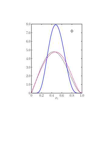
Figure 2: The distribution amplitudes (64) (dotted), (67) (solid) and the one corresponding to the wave function (68) (dashed line) versus $x_{1}$ at $x_{2}=x_{3}$. (colors online)

Ref.	$N$	$a$	$P$	$\langle k^{2}_{\perp}\rangle^{1/2}$	comment
	$[\,{\rm GeV}^{-2}]$	$[\,{\rm GeV}^{-1}]$		$[\,{\rm MeV}]$
BK (63)	160.5	0.75	0.17	417
(76)	61.8	1.1	0.5	280	diquark
KK (66), (67)	2117	0.75	0.90	460	$\rho=2.0$
BB (66), (68)	3477	0.75	0.90	431	$\rho=2.0$
(77)	169.5	1.1	0.90	317	diquark

Table 1: The parameters of the light-cone wave functions used for the calculation of the $u\to c$ transition GPDs. For the $\Lambda_{c}$ the quoted r.m.s. transverse momentum is that of the heavy quark.

According to the HQET [13] the major part of the $\Lambda_{c}$ state comes from the configuration where the $c$ quark carries the helicity of its parent baryon while the two light quarks are coupled in a spin-isospin-zero state. In the formal limit of $m_{c}\to\infty$ there should be no admixture from configurations where the helicity of the $c$ quark is opposite to that of the $\Lambda_{c}$. However, for a $c$-quark mass of $1.27\,\,{\rm GeV}$ which is large enough to justify the application of HQET ideas but too small in order to suppress corrections to the HQET decisively, a small admixture from a $c$-quark with helicity opposite to that of the $\Lambda_{c}$ cannot be excluded. We therefore write the valence Fock state of the $\Lambda_{c}$ in the form

$$\mid\Lambda_{c}^{+},+;cud\rangle\,=\,\int[dx]_{3}[d^{2}{\bf k}_{\perp}]_{3}\Big{\{}({\cal M}^{c}_{++-}-{\cal M}^{c}_{+-+})+\rho(x_{2}-x_{3}){\cal M}^{c}_{-++}\Big{\}}\,\Psi_{\Lambda}(x_{i},{\bf k}_{\perp}{}_{i})\,,$$ (65)

where ${\cal M}^{c}_{\lambda_{1}\lambda_{2}\lambda_{3}}$ are the three-quark states defined in (62) with the first $u$ quark being replaced by the $c$ quark. The scalar wave function, $\Psi_{\Lambda}$, must be symmetric under the interchange of the momentum fractions of the two light quarks. The factor $x_{2}-x_{3}$ in (65) takes care of the isospin of the $\rho$ term [36]. It also guarantees the vanishing of the $\rho$-term in the formal limit $m_{c}\to\infty$ as is required by the HQET.

We know from the LEP experiments [37, 38, 39] that the polarization of the $b$ quark generated in the process $e^{+}e^{-}\to Z\to b\bar{b}$ ($P_{b}=-0.94$) is not fully transferred to the $\Lambda_{b}$ baryon as is predicted by the HQET. Rather the $\Lambda_{b}$ polarization only amounts to $-0.43\pm 0.25$ as an average of the three experimental results. A substantial fraction of the observed $\Lambda_{b}$ baryons likely comes from the decay of the $\Sigma_{b}$ and $\Sigma^{*}_{b}$ which leads to a strong depolarization of the $\Lambda_{b}$. Whether this explains the observed $\Lambda_{b}$ polarization fully or only partially is unknown. Hence, the possibility that there is an admixture from configurations where the $\Lambda_{b}$ and the $b$ quark have opposite helicities cannot be ruled out at present. It is plausible to expect that for the lighter $c$-quark system this configuration is even more important. We therefore allow for it and take a value of 2.0 for the mixing parameter $\rho$. The configuration with opposite helicity then contributes about $10\%$ to the probability of the $\Lambda_{c}$ state (65).

We parameterize the scalar wave function in (65) as

$$\Psi_{\Lambda}\,=\,N_{\Lambda}\exp{\big{[}-f(x_{1})\big{]}}\exp{\Big{[}-a_{\Lambda}^{2}\sum\frac{{\bf k}_{\perp}{}_{i}^{2}}{x_{i}}\Big{]}}\,.$$ (66)

The function $f(x_{1})$ has to generate the expected pronounced peak at $x_{1}\simeq x_{0}$ as defined in (5). Current model wave functions for the $\Lambda_{c}$ possess this property [5, 16, 17, 40, 41, 42]. For $f(x_{1})$ we adopt a slightly modified version of the one given in [16],

$$f_{KK}(x_{1})\,=\,a_{\Lambda}^{2}M^{2}\frac{(x_{1}-x_{0})^{2}}{x_{1}(1-x_{1})}\,.$$ (67)

The LCWF (66) is a suitable adaptation of the one proposed in [41] which has been obtained by transforming a harmonic oscillator wave function to the light cone [42].

As an alternative we will also make use of a result from QCD sum rules obtained for the $\Lambda_{b}$ baryon [17] which we adapt to our case of a charm baryon, namely

$$f_{BB}(x_{1})\,=\,a_{\Lambda}M(1-x_{1})\,.$$ (68)

Up to corrections of order $(M-m_{c})/M$ the two functions have the same $x_{1}$ dependence for large $m_{c}$. The parameters of the two choices for the $\Lambda_{c}$ wave function are quoted in Tab. 1. We assume $a_{p}=a_{\Lambda}$ and a probability of $0.9$. The normalization $N_{\Lambda}$ is fixed from these parameters. A large value of the $\Lambda_{c}$ valence Fock state probability is to be expected [41].

The distribution amplitude corresponding to (66) reads

$$\Phi^{a}_{\Lambda}\propto x_{1}x_{2}x_{3}\exp{\big{[}-f(x_{1})\big{]}}\,.$$ (69)

The two $\Lambda_{c}$ distributions amplitudes are compared to each other and to the proton distribution amplitude in Fig. 2. The variant (68) is broader than (67) and is very similar to the proton distribution amplitude. Since the $c$ quark is relatively light the peak positions of the $\Lambda_{c}$ and the proton distribution amplitudes do not differ much. For the case of the $\Lambda_{b}$, for instance, the peak positions would differ markedly.

The GPDs are obtained from the following overlap integrals [26]

$$H^{cu}_{T}(\bar{x},\xi,t) = -\frac{1}{1-\xi^{2}}\int[d\bar{x}]_{3}[d^{\,2}{\bf k}_{\perp}]_{3}\delta(\bar{x}-\bar{x}_{1})\Psi_{\Lambda}(\hat{x}_{i},\hat{k}_{\perp i})$$

$$\times \Big{[}\Psi_{123}(\tilde{x}_{i},\tilde{k}_{\perp i})+\Psi_{132}(\tilde{x}_{i},\tilde{k}_{\perp i})+\Psi_{231}(\tilde{x}_{i},\tilde{k}_{\perp i})\Big{]}\,,$$

$$\Delta H^{cu}(\bar{x},\xi,t) = -\frac{\rho}{1-\xi^{2}}\int[d\bar{x}]_{3}[d^{\,2}{\bf k}_{\perp}]_{3}\delta(\bar{x}-\bar{x}_{1})\Psi_{\Lambda}(\hat{x}_{i},\hat{k}_{\perp i})$$ (70)

$$\times (\hat{x}_{2}-\hat{x}_{3})\Psi_{213}(\tilde{x}_{i},\tilde{k}_{\perp i})\,,$$

and the GPDs $H$ and $\widetilde{H}$ are given by the combinations

$$H^{cu}\,=\,H^{cu}_{T}-\Delta H^{cu}\,,\qquad\widetilde{H}^{cu}\,=\,H^{cu}_{T}+\Delta H^{cu}\,.$$ (71)

All other GPDs are zero. They require parton orbital angular momentum, a property that our simple wave functions for the $\Lambda_{c}$ do not possess. At least for large $m_{c}$ its structure follows from the HQET. The proton wave functions might have a more complicated structure involving, for instance, components with non-zero orbital angular momentum. This would still lead to the same result for the GPDs since the overlap with the $\Lambda_{c}$ LCWF does project out only $L=0$ components of the proton wave function.

The arguments of the light-cone wave functions are related to the average parton momenta, over which it is to be integrated, by [26]

$$\tilde{x}_{1} = \frac{\bar{x}_{1}+\xi}{1+\xi}\,,\qquad\tilde{k}_{\perp 1}\,=\,\bar{k}_{\perp 1}-\frac{1-\bar{x}_{1}}{1+\xi}\frac{{\bf\Delta}_{\perp}}{2}\,,$$

$$\tilde{x}_{j} = \frac{\bar{x}_{j}}{1+\xi}\,,\qquad\;\tilde{k}_{\perp j}\,=\,\bar{k}_{\perp j}+\frac{\bar{x}_{j}}{1+\xi}\frac{{\bf\Delta}_{\perp}}{2}\,,\quad{\rm for}\;\;j=2,3,$$

$$\hat{x}_{1} = \frac{\bar{x}_{1}-\xi}{1-\xi}\,,\qquad\hat{k}_{\perp 1}\,=\,\bar{k}_{\perp 1}+\frac{1-\bar{x}_{1}}{1-\xi}\frac{{\bf\Delta}_{\perp}}{2}\,,$$

$$\hat{x}_{j} = \frac{\bar{x}_{j}}{1-\xi}\,,\qquad\;\hat{k}_{\perp j}\,=\,\bar{k}_{\perp j}-\frac{\bar{x}_{j}}{1-\xi}\frac{{\bf\Delta}_{\perp}}{2}\,,\quad{\rm for}\;\;j=2,3.$$ (72)

Working out these integrals for the wave functions (63) and (66) we obtain the GPD $H^{cu}_{T}$

$$H^{cu}_{T} = -\frac{3}{4}\frac{N_{\Lambda}N_{p}}{(4\pi)^{4}}\frac{1}{1-\xi^{2}}\frac{\bar{x}^{2}-\xi^{2}}{a^{2}_{p}(1+\xi)+a^{2}_{\Lambda}(1-\xi)}$$ (73)

$$\times \frac{(1-\bar{x})^{3}}{1+\xi}\frac{1+2\xi+\bar{x}}{a_{p}^{2}(1+\xi)^{2}(\bar{x}-\xi)+a^{2}_{\Lambda}(1-\xi)^{2}(\bar{x}+\xi)}$$

$$\times \exp{\Big{[}-f\Big{(}\frac{\bar{x}-\xi}{1-\xi}\Big{)}\Big{]}}\,\exp{\Big{[}\frac{-(1-\bar{x})\,a^{2}_{\Lambda}a^{2}_{p}\,\Delta_{\perp}^{2}}{a_{p}^{2}(1+\xi)^{2}(\bar{x}-\xi)+a^{2}_{\Lambda}(1-\xi)^{2}(\bar{x}+\xi)}\Big{]}}\,,$$

and for the $\rho$-dependent part

$$\Delta H^{cu}\,=\,\frac{\rho}{15}\frac{1}{1-\xi}\,\frac{(1-\bar{x})^{2}}{1+2\xi+\bar{x}}\,H^{cu}_{T}\,.$$ (74)

The GPD $H_{T}$ is shown in Fig. 3. One observes that the GPD exhibits the anticipated pronounced peak at $\bar{x}\simeq x_{0}$. With increasing $\Delta_{\perp}^{2}$ (or $-t^{\prime}$, see Eq. (98)) the position of the peak is slightly shifted towards larger values of $\bar{x}$. This property of the $u\to c$ transition GPDs is similar to that of the proton valence-quark GPDs which have been determined from an analysis of the nucleon form factors through the familiar GPD sum rules in Ref. [18]. The only difference is that the $u\to c$ transition GPDs possess this property already at $t^{\prime}=0$ as a consequence of the intrinsic scale $4m_{c}^{2}$. The proton GPDs exhibit a peak only at large values of $-t$ and, therefore, the handbag approach can be applied to (real) Compton scattering only at wide angles. The two variants of the mass exponential entail striking differences in shape of the resulting GPDs displayed in Fig. 3. The GPD evaluated from (68) is much broader than the other one. The maxima of the GPD evaluated from (68) are sited at lower values of $\bar{x}$ for small $\Delta_{\perp}^{2}$ but at slightly larger ones for large $\Delta_{\perp}^{2}$ than is obtained from (67). The differences between the two GPDs have a bearing on the form factors and predicted cross sections as we are going to discuss in the following.

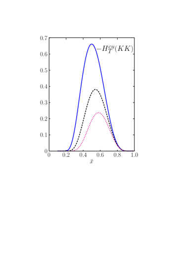
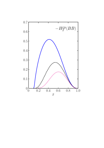
Figure 3: The $u\to c$ transition GPD $H_{T}$ obtained from the overlap of the LCWFs (63) and (66) (for the variants (67) (left) and (68) (right)) versus $\bar{x}$ at $s=30\,\,{\rm GeV}^{2}$ and $\Delta_{\perp}^{2}=0,2.0,4.0\,\,{\rm GeV}^{2}$, corresponding to $t^{\prime}=0,-2.17,-4.41\,\,{\rm GeV}^{2}$ ($\xi=0.112,0.123,0.139$) shown as solid, dashed and dotted lines, respectively (colors online).

With the GPDs at hand the transition form factors can be evaluated according to (41). They exhibit a structure analogously to (71)

$$R_{V}(\xi,t)\,=\,S_{T}(\xi,t)-\Delta R(\xi,t)\,,\quad R_{A}(\xi,t)\,=\,S_{T}(\xi,t)+\Delta R(\xi,t)\,.$$ (75)

In Fig. 4 the form factors $S_{T}$ and $\Delta R$, scaled by $t^{\prime}$ for the ease of graphical representation, are shown at $s=30\,\,{\rm GeV}^{2}$. The differences between the models (67) and (68) are particularly substantial at small $\Delta_{\perp}^{2}$ or $-t^{\prime}$. Also displayed in Fig. 4 is the approximation (42). As can be observed it is very close to the full form factor. This approximate coincidence nicely demonstrates the internal consistency of the peaking approximation. As the figure also reveals, $\Delta R$ is tiny despite the fact that the $\rho$ term in (65) contributes as much as $10\%$ to the probability of the $\Lambda_{c}^{+}$ state. The strong suppression of $\Delta R$ is a consequence of the tiny overlap of the $\rho$ term in the $\Lambda_{c}$ state with the proton wave function which manifests itself in the factor $(1-\bar{x})^{2}$ in (74). Even by a doubling of $\rho$, which leads to the implausibly large contribution of $30\%$ to the probability of the $\Lambda_{c}$ valence Fock state, we obtain $\mid\Delta R\mid\ll\mid S_{T}\mid$. Thus, $\Delta R$ is so small that it has no direct bearing on the observables for realistic values of $\rho$.

Let us now turn to the issue of the error assessment. It is true that the independent parameters of the $\Lambda_{c}$ LCWF are the normalization and the transverse size parameter, but we do not have any idea about their uncertainties in contrast to the probability and the r.m.s. transverse momentum. We, therefore, assume errors for the latter quantities and vary $N_{\Lambda}$ and $a_{\Lambda}$ as well as $m_{c}$ (within the PDG limits (6)) in such a way that the errors of $P_{\Lambda}$ and $\langle k^{2}_{\perp}\rangle^{1/2}$ are covered. For the latter quantity we assume an error of $\pm 10\%$ which is in fair agreement with an estimate of it for heavy baryons made in [40]. For the probability of the $\Lambda_{c}$ valence Fock state we allow for the maximum value of 1 and take as its lowest value 0.7. The described estimate of the parametric error is shown for the form factor $S_{T}$ in Fig. 4. We do not take into account the uncertainties of the proton wave function. They are small compared to that of the $\Lambda_{c}$ wave function since the proton wave function is determined from detailed fits to nucleon form factors and parton distributions [28]. The uncertainty of the form factor evaluated from the mass exponential (68) is of about the same size as for the variant (67).

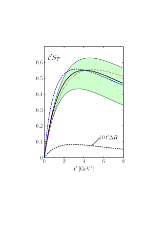
Figure 4: The transition form factor $S_{T}$ scaled by $t^{\prime}$ versus $t^{\prime}$ at $s=30\,{\rm GeV}^{2}$ evaluated from (73) using (67). The band indicates the parametric uncertainties of the form factor. The dashed line represents the the result obtained with (68) instead of (67) and the dotted line the approximation (42). The lower dashed line is 10 times the corresponding scaled form factor $\Delta R$ (colors online).

It is popular to model the baryons as a quark-diquark state. For the case of the $\Lambda_{c}$ this appears rather natural with regard to the HQET and indeed many examples of quark-diquark wave functions for the $\Lambda_{c}$ can be found in the literature [5, 16, 40, 43, 44, 45]. In all these cases only a spin-isospin scalar diquark, $S_{[ud]}$, is used, an assumption that is in accordance with the large-$m_{c}$ limit of the HQET. In view of our experience with the three-quark models we omit a possible admixture of other diquarks for simplicity. The proton may have a more complicated spectator structure with scalar and axial-vector diquarks and perhaps excitations of higher states involving angular momentum [46]. But as we mentioned in the discussion of the 3-quark models, the overlap with the $\Lambda_{c}^{+}$ LCWF only projects out the corresponding component with the scalar diquark from the proton LCWF. In order to render possible a comparison with the results presented in [5] we also employ the quark-diquark model here. For the ease of comparison we use the same parameters as in [5] although the LCWFs are slightly modified in order to take care of recent developments.

According to [5] we write the wave function of a proton in an $u_{\pm}S_{[ud]}$ Fock state as

$$\Psi_{p(qD)}\,=\,N_{p(qD)}(1-x)\exp{\big{[}-\frac{a_{p(qD)}^{2}{\bf k}_{\perp}^{2}}{x(1-x)}\big{]}}\,.$$ (76)

The parameters of this wave function are quoted in Tab. 1. The probability of 0.5 for a proton may appear rather large. However, one may argue that a diquark is a bound state of two quarks and embodies therefore also gluons and sea quarks. Hence, the quark-diquark wave function effectively takes into account higher Fock states and has therefore a larger probability than one would expect for a 3-quark valence-Fock-state wave function. In view of this fact a larger transverse size of the quark-diquark state appears plausible, too.

For the LCWF of a $\Lambda_{c}^{+}$ in a $c_{\pm}S_{[ud]}$ state we use

$$\Psi_{\Lambda(qD)}\,=\,N_{\Lambda(qD)}(1-x)\exp{\Big{[}-a_{\Lambda(qD)}^{2}M^{2}\frac{(x-x_{0})^{2}}{x(1-x)}\Big{]}}\exp{\Big{[}-\frac{a_{\Lambda(qD)}^{2}{\bf k}_{\perp}^{2}}{x(1-x)}\Big{]}}\,.$$ (77)

The parameters are again listed in Tab. 1.

The overlap of the two wave functions (76) and (77) provides the following result for $H=\widetilde{H}=H_{T}$

$$H^{cu}_{T} = \frac{N_{\Lambda(qD)}N_{p(qD)}}{16\pi^{2}}\frac{1}{(1-\xi^{2})^{3/2}}\frac{(1-\bar{x})^{3}(\bar{x}^{2}-\xi^{2})}{a_{\Lambda(qD)}^{2}(1-\xi)^{2}(\bar{x}+\xi)+a_{p(qD)}^{2}(1+\xi)^{2}(\bar{x}-\xi)}$$ (78)

$$\times \exp{\Big{[}-a_{\Lambda(qD)}^{2}M^{2}\frac{(\bar{x}-\xi-x_{0}(1-\xi))^{2}}{(\bar{x}-\xi)(1-\bar{x})}\Big{]}}$$

$$\times \exp{\Big{[}\frac{-(1-\bar{x})a_{\Lambda(qD)}^{2}a_{p(qD)}^{2}\,\Delta_{\perp}^{2}}{a_{\Lambda(qD)}^{2}(1-\xi)^{2}(\bar{x}+\xi)+a_{p(qD)}^{2}(1+\xi)^{2}(\bar{x}-\xi)}\Big{]}}\,.$$

The other GPDs are zero. The quark-diquark GPD has a similar shape as the 3-quark GPDs. Only its size is larger by about a factor of 1.6. The form factors $R_{V}=R_{A}=S_{T}$ in the quark-diquark model also behave similar to those in the 3-quark model.

5 Observables

5.1 Cross sections

The differential cross section for the process $p\bar{p}\to\Lambda_{c}^{+}\bar{\Lambda}_{c}^{-}$ reads

$$\frac{d\sigma}{d\Omega}\,=\,\frac{1}{4\pi}s\Lambda_{m}\Lambda_{M}\frac{d\sigma}{dt}\,=\,\frac{1}{64\pi^{2}}\,\frac{1}{s}\frac{\Lambda_{M}}{\Lambda_{m}}\sigma_{0}\,,$$ (79)

where

$$\sigma_{0}\,=\,\frac{1}{4}\sum\left|{\cal M}_{\mu^{\prime}\nu^{\prime},\mu\nu}\right|^{2}\,.$$ (80)

The cross section can readily be calculated from the amplitudes (55) using the subprocess amplitudes given in (48) and appropriate form factors. Particularly simple are those GPD models in which the $\Lambda_{c}$ only consists of the configuration where the two light quarks are coupled in a spin-isospin-zero state (bound in a diquark or not) as is predicted by the HQET. They do not involve quark orbital angular momentum and the parameter $\rho$ is zero. As we discussed in the preceding section a non-zero value of $\rho$ is possible but cannot be large as estimated from measurements of the $\Lambda_{b}$ polarization at LEP [37, 38, 39]. In the cases we examine, the $\rho$ term does only lead to tiny differences in the form factors. Practically, there is only one independent form factor

$$S_{T}(\xi,t)\simeq R_{V}(\xi,t)\simeq R_{A}(\xi,t)\,.$$ (81)

All other form factors are zero. In a situation where (81) holds, the differential cross section strongly simplifies and becomes proportional to the subprocess one

$$\frac{d\sigma}{d\Omega}(p\bar{p}\to\Lambda_{c}^{+}\bar{\Lambda}_{c}^{-})\,=\,\left(\frac{C_{F}}{N_{C}}\right)^{2}(1-\xi^{2})^{2}\Big{(}\frac{m_{c}}{M}\Big{)}^{2}\frac{S_{T}^{\,4}(\xi,t)}{\Lambda_{m}}\;\frac{d\hat{\sigma}}{d\hat{\Omega}}({u}\bar{u}\to{c}\bar{c})\,.$$ (82)

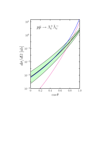
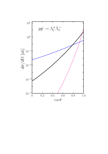
Figure 5: Predictions for the differential cross section versus $\cos{\theta}$. Left: $s=30\,\,{\rm GeV}^{2}$. Solid line represents the result evaluated from (73) with the mass exponential (67) (with error band). The dashed line is obtained with (68) and the dotted one is the results from the quark-diquark model. Right: The differential cross section at $s=23\,,30$ and $50\,\,{\rm GeV}^{2}$ shown as dashed, solid and dotted line, respectively. The cross sections are evaluated from (73) with the mass exponential (67) (colors online).

Results for the differential cross sections are shown in Fig. 5. The differential cross section is sharply forward peaked. This effect becomes more pronounced for higher energies. It arises from the dominance of the amplitude ${\cal M}_{+-,+-}$ ($\propto\cos^{2}{\theta/2}$) near the forward direction and is natural given that we consider an annihilation reaction at high energies. The effect is pronounced by the behavior of the form factors which obey (81) and decrease monotonically with increasing $-t^{\prime}$. The cross section increases with $s$ for small scattering angles near the forward direction. This is a transient effect which disappears at large $s$ and $d\sigma/d\Omega$ ultimately show the usual $1/s$ decrease since the form factors become independent on $\xi$ in that region as we mentioned in Sect. 2.3. The various models we employ behave similar in that respect. The quark-diquark model predicts a particularly steeply falling cross section. This feature is only to be expected given the small values of the r.m.s. transverse momenta in that model or the associated large transverse sizes (see Tab.  1). It can also be seen in Fig. 5 that the use of the mass exponential (68) instead of (67) provides markedly larger differential cross sections for small-angle scattering.

The integrated cross section is displayed in Fig. 6. Its magnitude is of order nb. As the behavior of the differential cross section indicates (see Fig. 5) the largest cross section is obtained with the mass exponential (68). For comparison we note that in [5] the $p\bar{p}\to\Lambda_{c}^{+}\bar{\Lambda}_{c}^{-}$ cross section was estimated to amount to about 3(10) nb at $s=30(50)\,\,{\rm GeV}^{2}$. This is in reasonable agreement with the predictions from the quark-diquark model as well as the other ones presented here.

In Sect. 4 we have already discussed the model uncertainties of the form factors. These uncertainties enter directly into the errors of the cross section (note that it is related to the fourth power of the form factor). The errors are shown as bands in Figs. 5 and 6. The width of the bands correspond to a probability of the relevant $\rho$-independent term in the $\Lambda_{c}$ state (65) varying between 0.9 and 0.6 and to an error of $\pm 10\%$ for the r.m.s. charm-quark transverse momentum. All the models we exploit have similar parametric errors. Larger than these parametric errors is the difference between the predictions obtained from the different mass exponentials which is rather representative for the uncertainties of our predictions.

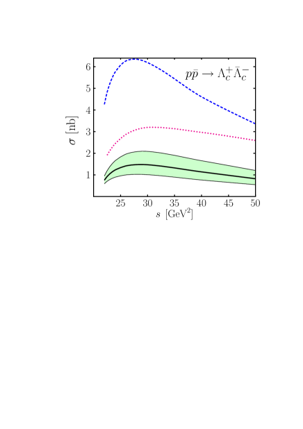
Figure 6: The integrated cross section ($\cos\theta\geq 0$) versus $s$. For notation we refer to the left hand side of Fig. 5.

5.2 Spin dependence

For spin-dependent observables we have to take care of the fact that experiments provide typically c.m.s. observables which are expressed in terms of c.m.s. helicity amplitudes ($\Phi$). We therefore have to transform our light-cone amplitudes (53), (55) to the c.m.s. ones (57) with the help of the parameter $\beta$ given in (58). We note that for observables that only refer to the helicities of the initial state baryons this transform has no effect up to corrections of order $m/\sqrt{s}$. We also remark that the unpolarized cross section can be worked out in either basis, it is independent on the transform (57).

While all single-spin asymmetries are zero to lowest order of perturbative QCD, there are many non-zero spin correlation parameter in our approach. We employ the conventions for the notation of such observables advocated for in [47]. The directions of the spin of the particles are denoted by $L\dots$ helicity, $N\dots$ normal to scattering plane, $S\dots$ ‘sideways’ spin direction within scattering plane but orthogonal to direction of momentum,

$${\bf L}_{i}\,=\,{\bf p}_{i}/{p_{i}}\,,\qquad{\bf N}\,=\,{\bf L}_{p}\times{\bf L}^{\prime}_{\Lambda}\,,\qquad{\bf S}_{i}\,=\,{\bf N}\times{\bf L}_{i}\,.$$ (83)

The corresponding spin states for $N$ and $S$ type polarizations read

$$\mid\uparrow(\downarrow)\rangle\,=\,\frac{1}{\sqrt{2}}\,\Big{[}\mid+\rangle+(-)\imath\mid-\rangle\Big{]}\,,\qquad\mid\to(\leftarrow)\rangle\,=\,\frac{1}{\sqrt{2}}\,\Big{[}\mid+\rangle+(-)\mid-\rangle\Big{]}\,,$$ (84)

respectively. The spin-spin correlation parameters are denoted by ($i,j=L,N,S$):
               initial state spin correlations                                  $\quad-\quad A_{ij}$,
               final state spin correlations                                     $\quad-\quad C_{ij}$,
               polarization transfer from $p(\overline{p})$ to $\Lambda_{c}^{+}(\overline{\Lambda}{}_{c}^{-})$              $\quad-\quad D_{ij}(\overline{D}_{ij})$,
               polarization correlation between $p(\overline{p})$ and $\overline{\Lambda}{}_{c}^{-}(\Lambda_{c}^{+})$ $\quad-\quad K_{ij}(\overline{K}_{ij})$.

A spin correlation parameter is defined by

$${\cal O}_{ij}\,=\,\frac{\sigma(ij)+\sigma(-i-j)-\sigma(i-j)-\sigma(-ij)}{\sigma(ij)+\sigma(-i-j)+\sigma(i-j)+\sigma(-ij)}\,,$$ (85)

where $\sigma(ij)$ stands for the differential cross section for the scattering with two particles in given spin states. For all GPD models that approximately possess the property (81), the spin correlations simply read 

$${\cal O}(p\bar{p}\to\Lambda_{c}^{+}\bar{\Lambda}_{c}^{+})\,=\,{\cal O}({u}\bar{u}\to{c}\bar{c})\,.$$ (86)

The form factors and, hence, their uncertainties, cancel out in the spin correlations. Thus, all our GPD models lead to the same set of predictions for these observables. In this sense our predictions for spin correlations are model independent.

Below we list a set of examples of spin correlations obtained in the handbag approach from form factors which satisfy the relation (81). If the parameter $\beta$ is only taken into account up to linear order, which is justified for not too large scattering angles, the corresponding analytical expressions become rather simple:

$$A_{LL} = -1\,,$$

$$C_{LL} = -\frac{1+\cos^{2}{\theta}-4M^{2}/s\sin^{2}{\theta}+8\beta M/\sqrt{s}\sin{2\theta}}{1+\cos^{2}{\theta}+4M^{2}/s\sin^{2}{\theta}}\,,$$

$$D_{LL} = -K_{LL}\,=\,2\frac{\cos{\theta}+4\beta M/\sqrt{s}\sin{\theta}}{1+\cos^{2}{\theta}+4M^{2}/s\sin^{2}{\theta}}\,,$$

$$D_{NN} = D_{SS}\,=\,0\,,$$

$$A_{NN} = C_{NN}\,=\,-\sin^{2}{\theta}\,\frac{1-4M^{2}/s}{1+\cos^{2}{\theta}+4M^{2}/s\sin^{2}{\theta}}\,,$$

$$C_{SS} = -\sin{\theta}\,\frac{\sin{\theta}(1+4M^{2}/s)-16\beta M/\sqrt{s}\cos{\theta}}{1+\cos^{2}{\theta}+4M^{2}/s\sin^{2}{\theta}}\,,$$

$$C_{LS} = -4\frac{M/\sqrt{s}\sin{\theta}\cos{\theta}-\beta\cos^{2}{\theta}+4\beta M^{2}/s\sin^{2}{\theta}}{1+\cos^{2}{\theta}+4M^{2}/s\sin^{2}{\theta}}\,,$$

$$C_{LN} = C_{NS}\,=\,0\,.$$ (87)

As for single spin asymmetries (cf. the remark in Sect. 3.1) the observables $D_{NN}$, $C_{NS}$ and $C_{LN}$ are related to the imaginary parts of interference terms and are therefore zero to lowest order of perturbative QCD. To higher orders they may be non-zero. In Fig. 7 we show results for some of the spin correlations. Since these predictions extend to c.m.s. scattering angles up to $90^{\circ}$ the $\beta$ dependence of the spin correlations has been fully taken into account (beyond linear order) in the numerical evaluation.

Figure 7: Final state helicity correlations $C_{ij}$ and the $p\to\Lambda_{c}$ polarization transfer $D_{LL}$ versus $\cos{\theta}$ at $s=30\,\,{\rm GeV}^{2}$. (colors online)

6 Summary

We have analyzed the exclusive production of $\Lambda_{c}^{+}\bar{\Lambda}{}_{c}^{-}$ pairs in proton-antiproton collisions. We have argued that this process is mediated by collinear emission of soft $u$ ($\bar{u}$) quarks from the (anti-)proton, a hard scattering $u\bar{u}\to c\bar{c}$ and subsequently a collinear absorption of $c$ ($\bar{c}$) quarks by the remainders of the (anti-)proton turning them into the final $\Lambda_{c}^{+}$ ($\bar{\Lambda}_{c}^{-}$). The hard subprocess is calculable within perturbative QCD to a given order. As we showed the hadronic matrix elements that describe the $p\to\Lambda_{c}^{+}$ ($\bar{p}\to\bar{\Lambda}_{c}^{-}$) transition, can be parameterized in terms of GPDs. The process amplitudes thus factorize into a product of hard subprocess amplitudes and $1/\bar{x}$ moments of GPDs, i.e. generalized form factors as, for instance, in wide-angle Compton scattering.

To model the GPDs we employ the representation of the GPDs as overlaps of LCWFs for the involved baryons. The LCWFs for the valence Fock states of the baryons are taken from the literature. Although, in general, the restriction to the valence Fock states is insufficient for modelling the GPDs as a function of three variables $\bar{x}$, $\xi$ and $t$, it is expected to be a reasonable approximation for our case. As is predicted by the HQET, the $\Lambda_{c}$ valence Fock state is dominated by the simple configuration where the $c$ quark carries the helicity of the $\Lambda_{c}$ while the light quarks are coupled in a spin and isospin zero state with only little admixture of other configurations. It is also expected that higher Fock states play only a minor role for the $\Lambda_{c}$. A possible more complicated structure of the proton involving, for instance, parton orbital angular momentum or higher Fock states, is irrelevant since its overlap with the simple $\Lambda_{c}$ LCWF is zero. We therefore achieve rather robust model GPDs with only a few parameters, like the transverse size parameters or the normalizations of the LCWFs which can be adjusted within certain ranges without loosing their physical interpretation. With the GPDs at hand we are in the position to evaluate the form factors and, subsequently, to predict differential and integrated cross section as well as a number of spin correlation parameters. We emphasize that the prediction of the integrated cross section achieved here does not differ much from a previous estimate in a model that bears resemblance with the handbag approach [5].

We also note that the $u\to c$ transition GPDs do not only form the soft physics input for the handbag contribution to the process $p\bar{p}\to\Lambda_{c}^{+}\bar{\Lambda}{}_{c}^{-}$ but allows also to calculate the $\Lambda_{c}^{+}\to p$ transition form factors. Another possible application is electroproduction of charmed mesons (e.g. $ep\to e^{\prime}D(D^{*})\Lambda_{c}^{+}$). Extensions to other charmed baryons and to calculation of $\alpha_{s}$ corrections to the subprocess is left to a forthcoming paper.

Appendix A Kinematics

The momenta and light-cone helicities of the incoming proton and antiproton are denoted by $p$, $\mu$ and $q$, $\nu$, those of the outgoing $\Lambda_{c}^{+}$ and $\bar{\Lambda}{}_{c}^{-}$ by $p^{\prime}$, $\mu^{\prime}$, and $q^{\prime}$, $\nu^{\prime}$, respectively. The mass of the proton is denoted by $m$ that of the $\Lambda_{c}^{+}$ by $M$. We work in a center of mass frame where the baryon’s momenta in light-cone coordinates are parameterized as

$$p = \left[(1+\xi)\bar{p}^{+},\,\frac{m^{2}+\Delta_{\perp}^{2}/4}{2(1+\xi)\bar{p}^{+}},\,-\frac{{\bf\Delta}_{\perp}}{2}\right],\,p^{\prime}=\left[(1-\xi)\bar{p}^{+},\,\frac{M^{2}+\Delta_{\perp}^{2}/4}{2\bar{p}^{+}(1-\xi)},\,\phantom{-}\frac{{\bf\Delta}_{\perp}}{2}\right],$$

$$q = \left[\frac{m^{2}+\Delta_{\perp}^{2}/4}{2(1+\xi)\bar{p}^{+}},\,(1+\xi)\bar{p}^{+},\,\phantom{-}\frac{{\bf\Delta}_{\perp}}{2}\right],\,q^{\prime}=\left[\frac{M^{2}+\Delta_{\perp}^{2}/4}{2\bar{p}^{+}(1-\xi)},\,(1-\xi)\bar{p}^{+},\,-\frac{{\bf\Delta}_{\perp}}{2}\right].$$ (88)

It is convenient to introduce sum and differences of the baryon momenta

$$P\,=\,2\bar{p}\,=\,p+p^{\prime}\,,\qquad Q\,=\,q+q^{\prime}\,,\qquad\Delta=p^{\prime}-p=q-q^{\prime}\,.$$ (89)

The momentum transfer $\Delta$ is expressed by

$$\Delta\,=\,\Big{[}-2\xi\bar{p}^{+}\,,\frac{M^{2}(1+\xi)-m^{2}(1-\xi)+\xi\Delta_{\perp}^{2}/2}{2\bar{p}^{+}(1-\xi^{2})}\,,{\bf\Delta}_{\perp}\Big{]}\,.$$ (90)

The three-components of the c.m.s. momenta of the incoming (anti) proton, $(-)p_{3}$, and the outgoing (anti) $\Lambda_{c}$, $(-)p^{\prime}_{3}$, read

$$p_{3}\,=\,\frac{1}{2}\sqrt{s}\sqrt{\Lambda_{m}^{2}-\Delta_{\perp}^{2}/s}\,,\quad\mid p^{\prime}_{3}\mid\,=\,\frac{1}{2}\sqrt{s}\sqrt{\Lambda_{M}^{2}-\Delta_{\perp}^{2}/s}\,,$$ (91)

where $s=(p+q)^{2}=(p^{\prime}+q^{\prime})^{2}$ is the usual Mandelstam energy variable. We also introduce the abbreviation

$$\Lambda_{i}\,=\,\sqrt{1-4m_{i}^{2}/s}$$ (92)

in a more generic notation ($m_{i}$ stands for $m$, $M$, or the charm-quark mass $m_{c}$; for $m_{i}=m_{c}$ Mandelstam $s$ has to be replaced by $\hat{s}$). While the three-component of the incoming proton’s momentum is always positive that of the outgoing $\Lambda_{c}$ can become negative for large c.m.s. scattering angles because of the unequal-mass kinematics. This change of signs occurs at

$$\Delta_{\perp}^{2}{}_{\rm max}\,=\,s\Lambda^{2}_{M}\,.$$ (93)

Thus, due to the unequal-mass kinematics, $\Delta_{\perp}^{2}$ is zero for forward scattering, reaches the maximal value and decreases again towards zero for backward scattering. Skewness, defined as a ratio of light-cone plus-components of baryon momenta, $\xi=(p^{+}-p^{\prime+})/(p^{+}+p^{\prime+})$, can be expressed as

$$\xi = \frac{\sqrt{\Lambda_{m}^{2}-\Delta_{\perp}^{2}/s}-{\rm sign}(p^{\prime}_{3})\sqrt{\Lambda_{M}^{2}-\Delta_{\perp}^{2}/s}}{2+\sqrt{\Lambda_{m}^{2}-\Delta_{\perp}^{2}/s}+{\rm sign}(p^{\prime}_{3})\sqrt{\Lambda_{M}^{2}-\Delta_{\perp}^{2}/s}}$$ (94)

$$= \frac{\Lambda_{m}^{2}-\Lambda_{M}^{2}}{\sqrt{\Lambda_{m}^{2}+\Lambda_{M}^{2}+2\Lambda_{m}\Lambda_{M}\cos\theta}}\,\frac{1}{2+\sqrt{\Lambda_{m}^{2}+\Lambda_{M}^{2}+2\Lambda_{m}\Lambda_{M}\cos\theta}}$$

$$\to \frac{M^{2}-m^{2}}{2s}\,\Big{[}1+\frac{3}{2}\frac{M^{2}+m^{2}+\Delta_{\perp}^{2}/2}{s}\Big{]}\quad{\rm for\;}s\to\infty\,,$$

where $\theta$ is the c.m.s. scattering angle. In a similar fashion can the other parameter occurring in the definition of the baryon momenta (88) be written as

$$\bar{p}^{+} = \frac{1}{4}\sqrt{\frac{s}{2}}\Big{[}2+\sqrt{\Lambda_{m}^{2}-\Delta_{\perp}^{2}/s}+{\rm sign}(p^{\prime}_{3})\sqrt{\Lambda_{M}^{2}-\Delta_{\perp}^{2}/s}\Big{]}$$ (95)

$$= \frac{1}{4}\sqrt{\frac{s}{2}}\Big{[}2+\sqrt{\Lambda_{m}^{2}+\Lambda_{M}^{2}+2\Lambda_{m}\Lambda_{M}\cos\theta}\Big{]}\,.$$

As a consequence of the unequal mass kinematics $\xi$ cannot become zero. For $p^{\prime}_{3}\geq 0$, however, the skewness is fairly small and tends to zero for $s\to\infty$.

The squared invariant momentum transfer is given by

$$t = \Delta^{2}\,=\,-\frac{\Delta_{\perp}^{2}}{1-\xi^{2}}-\frac{2\xi}{1-\xi^{2}}\Big{[}(1+\xi)M^{2}-(1-\xi)m^{2}\Big{]}$$ (96)

$$= -\frac{\Delta_{\perp}^{2}}{2}-\frac{s}{4}\Big{[}\Lambda_{m}^{2}+\Lambda_{M}^{2}-2{\rm sign}(p^{\prime}_{3})\sqrt{\Lambda_{m}^{2}-\Delta_{\perp}^{2}/s}\sqrt{\Lambda_{M}^{2}-\Delta_{\perp}^{2}/s}\Big{]}$$

$$= -\frac{s}{4}\Big{[}\Lambda_{m}^{2}+\Lambda_{M}^{2}-2\Lambda_{m}\Lambda_{M}\cos\theta\Big{]}\,.$$

It cannot become zero for forward scattering but acquires the value ($\xi_{0}=\xi(\Delta_{\perp}^{2}=0,p^{\prime}_{3}\geq 0)$):

$$t_{0}\,=\,t(\Delta_{\perp}^{2}=0,p^{\prime}_{3}\geq 0) = -\frac{2\xi_{0}}{1-\xi_{0}^{2}}\Big{[}(1+\xi_{0})M^{2}-(1-\xi_{0})m^{2}\Big{]}$$ (97)

$$= -\frac{s}{4}\,(\Lambda_{m}-\Lambda_{M})^{2}\,.$$

It is convenient to introduce a variable $t^{\prime}$ that vanishes for forward scattering. It is defined by

$$t^{\prime} = t-t_{0}\,=\,-\frac{\Delta_{\perp}^{2}}{2}-\frac{s}{2}\Big{[}\Lambda_{m}\Lambda_{M}-{\rm sign}(p^{\prime}_{3})\sqrt{\Lambda_{m}^{2}-\Delta_{\perp}^{2}/s}\sqrt{\Lambda_{M}^{2}-\Delta_{\perp}^{2}/s}\Big{]}$$ (98)

$$= -\frac{s}{2}\Lambda_{m}\Lambda_{M}\Big{[}1-\cos\theta\Big{]}\,.$$

Solving (98) for $\Delta_{\perp}^{2}$, one finds

$$\Delta_{\perp}^{2}\,=\,-t^{\prime}\frac{s\Lambda_{m}\Lambda_{M}+t^{\prime}}{s/4(\Lambda_{m}+\Lambda_{M})^{2}+t^{\prime}}\,=\,s\frac{\Lambda_{m}^{2}\Lambda_{M}^{2}\sin^{2}\theta}{\Lambda_{m}^{2}+\Lambda_{M}^{2}+2\Lambda_{m}\Lambda_{M}\cos\theta}\,.$$ (99)

Sine and cosine of half the c.m.s. scattering angle $\theta$ are connected with the Mandelstam variables by

$$\sin^{2}{\theta/2} = \frac{1-\cos{\theta}}{2}\,=\,\frac{t_{0}-t}{s\Lambda_{m}\Lambda_{M}}\,,$$

$$\cos^{2}{\theta/2} = \frac{1+\cos{\theta}}{2}\,=\,\frac{u_{1}-u}{s\Lambda_{m}\Lambda_{M}}\,,$$ (100)

where

$$u_{1}\,=\,u(\Delta_{\perp}^{2}=0,p^{\prime}_{3}\leq 0)\,=\,-\frac{s}{4}\,(\Lambda_{m}-\Lambda_{M})^{2}\,.$$ (101)

For forward scattering $u$ reads

$$u_{0}\,=\,u(\Delta_{\perp}^{2}=0,p^{\prime}_{3}\geq 0)\,=\,-\frac{s}{4}\,(\Lambda_{m}+\Lambda_{M})^{2}\,.$$ (102)

Appendix B The $u\to c$ generalized parton distributions

The vector current of bilocal quark field operators is defined as

$$V^{\mu}(-z^{-}/2,z^{-}/2)\,=\,\bar{\Psi}^{c}(-z^{-}/2)\gamma^{\mu}\Psi^{u}(z^{-}/2)-\bar{\Psi}^{u}(z^{-}/2)\gamma^{\mu}\Psi^{c}(-z^{-}/2)\,.$$ (103)

The Fourier transform of the plus component of its transition matrix element

$${\cal H}_{\mu^{\prime}\mu}^{\,cu}\,=\,\bar{p}^{+}\int\frac{dz^{-}}{2\pi}e^{\imath\bar{x}\bar{p}^{+}z^{-}}\langle\Lambda_{c}^{+};p^{\prime}\mu^{\prime}\mid V^{+}(-z^{-}/2,z^{-}/2)\mid p;p\mu\rangle\,,$$ (104)

can be decomposed into five covariant structures

$$\frac{P^{+}}{M+m}\bar{u}(p^{\prime})u(p)\,,\quad\frac{\Delta^{+}}{M+m}\bar{u}(p^{\prime})u(p)\,,\quad\bar{u}(p^{\prime})\gamma^{+}u(p)\,,$$

$$\bar{u}(p^{\prime})\frac{\imath\sigma^{+\nu}\Delta_{\nu}}{M+m}u(p)\,,\quad\bar{u}(p^{\prime})\frac{\imath\sigma^{+\nu}P_{\nu}}{M+m}u(p)\,.$$ (105)

The combinations of momenta are defined in (89). Helicity labels are omitted wherever it can be done without loss legibility. Only two of the covariant structures are independent since we have the familiar Gordon decomposition and analogous relations at disposal

$$P^{\mu}\bar{u}(p^{\prime})u(p) = (M+m)\bar{u}(p^{\prime})\gamma^{\mu}u(p)-\imath\bar{u}(p^{\prime})\sigma^{\mu\nu}\Delta_{\nu}u(p)\,,$$

$$\Delta^{\mu}\bar{u}(p^{\prime})u(p) = (M-m)\bar{u}(p^{\prime})\gamma^{\mu}u(p)-\imath\bar{u}(p^{\prime})\sigma^{\mu\nu}P_{\nu}u(p)\,.$$ (106)

In addition we have for the light-cone projections the relation

$$\Delta^{+}\,=\,-\xi P^{+}\,,$$ (107)

see (88) and (89). The two independent GPDs are chosen in analogy to the flavor-diagonal case (cf. [48])

$${\cal H}^{\,cu}_{\mu^{\prime}\mu}\,=\,\bar{u}(p^{\prime},\mu^{\prime})\left[H^{cu}(\bar{x},\xi,t)\,\gamma^{+}+E^{cu}(\bar{x},\xi,t)\,\frac{\imath\sigma^{+\nu}\Delta_{\nu}}{M+m}\right]u(p,\mu)\,.$$ (108)

In the unequal mass-case the matrix elements of the local vector current describing the electroweak $p\to\Lambda_{c}^{+}$ transition can be decomposed into three covariant structures for which one may choose

$$\langle\Lambda_{c}^{+};p^{\prime}\mu^{\prime}\mid V^{\mu}(0,0)\mid p;p\mu\rangle\,=\,\bar{u}(p^{\prime},\mu^{\prime})\Big{[}F_{V}\gamma^{\mu}\;+\;F_{T}\frac{\imath\sigma^{\mu\nu}\Delta_{\nu}}{m+M}\;+\;F_{3}\frac{\Delta^{\mu}}{M+m}\Big{]}u(p,\mu)\,.$$ (109)

The four-vectors $\Delta^{\mu}$ and $P^{\mu}$ are independent; only their plus components are proportional to each other.

Let us integrate (104) and (108) with respect to $\bar{x}$, which reduces the bilocal matrix element to a local one that describes the weak transition form factors for which we insert the form factor decomposition (109)

$$\int_{-1}^{1}d\bar{x}{\cal H}^{\,cu}_{\mu^{\prime}\mu} = \langle\Lambda_{c}^{+};p^{\prime}\mu^{\prime}\mid V^{+}(0,0)\mid p;p\mu\rangle$$ (110)

$$=\int_{-1}^{1}d\bar{x}H^{cu}(\bar{x},\xi,t)\,\bar{u}(p^{\prime},\mu^{\prime})\gamma^{+}u(p,\mu)+\int_{-1}^{1}d\bar{x}E^{cu}(\bar{x},\xi,t)\,\bar{u}(p^{\prime},\mu^{\prime})\frac{\imath\sigma^{+\nu}\Delta_{\nu}}{M+m}u(p,\mu)$$

$$=\bar{u}(p^{\prime},\mu^{\prime})\left[F_{V}(t)\,\gamma^{+}\;+\;F_{T}(t)\,\frac{\imath\sigma^{+\nu}\Delta_{\nu}}{m+M}\;+\;F_{3}(t)\,\frac{\Delta^{+}}{M+m}\right]u(p,\mu)\,.$$

Using again the Gordon decomposition (106) for the term $\propto F_{3}$, we find the following sum rules

$$\int_{-1}^{1}d\bar{x}H^{cu}(\bar{x},\xi,t) = F_{V}(t)-\xi F_{3}(t)\,,$$

$$\int_{-1}^{1}d\bar{x}E^{cu}(\bar{x},\xi,t) = F_{T}(t)+\xi F_{3}(t)\,.$$ (111)

In the limit of equal hadron masses conservation of the vector current requires $F_{3}=0$. To lowest order of the electroweak theory the weak transition form factors are zero; this holds in particular at the scale of $M_{Z}$. For lower scales, like $M$, there are effective operators that mediate $u\to c$ transitions through finite Wilson coefficients.

The lower vertex is treated analogously. It is related to the upper one by charge conjugation. It is then easy to show that

$$\langle\Lambda_{c}^{+}\mid V^{+}(-z/2,z/2)\mid p\rangle\,=\,-\langle\bar{\Lambda}_{c}^{-}\mid V^{+}(-z/2,z/2)\mid\bar{p}\rangle\,.$$ (112)

Taking the Fourier transform of this matrix element in analogy to (104), making the replacements

$$p\to q\,,\quad p^{\prime}\to q^{\prime}\,,\quad\Delta\to-\Delta\,,\quad\gamma^{+}\to\gamma^{-}\,,$$ (113)

and rewriting the right-hand side of (108) with the help of the behavior of the Dirac spinors under charge conjugation one finds for the lower vertex

$${\cal H}^{\,\overline{cu}}_{\nu^{\prime}\nu} = \bar{q}^{-}\int\frac{dz^{+}}{2\pi}e^{\imath\bar{x}\bar{q}^{-}z^{+}}\langle\bar{\Lambda}_{c}^{-};q^{\prime}\nu^{\prime}\mid V^{-}(-z^{+}/2,z^{+}/2)\mid\bar{p};q\nu\rangle$$ (114)

$$= \bar{v}(q,\nu)\left[H^{cu}(\bar{x},\xi,t)\,\gamma^{-}-E^{cu}(\bar{x},\xi,t)\,\frac{\imath\sigma^{-\nu}\Delta_{\nu}}{M+m}\right]v(q^{\prime},\nu^{\prime})\,.$$

The lowest moment of ${\cal H}_{\nu^{\prime}\nu}^{\overline{cu}}$ leads to the vector-current matrix element

$$\int_{-1}^{1}d\bar{x}{\cal H}^{\,\overline{cu}}_{\nu^{\prime}\nu} = \langle\bar{\Lambda}_{c}^{-};q^{\prime}\nu^{\prime}\mid V^{-}(0,0)\mid\bar{p};q\nu\rangle$$ (115)

$$=\int_{-1}^{1}d\bar{x}H^{cu}(\bar{x},\xi,t)\,\bar{v}(q,\nu)\gamma^{-}v(q^{\prime},\nu^{\prime})-\int_{-1}^{1}d\bar{x}E^{cu}(\bar{x},\xi,t)\,\bar{v}(q,\nu)\frac{\imath\sigma^{-\nu}\Delta_{\nu}}{M+m}v(q^{\prime},\nu^{\prime})$$

$$=\bar{v}(q,\nu)\,\left[F_{V}(t)\,\gamma^{-}-\;F_{T}(t)\,\frac{\imath\sigma^{-\nu}\Delta_{\nu}}{m+M}\;-\;F_{3}(t)\,\frac{\Delta^{-}}{M+m}\right]\,v(q^{\prime},\nu^{\prime})\,.$$

Using

$$\Delta^{-}\,=\,\xi Q^{-}\,,$$ (116)

and the Gordon decomposition

$$Q^{\mu}\bar{v}(q)v(q^{\prime})\,=\,-(M+m)\bar{v}(q)\gamma^{\mu}v(q^{\prime})-\imath\bar{v}(q)\sigma^{\mu\nu}\Delta_{\nu}v(q^{\prime})\,,$$ (117)

we find exactly the same sum rules as in (111).

Next we proceed analogously for the axial vector transition matrix element:

$$A^{\mu}(-z^{-}/2,z^{-}/2)\,=\,\bar{\Psi}^{c}(-z^{-}/2)\gamma^{\mu}\gamma_{5}\Psi^{u}(z^{-}/2)-\bar{\Psi}^{u}(z^{-}/2)\gamma^{\mu}\gamma_{5}\Psi^{c}(-z^{-}/2)\,,$$ (118)

$$\widetilde{\cal H}_{\mu^{\prime}\mu}^{\,cu}\,=\,\bar{p}^{+}\int\frac{dz^{-}}{2\pi}\,e^{\imath\bar{x}\bar{p}^{+}z^{-}}\langle\Lambda_{c}^{+};p^{\prime}\mu^{\prime}\mid A^{+}(-z^{-}/2,z^{-}/2)\mid p;p\mu\rangle\,,$$ (119)

can again be decomposed into five covariant structures

$$\frac{P^{+}}{M+m}\bar{u}(p^{\prime})\gamma_{5}u\,,\quad\frac{\Delta^{+}}{M+m}\bar{u}(p^{\prime})\gamma_{5}u\,,\quad\bar{u}(p^{\prime})\gamma^{+}\gamma_{5}u\,,$$

$$\bar{u}(p^{\prime})\frac{\imath\sigma^{+\nu}\Delta_{\nu}\gamma_{5}}{M+m}u\,,\quad\bar{u}(p^{\prime})\frac{\imath\sigma^{+\nu}P_{\nu}\gamma_{5}}{M+m}u\,.$$ (120)

We also have the two relations

$$\bar{u}(p^{\prime})\imath\sigma^{\mu\nu}P_{\nu}\gamma_{5}u(p) = (M+m)\bar{u}(p^{\prime})\gamma^{\mu}\gamma_{5}u(p)-\Delta^{\mu}\bar{u}(p^{\prime})\gamma_{5}u(p)\,,$$

$$\bar{u}(p^{\prime})\imath\sigma^{\mu\nu}\Delta_{\nu}\gamma_{5}u(p) = (M-m)\bar{u}(p^{\prime})\gamma^{\mu}\gamma_{5}u(p)-P^{+}\bar{u}(p^{\prime})\gamma_{5}u(p)\,,$$ (121)

and the projection (107). The two independent GPDs are chosen in analogy to the flavor-diagonal case

$$\widetilde{{\cal H}}^{\,cu}_{\mu^{\prime}\mu}\,=\,\bar{u}(p^{\prime},\mu^{\prime})\left[\widetilde{H}^{cu}(\bar{x},\xi,t)\,\gamma^{+}+\widetilde{E}^{cu}(\bar{x},\xi,t)\,\frac{\Delta^{+}}{M+m}\right]\gamma_{5}u(p,\mu)\,.$$ (122)

We define the general local axial-vector current matrix element as

$$\langle\Lambda_{c}^{+};p^{\prime}\mu^{\prime}\mid A^{\mu}(0,0)\mid p;p\mu\rangle\,=\,\bar{u}(p^{\prime},\mu^{\prime})\Big{[}G_{A}\gamma^{\mu}\;+\;G_{P}\frac{\Delta^{\mu}}{m+M}\;+\;G_{3}\frac{P^{\mu}}{M+m}\Big{]}\gamma_{5}u(p,\mu)\,.$$ (123)

This may be compared with a decomposition which is useful for applications of the HQET [16]. Integration of the GPD with respect to $\bar{x}$ leads to

$$\int_{-1}^{1}d\bar{x}\widetilde{\cal H}_{\mu^{\prime}\mu}^{\,cu} = \langle\Lambda_{c}^{+};p^{\prime}\mu^{\prime}\mid A^{\mu}(0,0)\mid p;p\mu\rangle$$ (124)

$$=\int_{-1}^{1}d\bar{x}\widetilde{H}^{cu}(\bar{x},\xi,t)\,\bar{u}(p^{\prime},\mu^{\prime})\gamma^{+}\gamma_{5}u(p,\mu)+\int_{-1}^{1}d\bar{x}\widetilde{E}^{cu}(\bar{x},\xi,t)\,\frac{\Delta^{+}}{M+m}\bar{u}(p^{\prime},\mu^{\prime})\gamma_{5}u(p,\mu)$$

$$=\bar{u}(p^{\prime},\mu^{\prime})\left[G_{A}(t)\,\gamma^{+}\;+G_{P}(t)\frac{\Delta^{+}}{M+m}+G_{3}(t)\frac{P^{+}}{M+m}\right]\gamma_{5}u(p,\mu)\,.$$

Using (107) we finally obtain the sum rules

$$\int_{-1}^{1}d\bar{x}\widetilde{H}^{cu}(\bar{x},\xi,t) = G_{A}(t)\,,$$

$$\int_{-1}^{1}d\bar{x}\widetilde{E}^{cu}(\bar{x},\xi,t) = G_{P}(t)-\frac{1}{\xi}G_{3}(t)\,.$$ (125)

Applying charge conjugation

$$\langle\Lambda_{c}^{+}\mid A^{+}(-z/2,z/2)\mid p\rangle\,=\,-\langle\bar{\Lambda}_{c}^{-}\mid A^{+}(-z/2,z/2)\mid\bar{p}\rangle\,,$$ (126)

one obtains the parameterization of the lower vertex

$$\widetilde{{\cal H}}^{\,\overline{cu}}_{\nu^{\prime}\nu} = \bar{q}^{-}\int\frac{dz^{+}}{2\pi}e^{\imath\bar{x}\bar{q}^{-}z^{+}}\langle\bar{\Lambda}^{-}_{c};q^{\prime}\nu^{\prime}\mid A^{-}(-z^{+}/2,z^{+}/2\mid\bar{p};q\nu\rangle$$ (127)

$$= \bar{v}(q,\nu)\left[\widetilde{H}^{cu}\,\gamma^{-}\gamma_{5}-\widetilde{E}^{cu}\,\frac{\Delta^{-}\gamma_{5}}{M+m}\right]v(q^{\prime},\nu^{\prime})\,.$$

The lowest moment becomes

$$\int_{-1}^{1}d\bar{x}\widetilde{{\cal H}}^{\,\overline{cu}} = \langle\bar{\Lambda}_{c}^{-};q^{\prime}\nu^{\prime}\mid A^{+}(0,0)\mid\bar{p};q\nu\rangle$$ (128)

$$=+\int_{-1}^{1}d\bar{x}\widetilde{H}^{cu}\bar{v}(q,\nu)\gamma^{-}\gamma_{5}v(q^{\prime},\nu^{\prime})-\int_{-1}^{1}d\bar{x}\widetilde{E}^{cu}\bar{v}(q,\nu)\frac{\Delta^{-}\gamma_{5}}{M+m}v(q^{\prime},\nu^{\prime})$$

$$=\bar{v}(q,\nu)\left[G_{A}(t)\gamma^{-}-G_{P}(t)\frac{\Delta^{-}}{M+m}+G_{3}(t)\frac{Q^{-}}{M+m}\right]\gamma_{5}v(q^{\prime},\nu^{\prime})\,.$$

One reads again off the sum rules (125).

In an analogous way the helicity-flip GPDs can be written as (for definitions see Ref. [23]):

$${\cal H}^{Tcu}_{j\mu^{\prime}\mu} = \bar{p}^{+}\int\frac{dz^{-}}{2\pi}\,e^{\imath\bar{x}_{1}\bar{p}^{+}z^{-}}$$ (129)

$$\times \langle\Lambda_{c}^{+};p^{\prime}\mu^{\prime}\mid\bar{\Psi}^{c}(-z^{-}/2)\imath\sigma^{+j}\Psi^{u}(z^{-}/2)-\bar{\Psi}^{u}(z^{-}/2)\imath\sigma^{+j}\Psi^{c}(-z^{-}/2)\mid p;p\mu\rangle\,$$

$$= \bar{u}(p^{\prime},\mu^{\prime})\Big{[}H^{cu}_{T}\imath\sigma^{+j}+\widetilde{H}^{cu}_{T}\frac{P^{+}\Delta^{j}-\Delta^{+}P^{j}}{2mM}$$

$$+ E^{cu}_{T}\frac{\gamma^{+}\Delta^{j}-\Delta^{+}\gamma^{j}}{M+m}+\widetilde{E}^{cu}_{T}\frac{\gamma^{+}P^{j}-P^{+}\gamma^{j}}{M+m}\Big{]}u(p,\mu)\,.$$

Charge conjugation symmetry leads to

$${\cal H}^{T\overline{cu}}_{j\,\nu^{\prime}\nu} = \bar{q}^{-}\int\frac{dz^{+}}{2\pi}\,e^{\imath\bar{x}\bar{q}^{-}z^{+}}$$ (130)

$$\times \langle\bar{\Lambda}_{c}^{-};q^{\prime}\nu^{\prime}\mid\bar{\Psi}^{c}(-z^{+}/2)\imath\sigma^{-j}\Psi^{u}(z^{+}/2)-\bar{\Psi}^{u}(z^{+}/2)\imath\sigma^{-j}\Psi^{c}(-z^{+}/2)\mid\bar{p};q\nu\rangle\,$$

$$= \bar{v}(q,\nu)\Big{[}-H^{cu}_{T}\imath\sigma^{-j}-\widetilde{H}^{cu}_{T}\frac{Q^{-}\Delta^{j}-\Delta^{-}Q^{j}}{2mM}$$

$$+ E^{cu}_{T}\frac{\gamma^{-}\Delta^{j}-\Delta^{-}\gamma^{j}}{M+m}-\widetilde{E}^{cu}_{T}\frac{\gamma^{-}Q^{j}-Q^{-}\gamma^{j}}{M+m}\Big{]}v(q^{\prime},\nu^{\prime})\,.$$

With the relations

$$\sigma^{\pm 1}\gamma_{5}\,=\,\mp\imath\sigma^{\pm 2}\,,\qquad\sigma^{\pm 2}\gamma_{5}\,=\,\pm\imath\sigma^{\pm 1}\,,$$ (131)

a combination of $\sigma^{+1}$ and $\sigma^{+2}$ matrix elements (129) and (130) can be reexpressed as

$$\frac{1}{2}\big{[}\imath\sigma^{\pm 1}\pm 2\lambda_{1}\sigma^{\pm 2}\big{]}\,=\,\frac{1}{2}\imath\sigma^{\pm 1}\big{[}1+2\lambda_{1}\gamma_{5}\big{]}\,.$$ (132)

References

- [1] D. Mueller, D. Robaschik, B. Geyer, F. M. Dittes and J. Horejsi, Fortsch. Phys. 42, 101 (1994) [arXiv:hep-ph/9812448]; X. D. Ji, Phys. Rev. Lett. 78, 610 (1997) [arXiv:hep-ph/9603249]; A. V. Radyushkin, Phys. Lett. B 380, 417 (1996) [arXiv:hep-ph/9604317].
- [2] M. Diehl, Th. Feldmann, R. Jakob and P. Kroll, Eur. Phys. J. C 8, 409 (1999) [arXiv:hep-ph/9811253].
- [3] A. V. Radyushkin, Phys. Rev. D 58, 114008 (1998) [arXiv:hep-ph/9803316].
- [4] H. W. Huang and P. Kroll, Eur. Phys. J. C17, 423 (2000) [arXiv:hep-ph/0005318].
- [5] P. Kroll, B. Quadder and W. Schweiger, Nucl. Phys. B 316, 373 (1989).
- [6] M. Diehl, T. Feldmann, R. Jakob and P. Kroll, Phys. Lett. B 460, 204 (1999) [arXiv:hep-ph/9903268].
- [7] J. Pumplin, D. R. Stump, J. Huston, H. L. Lai, P. Nadolsky and W. K. Tung, JHEP 0207, 012 (2002) [arXiv:hep-ph/0201195].
- [8] G. Watt, A. D. Martin, W. J. Stirling and R. S. Thorne, arXiv:0806.4890 [hep-ph].
- [9] M. Diehl, P. Kroll and C. Vogt, Phys. Lett. B 532, 99 (2002) [arXiv:hep-ph/0112274].
- [10] M. Diehl, P. Kroll and C. Vogt, Eur. Phys. J. C 26, 567 (2003) [arXiv:hep-ph/0206288].
- [11] A. Freund, A. V. Radyushkin, A. Schäfer and C. Weiss, Phys. Rev. Lett. 90, 092001 (2003) [arXiv:hep-ph/0208061].
- [12] C. Amsler et al. [Particle Data Group], Phys. Lett. B 667 (2008) 1.
- [13] N. Isgur and M. B. Wise, Nucl. Phys. B 348, 276 (1991).
- [14] B. A. Kniehl and G. Kramer, Phys. Rev. D 71, 0940013 (2005).
- [15] B. A. Kniehl and G. Kramer, Phys. Rev. D 74, 037502 (2006).
- [16] J. G. Körner and P. Kroll, Phys. Lett. B 293, 201 (1992); Z. Phys. C 57, 383 (1993).
- [17] P. Ball, V. M. Braun and E. Gardi, Phys. Lett. B 665, 197 (2008) [arXiv:0804.2424 [hep-ph]].
- [18] M. Diehl, Th. Feldmann, R. Jakob and P. Kroll, Eur. Phys. J. C 39, 1 (2005) [arXiv:hep-ph/0408173].
- [19] G. P. Lepage and S. J. Brodsky, Phys. Rev. D 22, 2157 (1980).
- [20] M. Diehl and T. Gousset, Phys. Lett. B 428, 359 (1998) [arXiv:hep-ph/9801233].
- [21] J.B. Kogut and D.E. Soper, Phys. Rev. D1, 2901 (1970).
- [22] H. W. Huang, R. Jakob, P. Kroll and K. Passek-Kumericki, Eur. Phys. J. C 33, 91 (2004) [arXiv:hep-ph/0309071].
- [23] M. Diehl, Eur. Phys. J. C 19, 485 (2001) [arXiv:hep-ph/0101335].
- [24] W. G. D. Dharmaratna and G. R. Goldstein, Phys. Rev. D 53, 1073 (1996).
- [25] H. W. Huang, P. Kroll and T. Morii, Eur. Phys. J. C 23, 301 (2002) [Erratum-ibid. C 31, 279 (2003)] [arXiv:hep-ph/0110208].
- [26] M. Diehl, T. Feldmann, R. Jakob and P. Kroll, Nucl. Phys. B 596, 33 (2001) [Erratum-ibid. B 605, 647 (2001)] [arXiv:hep-ph/0009255].
- [27] S. J. Brodsky, M. Diehl and D. S. Hwang, Nucl. Phys. B 596, 99 (2001) [arXiv:hep-ph/0009254].
- [28] J. Bolz and P. Kroll, Z. Phys. A 356, 327 (1996) [arXiv:hep-ph/9603289].
- [29] J. Bartels and L. Motyka, arXiv:0711.2196 [hep-ph].
- [30] M. Pincetti, B. Pasquini and S. Boffi, arXiv:0807.4861 [hep-ph].
- [31] A. Danagoulian et al. [Hall A Collaboration], Phys. Rev. Lett. 98, 152001 (2007) [arXiv:nucl-ex/0701068].
- [32] M. Göckeler et al., Phys. Rev. Lett. 101, 112002 (2008) [arXiv:0804.1877 [hep-lat]].
- [33] V. M. Braun et al. [QCDSF Collaboration], [arXiv:0811.2712 [hep-lat]].
- [34] Z. Dziembowski, Phys. Rev. D37, 768 (1988).
- [35] V. M. Braun, A. Lenz and M. Wittmann, Phys. Rev. D 73, 094019 (2006) [arXiv:hep-ph/0604050].
- [36] G. R. Farrar, H. Zhang, A. A. Ogloblin and I. R. Zhitnitsky, Nucl. Phys. B311, 585 (1988/89).
- [37] D. Buskulic et al. [ALEPH Collaboration], Phys. Lett. B 365, 437 (1996).
- [38] G. Abbiendi et al. [OPAL Collaboration], Phys. Lett. B 444, 539 (1998) [arXiv:hep-ex/9808006].
- [39] P. Abreu et al. [DELPHI Collaboration], Phys. Lett. B 474, 205 (2000).
- [40] X. H. Guo, A. W. Thomas and A. G. Williams, Phys. Rev. D 64 (2001) 096004 [arXiv:hep-ph/0106160].
- [41] M. Wirbel, B. Stech and M. Bauer, Z. Phys. C 29, 637 (1985).
- [42] X.-H. Guo and T. Huang, Phys. Rev. D 43, 2931 (1991).
- [43] H. W. Ke, X. Q. Li and Z. T. Wei, Phys. Rev. D 77, 014020 (2008) [arXiv:0710.1927 [hep-ph]].
- [44] D. Ebert, R. N. Faustov and V. O. Galkin, Phys. Lett. B 659, 612 (2008) [arXiv:0705.2957 [hep-ph]].
- [45] E. Hernandez, J. Nieves and J. M. Verde-Velasco, Phys. Lett. B 666, 150 (2008) [arXiv:0803.3672 [hep-ph]].
- [46] P. Kroll, M. Schürmann and W. Schweiger, Int. J. Mod. Phys. A 6, 4107 (1991).
- [47] C. Bourrely, J. Soffer and E. Leader, Phys. Rep. 59, 95 (1980).
- [48] A. V. Belitsky and A. V. Radyushkin, Phys. Rept. 418, 1 (2005) [arXiv:hep-ph/0504030].