Quantum Percolation in Disordered Structures

1 Introduction

Many solids, such as alloys or doped semiconductors, form crystals consisting of two or more chemical species. In contrast to amorphous systems they show a regular, periodic arrangement of sites but the different species are statistically distributed over the available lattice sites. This type of disorder is often called compositional. Likewise crystal imperfections present in any real material give rise to substitutional disordered structures. The presence of disorder has drastic effects on various characteristics of physical systems, most notably on their electronic structure and transport properties.

A particularly interesting case is a lattice composed of accessible and inaccessible sites (bonds). Dilution of the accessible sites defines a percolation problem for the lattice which can undergo a geometric phase transition between a connected and a disconnected phase. Since ‘absent’ sites (bonds) act as infinite barriers such a model can be used to describe percolative particle transport through random resistor networks (see Fig. 1). Another example is the destruction of magnetic order in diluted classical magnets. The central question of classical percolation theory is whether the diluted lattice contains a cluster of accessible sites that spans the entire sample in the thermodynamic limit or whether it decomposes into small disconnected pieces.

The corresponding problem of percolation of a quantum particle through a random medium is much more involved. Here the famous concept of Anderson localization comes into play An58 . Anderson argued that the one-particle wave functions in macroscopic, disordered quantum systems at zero temperature can be exponentially localized. This happens if the disorder is sufficiently strong or in energy regions where the density of states is sufficiently small KM93_2 . The transition from extended to localized states is a result of quantum interference arising from elastic scattering of the particle at the randomly varying site energies. Particles that occupy exponentially localized states are restricted to finite regions of space. On the other hand, particles in extended states can escape to infinity and therefore contribute to transport (see Fig. 2).

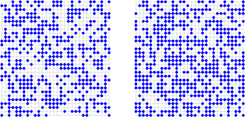
Figure 1: $2D$ site percolation. Shown are lattice realizations below (left) and above (right) the classical percolation threshold $p_{c}=0.592746$

For the quantum percolation problem all one-particle states are localized below the classical percolation threshold $p_{c}$, of course. Furthermore for arbitrary concentrations of conducting sites $p>p_{c}$ there always exist localized states on the infinite spanning cluster KE72 . Since for a completely ordered system ($p=1$) all states are extended and no states are extended for $p<p_{c}$, one might expect a disorder-induced Anderson transition at some critical concentration $p_{q}$, with $p_{c}\leq p_{q}\leq 1$. The reason is that the quantum nature of particles makes it harder for them to pass through narrow channels, despite the fact that quantum particles may tunnel through classically forbidden regions VW92 . As yet the existence of a quantum percolation threshold, different from the classical one, is discussed controversial, in particular for the two-dimensional ($2D$) case where also weak localization effects might become important LS96 .

Localization and quantum percolation have been the subject of much recent research; for a review of the more back dated work see e.g. Od86 ; LR85 . The underlying Anderson model (with uniformly distributed local potentials) and site percolation or binary alloy models (with a bimodal distribution of the on-site energies) are the two standard models for disordered solids. Although both problems have much in common, they differ in the type of disorder, and the localization phenomena of electrons in substitutional alloys are found to be much richer than previously claimed. For instance, the binary alloy model exhibits not one, as the $3D$ Anderson model, but several pairs of mobility edges, separating localized from extended states KE72 ; SWF05 ; AF05 . Moreover it appears that ‘forbidden energies’ exist, in the sense that near the band center the density of states continuously goes to zero. These effects might be observed in actual experiments.

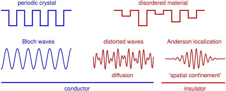
Figure 2: Anderson transition in disordered systems

Understanding these issues is an important task which we will address in this tutorial-style review by a stochastic approach that allows for a comprehensive description of disorder on a microscopic scale. This approach, which we call the local distribution (LD) approach AF05 ; AF06 , considers the local density of states (LDOS), which is a quantity of primary importance in systems with prominent local interactions or scattering. What makes the LD approach ‘non-standard’ is that it directly deals with the distribution of the LDOS in the spirit that Anderson introduced in his pioneering work An58 . While the LDOS is just related to the amplitude of the electron’s wave function on a certain lattice site, its distribution captures the fluctuations of the wave function through the system.

The present paper will be organized as follows. After introducing the basic concepts of the LD approach in Sect. 2 and explaining how to calculate the LDOS via the highly efficient Kernel Polynomial Method (KPM), we exemplify the LD concept by a study of localization within the Anderson model. Then, having all necessary tools at hand, we proceed in Sect. 3 to the problem of quantum percolation. Refining previous studies of localization effects in quantum percolation, we will demonstrate the ‘fragmentation’ of the spectrum into extended and localized states. The existence of a quantum percolation threshold is critically examined. To this end, we investigate for the $2D$ site-percolation problem the dynamical properties of an initially localized wave packet on the spanning cluster, using Chebyshev expansion in the time domain. In Sect. 4 we apply the findings to several classes of advanced materials where transport is related to percolating current patterns. Here prominent examples are $2D$ undoped graphene and the $3D$ colossal magnetoresistive manganites. Finally, in Sect. 5 we conclude with a short summary of the topic.

2 Local Distribution Approach

2.1 Conceptional background

In the theoretical investigation of disordered systems it turned out that the distribution of random quantities takes the center stage An58 ; AAT73 . Starting from a standard tight-binding Hamiltonian of noninteracting electrons on a $D$-dimensional hyper-cubic lattice with $N=L^{D}$ sites, the effect of compositional disorder in a solid may be described by site-dependent local potentials $\epsilon_{j}$.

$${H}=-t\sum\limits_{\langle ij\rangle}\bigl{(}{c}_{i}^{{\dagger}}{c}_{j}+\text{H.c.}\bigr{)}+\sum\limits_{j=1}^{N}\epsilon_{j}{c}_{j}^{{\dagger}}{c}_{j}\;.$$ (1)

The operators ${c}_{j}^{{\dagger}}$ (${c}_{j}$) create (annihilate) an electron in a Wannier state centered at site $j$, the on-site potentials $\epsilon_{j}$ are drawn from some probability distribution $p[\epsilon_{j}]$, and $t$ denotes the nearest-neighbor hopping element. While all characteristics of a certain material are determined by the corresponding distribution $p[\epsilon_{j}]$, we have to keep in mind, that each actual sample of this material constitutes only one particular realization $\{\epsilon_{j}\}$. The disorder in the potential landscape breaks translational invariance, which normally can be exploited for the description of ordered systems. Hence, we have to focus on site-dependent quantities like the LDOS at lattice site $i$,

$$\rho_{i}(E)=\sum\limits_{n=1}^{N}|\langle i|n\rangle|^{2}\,\delta(E-E_{n})\;,$$ (2)

where $|n\rangle$ is an eigenstate of $H$ with energy $E_{n}$ and $|i\rangle=c^{{\dagger}}_{i}|0\rangle$. Probing different sites in the crystal, $\rho_{i}(E)$ will strongly fluctuate, and recording the values of the LDOS we may accumulate the distribution $f[\rho_{i}(E)]$. In the thermodynamic limit, taking into account infinitely many lattice sites, the shape of $f[\rho_{i}(E)]$ will be independent of the actual realization of the on-site potentials $\{\epsilon_{j}\}$ and the chosen sites, but depend solely on the underlying distribution $p[\epsilon_{j}]$. Thus, in the sense of distributions, we have restored translational invariance, and the study of $f[\rho_{i}(E)]$ allows us to discuss the complete properties of the Hamiltonian (1). The probability density $f[\rho_{i}(E)]$ was found to have essentially different properties for extended and localized states MF94 . For an extended state the amplitude of the wave function is more or less uniform. Accordingly $f[\rho_{i}(E)]$ is sharply peaked and symmetric about the (arithmetically averaged) mean value $\rho_{\rm me}(E)$. On the other hand, if states become localized, the wave function has considerable weight only on a few sites. In this case the LDOS strongly fluctuates throughout the lattice and the corresponding LDOS distribution is mainly concentrated at $\rho_{i}=0$, very asymmetric and has a long tail. The rare but large LDOS-values dominate the mean value $\rho_{\rm me}(E)$, which therefore cannot be taken as a good approximation of the most probable value of the LDOS. Such systems are referred to as ‘non-self-averaging’. In numerical calculations, this different behavior may be used to discriminate localized from extended states in the following manner: Using the KPM with a variable number of moments for different interval sections (see Sect. 2.2) we calculate the LDOS for a large number of samples, $K_{r}$, and sites, $K_{s}$. Note that from a conceptual point of view, it makes no difference if we calculate $f[\rho_{i}(E)]$ for one large sample and many sites or consider smaller (but not too small) systems and more realizations of disorder. As the latter procedure is numerically more favorable, we will revert to this. Next, we sort the LDOS values for all energies within a small window around the desired energy $E$ into a histogram. As the LDOS values vary over several orders of magnitude, a logarithmic partition of the histogram presents itself. Although this procedure allows for the most intuitive determination of the localization properties in the sense of Anderson An58 , there are two drawbacks. First, to achieve a reasonable statistics, in particular for the slots at small LDOS values, a huge number of realizations is necessary. To alleviate the problems of statistical noise, it is advantageous to look at integral quantities like the distribution function

$$F[\rho_{i}(E)]=\int_{0}^{\rho_{i}(E)}f[\rho^{\prime}_{i}(E)]\,\mathrm{d}\rho^{\prime}_{i}(E)\;,$$ (3)

which also allows for the determination of the localization properties. While for extended states the more or less uniform amplitudes lead to a steep rise of $F[\rho_{i}]$, for localized states the increase extends over several orders of magnitude. Second, for practical calculations the recording of the whole distribution (or distribution function) is a bit inconvenient, especially if we want to discuss the localization properties of the whole band. Therefore we try to capture the main features of the distribution by comparing two of its characteristic quantities, the (arithmetically averaged) mean DOS,

$$\rho_{\text{me}}(E)=\frac{1}{K_{r}K_{s}}\smash{\sum\limits_{k=1}^{K_{r}}\sum\limits_{i=1}^{K_{s}}\rho_{i}(E)}\;,$$ (4)

and the (geometrically averaged) so called ‘typical’ DOS ,

$$\rho_{\text{ty}}(E)=\exp\left(\frac{1}{K_{r}K_{s}}\smash{\sum\limits_{k=1}^{K_{r}}\sum\limits_{i=1}^{K_{s}}\ln\bigl{(}\rho_{i}(E)\bigr{)}}\right)\;.$$ (5)

The typical DOS puts sufficient weight on small values of $\rho_{i}$. Therefore comparing $\rho_{\rm ty}(E)$ and $\rho_{\rm me}(E)$ allows to detect the localization transition. We classify a state at energy $E$ with $\rho_{\rm me}(E)\neq 0$ as localized if $\rho_{\rm ty}(E)=0$ and as extended if $\rho_{\rm ty}(E)\neq 0$. This method has been applied successfully to the pure Anderson model DPN03 ; SWWF05 ; ASWBF05 and even to more complex situations, where the effects of correlated disorder SWF05b , electron-electron interaction DK97 ; BHV05 or electron-phonon coupling BF02 ; BAF04 were taken into account.

2.2 Calculation of the Local Density of States by the Variable Moment Kernel Polynomial Method

At first glance, (2) suggests that the calculation of the LDOS could require a complete diagonalization of $H$. It turns out, however, that an expansion of $\rho_{i}$ in terms of a finite series of Chebyshev polynomials $T_{n}(x)=\cos(n\arccos x)$ allows for an incredibly precise approximation WWAF06 . Since the Chebyshev polynomials form an orthogonal set on $[-1,1]$, prior to an expansion the Hamiltonian $H$ needs to be rescaled, $\tilde{H}=(H-b)/a$. For reasons of numerical stability, we choose the parameters $a$ and $b$ such that the extreme eigenvalues of $\tilde{H}$ are $\pm 0.99$. In this way, the outer parts of the interval, where the strong oscillations of $T_{n}(x)$ can amplify numerical errors, contain no physical information and may be discarded. In terms of the coefficients, the so called Chebyshev moments,

$$\mu_{m}=\int\limits_{-1}^{1}\rho_{i}(x)T_{m}(x)\,\mathrm{d}x=\sum\limits_{n=1}^{N}\langle i|n\rangle\langle n|T_{m}(x_{n})|i\rangle=\langle i|T_{m}({\tilde{H}})|i\rangle\;,$$ (6)

the approximate LDOS reads

$$\rho_{i}(x)=\frac{1}{\pi\sqrt{1-x^{2}}}\left(g_{0}\mu_{0}+2\sum\limits_{m=1}^{M-1}g_{m}\mu_{m}T_{m}(x)\right)\;.$$ (7)

The Gibbs damping factors

$$g_{m}=\left(1-\frac{m\phi}{\pi}\right)\cos(m\phi)+\frac{\phi}{\pi}\sin(m\phi)\cot(\phi)$$ (8)

with $\phi=\pi/(M+1)$, are introduced to damp out the Gibbs oscillations resulting from finite-order polynomial approximations. The introduction of these factors corresponds to convoluting the finite series with the so called Jackson kernel SRVK96 . In essence, a $\delta$-peak at position $x_{0}$ is approximated by an almost Gaussian of width WWAF06

$$\sigma=\sqrt{\frac{M-x_{0}^{2}(M-1)}{2(M+1)}\left(1-\cos(2\phi)\right)}\approx\frac{\pi}{M}\sqrt{1-x_{0}^{2}+\frac{4x_{0}^{2}-3}{M}}\;.$$ (9)

Thus for a fixed number of moments, $M$, the resolution of the expansion gets better towards the interval boundaries. While in most applications this feature is harmless or even useful, here a uniform resolution throughout the whole band is mandatory to discriminate resolution effects from localization. This gets clear, if we respect that a small value of $\rho_{i}$ at a certain energy may either be due to a true low amplitude of the wave function, or to the absence of any energy level for the current disorder realization within one kernel width. Depending on which part of the interval we want to reconstruct, we need to restrict the used number of moments in (7) accordingly to ensure a constant $\sigma$. We call this procedure the Variable Moment KPM (VMKPM). The resulting approximations of a series of $\delta$-peaks using the standard KPM and the VMKPM, respectively, are compared in Fig. 3.

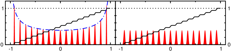
Figure 3: Approximation of a series of equally weighted $\delta$-peaks using the standard KPM (left) and the VMKPM (right). While both methods reproduce the correct spectral weight (solid line), only in the latter case a uniform resolution is obtained, reflected by the equal height of the peaks. The dashed-dotted line in the left panel is a guide to the eye being proportional to the inverse of the resolution (9)

For practical calculation of the moments, we may profit from the recursion relations of the Chebyshev polynomials,

$$T_{m+1}(x)=2xT_{m}(x)-T_{m-1}(x)\;,$$ (10)

starting from $T_{0}(x)=1$ and $T_{1}(x)=x$, and calculate the $\mu_{m}$ iteratively. Additionally, we may reduce the numerical effort by another factor $1/2$ by generating two moments with each matrix vector multiplication by ${\tilde{H}}$,

$$\begin{split}\mu_{2m-1}&=2\langle i|T_{m}({\tilde{H}})T_{m-1}({\tilde{H}})|i\rangle-\mu_{1}\;,\\ \mu_{2m}&=2\langle i|T_{m}({\tilde{H}})T_{m}({\tilde{H}})|i\rangle-\mu_{0}\;.\end{split}$$ (11)

Note that the algorithm requires storage only for the sparse matrix ${\tilde{H}}$ and two vectors of the corresponding dimension. Having calculated the desired number of moments, we calculate several reconstructions (7) for different $M$. We obtain the final result with uniform resolution by smoothly joining the corresponding results for the different subintervals. As the calculation of the $\mu_{m}$ dominates the computational effort, the additional overhead for performing several reconstructions is negligible as they can be done using a Fast Fourier Transform (FFT) routine.

2.3 Illustration of the Method: Anderson Localization in $3D$

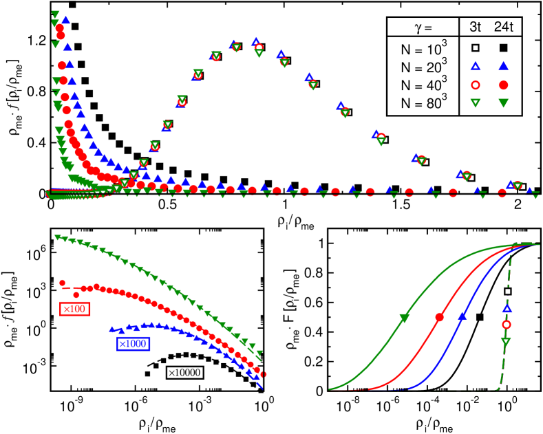
Figure 4: Upper panel: Finite-size scaling of the normalized LDOS distribution $f[\rho_{i}/\rho_{\text{me}}]$ at the band center ($|E|\leq 0.01t$) for the Anderson model. For the different system sizes $N$ we adapted the resolution $\sigma$ such that $N\sigma\approx 6.14$ is constant and calculated $10^{6},10^{4},1024,400$ realizations of $\rho_{i}$ for $N=10^{3},20^{3},40^{3},80^{3}$. Lower left panel: Double-logarithmic plot of $f[\rho_{i}/\rho_{\text{me}}]$ for the localized case together with log-normal fits (13) to the data. Note that for better visibility the data for $N=40^{3},20^{3},10^{3}$ were shifted vertically by $2,3,4$ orders of magnitude towards smaller values. Right lower panel: Distribution function $F[\rho_{i}/\rho_{\text{me}}]$ of the above data

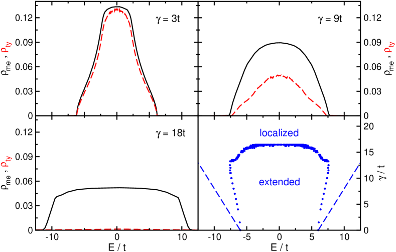
Figure 5: Mean (solid) and typical (dashed) density of states of the $3D$ Anderson model on a lattice with $N=60^{3}$ sites and periodic boundary conditions (PBC) for different values of disorder $\gamma$. We used $N\sigma=45$ and the shown curves result from an ensemble of $2000$ individual LDOS spectra obtained for different sites and realizations of disorder. Lower right panel: Mobility edge (dots) as obtained for $(\rho_{\text{ty}}/\rho_{\text{me}})_{c}=0.05$ and Lifshitz boundaries (dashed line)

To clarify the power of the method, let us briefly apply it to the Anderson model of localization An58 , for which the principal results are well known and can be found in the literature KM93_2 ; LR85 . The Anderson model is described by the Hamiltonian (1), using local potentials $\epsilon_{j}$, which are assumed to be independent, uniformly distributed random variables,

$$p[\epsilon_{j}]=\frac{1}{\gamma}\;\theta\left(\frac{\gamma}{2}-|\epsilon_{j}|\right)\;,$$ (12)

where the parameter $\gamma$ is a measure for the strength of disorder. The spectral properties of the Anderson model have been carefully analyzed (see e.g. FMSS85 ). For sufficiently large disorder or near the band tails, the spectrum consists exclusively of discrete eigenvalues, and the corresponding eigenfunctions are exponentially localized. Since localized electrons do not contribute to the transport of charge or energy, the energy that separates localized and extended eigenstates is called the mobility edge. For any finite amount of disorder $\gamma>0$, on a $1D$ lattice, all eigenstates of the Anderson Hamiltonian are localized Bo63 ; MT61 . This is believed to hold also in $2D$, where the existence of a transition from localized to extended states at finite $\gamma$ would contradict the one parameter scaling theory AALR79 ; Ja98 . In three dimensions, the disorder strength has a more distinctive effect on the spectrum. Only above a critical value $\gamma_{c}$ all states are localized, whereas for $\gamma<\gamma_{c}$ a pair of mobility edges separates the extended states in the band center from the localized ones near the band edges Mo67 . For this reason, the $3D$ case serves as a prime example on which we demonstrate how to discriminate localized from extended states within the local distribution approach. In the upper panel of Fig. 4 we show the resulting distribution of $\rho_{i}(E=0)$, normalized by its mean value $\rho_{\text{me}}$, for two characteristic values of disorder. As $\rho_{\text{me}}$ is a function of disorder, this normalization ensures $\langle\rho_{i}/\rho_{\text{me}}\rangle=1$ independent of $\gamma$, allowing for an appropriate comparison. In the delocalized phase, $\gamma=3t$, the distribution is rather symmetric and peaked close to its mean value. Note that increasing both the system size and VMKPM resolution, such that the ratio of mean level spacing to the width of the Jackson kernel is fixed, does not change the distribution. This is in strong contrast to the localized phase, $\gamma=24t$, where the distribution of $\rho_{i}(E)$ is extremely asymmetric. Although most of the weight is now concentrated close to zero, the distribution extends to very large values of $\rho_{i}$, causing the mean value to be much larger than the most probable value. Performing a similar finite-size scaling underlines both the asymmetry and the singular behavior which we expect for infinite resolution in the thermodynamic limit. Note also, that for the localized case, the distribution of the LDOS is extremely well approximated by a log-normal distribution MS83 ,

$$\Phi_{\text{log}}(x)=\frac{1}{\sqrt{2\pi\sigma_{0}^{2}}}\frac{1}{x}\exp\left(-\frac{\left(\ln\left(x/x_{0}\right)\right)^{2}}{2\sigma_{0}^{2}}\right)\;,$$ (13)

as illustrated in the lower left panel of Fig. 4. The shifting of the distribution towards zero for localized states is most obvious in the distribution function $F[\rho_{i}]$ which is depicted in the lower right panel of Fig. 4. While for extended states the more or less uniform amplitudes lead to a steep rise of $F[\rho_{i}]$, for localized states the increase extends over several orders of magnitude. Capturing the essential features of the LDOS distribution by concentrating on the mean ($\rho_{\text{me}}$) and typical ($\rho_{\text{ty}}$) density of states, we determine the localization properties for the whole energy band depending on the disorder. As can be seen from Fig. 5, $\rho_{\text{me}}(E)$ and $\rho_{\text{ty}}(E)$ are almost equal for extended states, whereas for localized states $\rho_{\text{ty}}(E)$ vanishes while $\rho_{\text{me}}(E)$ remains finite. Using the well-established value $\gamma_{c}(E=0)\simeq 16.5t$ as a calibration for the critical ratio $\rho_{\text{ty}}/\rho_{\text{me}}$, required to distinguish localized from extended states for the used system size and resolution, we reproduce the mobility edge in the energy-disorder plane MK83 ; KM93_2 ; GS95 (see lower right panel of Fig. 5). We also find the well-known re-entrant behavior near the unperturbed band edges BSK87 ; Qu01 : Varying $\gamma$ for some fixed values of $E$ ($6t<E\leq 7.6t$) a region of extended states separates two regions of localized states. The Lifshitz boundaries, shown as dashed lines, indicate the energy range, where eigenstates are in principle allowed. As the probability of reaching the Lifshitz boundaries is exponentially small, we cannot expect to find states near these boundaries for the finite ensembles considered in any numerical calculation.

3 Localization Effects in Quantum Percolation

In disordered solids the percolation problem is characterized by the interplay of pure classical and quantum effects. Besides the question of finding a percolating path of ‘accessible’ sites through a given lattice, the quantum nature of the electrons imposes further restrictions on the existence of extended states and, consequently, of a finite DC-conductivity.

As a particularly simple model we start again from the basic Hamiltonian (1) drawing the $\{\epsilon_{j}\}$ from the bimodal distribution

$$p[\epsilon_{j}]=p\,\delta(\epsilon_{j}-\epsilon_{A})+(1-p)\,\delta(\epsilon_{j}-\epsilon_{B})\;.$$ (14)

The two energies $\epsilon_{A}$ and $\epsilon_{B}$ could, for instance, represent the potential landscape of a binary alloy A_pB_1-p, where each site is occupied by an $A$ or $B$ atom with probability $p$ or $1-p$, respectively. Therefore we call (1) together with the distribution (14) the binary alloy model. In the limit $\Delta=(\epsilon_{B}-\epsilon_{A})\rightarrow\infty$ the wave function of the $A$ sub-band vanishes identically on the $B$-sites, making them completely inaccessible for the quantum particles. We then arrive at a situation where non-interacting electrons move on a random ensemble of $\tilde{N}$ lattice points, which, depending on $p$, may span the entire lattice or not. The corresponding quantum site percolation model reads

$${H}=-t\!\sum_{\langle ij\rangle\in A}\!({c}_{i}^{{\dagger}}{c}_{j}+\text{H.c.})\;,$$ (15)

where the summation extends over nearest-neighbor $A$-sites only and, without loss of generality, $\epsilon_{A}$ is chosen to be zero.

Within the classical percolation scenario the percolation threshold $p_{c}$ is defined by the occurrence of an infinite cluster $A_{\infty}$ of connected $A$ sites. For the simple cubic lattice this site-percolation threshold is $p_{c}^{3D}=0.311609$ BFMSPR99 for the $3D$ case and $p_{c}^{2D}=0.592746$ NZ00 in $2D$. In the quantum case, the multiple scattering of the particles at the irregular boundaries of the cluster can suppress the wave function, in particular within narrow channels or close to dead ends of the cluster. Hence, this type of disorder can lead to absence of diffusion due to localization, even if there is a classical percolating path through the crystal. On the other hand, for finite $\Delta$ the tunneling between $A$ and $B$ sites may cause a finite DC-conductivity although the $A$ sites are not percolating. Naturally, the question arises whether the quantum percolation threshold $p_{q}$, given by the probability above which an extended wave function exists within the $A$ sub-band, is larger or smaller than $p_{c}$. Previous results SLG92 ; NBR02 for finite values of $\Delta$ indicate that the tunneling effect has a marginal influence on the percolation threshold as soon as $\Delta\gg 4tD$.

3.1 $3D$ Site Percolation

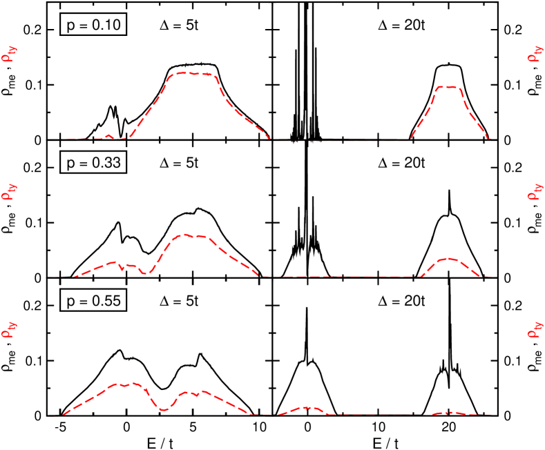
Figure 6: Mean (upper solid line) and typical (lower dashed line) DOS of the binary alloy model on a $N=64^{3}$ lattice with PBC for different concentrations of $A$-sites $p$ and local potential differences $\Delta$. Taking all sites into account, we chose the resolution such that $N\sigma=45$ and calculated $1000$ individual LDOS spectra for different probe realizations and sites

Before discussing possible localization phenomena let us investigate the behavior of the mean DOS for the binary alloy and quantum percolation model in $3D$. Figure 6 shows that as long as $\epsilon_{A}$ and $\epsilon_{B}$ do not differ too much there exists a single and if $p\neq 0.5$ asymmetric electronic band SLG92 . At about $\Delta\simeq 4tD$ this band separates into two sub-bands centered at $\epsilon_{A}$ and $\epsilon_{B}$, respectively. The most prominent feature in the split-band regime is the series of spikes at discrete energies within the band. As an obvious guess, we might attribute these spikes to eigenstates on islands of $A$ or $B$ sites being isolated from the main cluster KE72 ; BA96 . It turns out, however, that some of the spikes persist, even if we neglect all finite clusters and restrict the calculation to the $\bar{N}$ sites of $A$-type on the spanning cluster, $A_{\infty}$. This is illustrated in the upper panels of Fig. 7, where we compare the DOS of the binary alloy model at $\Delta\to\infty$ and the quantum percolation model. Increasing the concentration of accessible sites the mean DOS of the spanning cluster is evocative of the DOS of the simple cubic lattice, but even at large values of $p$ a sharp peak structure remains at $E=0$ (see Fig. 7, lower panels).

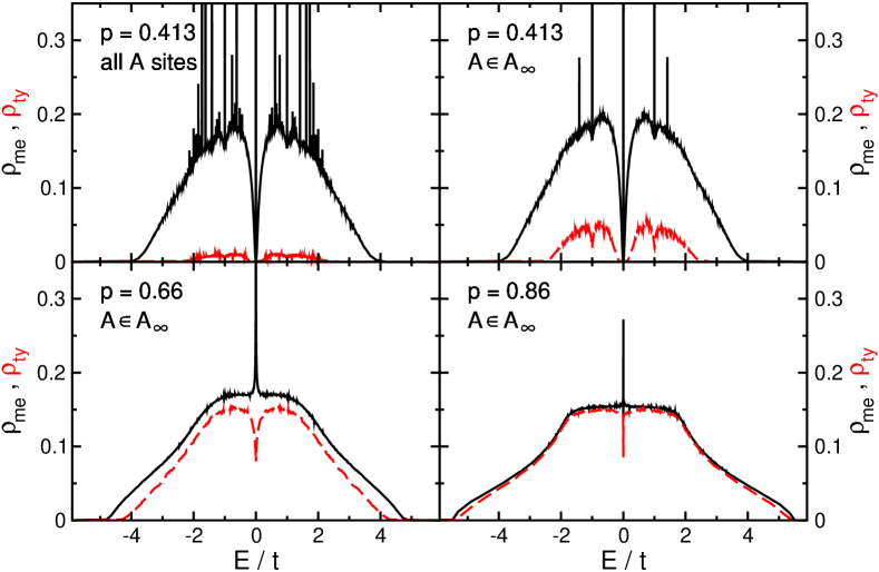
Figure 7: Mean (solid line) and typical (dashed line) DOS for the quantum percolation model in the limit $\Delta\to\infty$. While in the upper left panel all $A$-sites are taken into account, the other three panels show data for the restricted model on the spanning cluster $A_{\infty}$ only (note that $\rho_{\rm ty}$ is smaller in the former case because there are more sites with vanishing amplitude of the wave function). Using $\sigma=0.0002$, we adapt the system sizes to ensure $\bar{N}\sigma=45$ for the $A_{\infty}$ case, i.e. , $N=64^{3},70^{3},84^{3}$ for $p=0.86,0.66,0.413$. For the case of all $A$ sites at $p=0.413$, $N=82^{3}$ guarantees $\tilde{N}\sigma=45$. For each system, we consider $512$ individual LDOS spectra for different sites and realizations of disorder

To elucidate this effect, which for a long time was partially not accounted for in the literature KE72 ; SLG92 ; OOM80 ; SEG87 , in more detail, in Fig. 8 we fix $p$ at $0.337$, shortly above the classical percolation threshold. In addition to the most dominant peaks at $E/t=0,\pm 1,\pm\sqrt{2}$, we can resolve distinct spikes at $E/t=\frac{1}{2}\left(\pm 1\pm\sqrt{5}\right),\pm\sqrt{3},\pm\sqrt{2\pm\sqrt{2}},\ldots$ . These special energies coincide with the eigenvalues of the tight-binding model on small clusters of the geometries shown in the right part of Fig. 8. In accordance with KE72 and CCFST86 we can thus argue that the wave functions, which correspond to these special energies, are localized on some ‘dead ends’ of the spanning cluster.

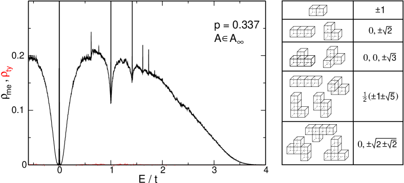
Figure 8: Left: Mean (solid line) and typical (dashed line) DOS for the quantum percolation model with $p=0.337$ on a $N=100^{3}$ lattice (restriction to $A_{\infty}$, PBC, $\bar{N}\sigma=45$). The data are an ensemble average over 1000 realizations of disorder and different sites. Note that $\rho_{\text{ty}}<10^{-3}$ holds in the whole band. Right: Some cluster configurations related to the special energies at which the peaks in $\rho_{\text{me}}$ occur

The assumption that the distinct peaks correspond to localized wave functions is corroborated by the fact that the typical DOS vanishes or, at least, shows a dip at these energies. Occurring also for finite $\Delta$ (Fig. 6), this effect becomes more pronounced as $\Delta\to\infty$ and in the vicinity of the classical percolation threshold $p_{c}$. From the study of the Anderson model we know that localization leads at first to a narrowing of the energy window containing extended states. For the percolation problem, in contrast, with decreasing $p$ the typical DOS indicates both localization from the band edges and localization at particular energies within the band. Since finite cluster wave functions like those shown in Fig. 8 can be constructed for numerous other, less probable geometries Sc03 , an infinite discrete series of such spikes might exist within the spectrum, as proposed in CCFST86 . The picture of localization in the quantum percolation model is then quite remarkable. If we generalize our numerical data for the peaks at $E=0$ and $E=\pm t$, it seems as if there is an infinite discrete set of energies with localized wave functions, which is dense within the entire spectrum. In between there are many extended states, but to avoid mixing, their density goes to zero close to the localized states. Facilitated by its large special weight (up to 11% close to $p_{c}$) this is clearly observable for the peak at $E=0$, and we suspect similar behavior at $E=\pm t$. For the other discrete spikes the resolution of our numerical data is still too poor and the system size might be even too small to draw a definite conclusion.

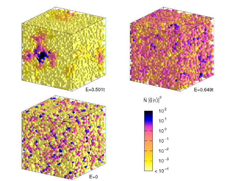
Figure 9: Normalized probability density $\bar{N}|\langle i|n\rangle|^{2}$ for three eigenstates of the quantum percolation model. The chosen energies are representative for a localized ($E=3.501t$), extended ($E=0.649t$) and anomalous localized ($E=0$) state. We performed an exact diagonalization for $A_{\infty}$ for one realization of disorder on a $N=32^{3}$ lattice with PBC and $p=0.458$

In order to understand the internal structure of the extended and localized states we calculate the probability density of specific eigenstates of (15) restricted to $A_{\infty}$ for a fixed realization of disorder. Figure 9 visualizes the spatial variation of $|\langle i|n\rangle|^{2}$ for an occupation probability well above the classical percolation threshold. The figure clearly indicates that the state with $E=0.649t$ is extended, i.e. the spanning cluster is quantum mechanically ‘transparent’. On the contrary, at $E=3.501t$, the wave function is completely localized on a finite region of the spanning cluster. This is caused by the scattering of the particle at the random surface of the spanning cluster.

A particularly interesting behavior is observed at $E=0$. Here, the eigenstates are highly degenerate and we can form wave functions that span the entire lattice in a checkerboard structure with zero and non-zero amplitudes (see Fig. 9). Although these states are extended in the sense that they are not confined to some region of the cluster, they are localized in the sense that they do not contribute to the DC-conductivity. This is caused by the alternating structure which suppresses the nearest-neighbor hopping, and in spite of the high degeneracy, the current matrix element between different $E=0$ states is zero. Hence, having properties of both classes of states these states are called anomalously localized SAH82 ; ITA94 . Another indication for the robustness of this feature is its persistence for mismatching boundary conditions, e.g., periodic (anti-periodic) boundary conditions for odd (even) values of the linear extension $L$. In these cases the checkerboard is matched to itself by a manifold of sites with vanishing amplitude.

Furthermore for the previously mentioned special energies, the wave function vanishes identically except for some finite domains on loose ends (like those shown in the right panel of Fig. 8), where it takes, except for normalisation, the values ($\pm 1,\mp 1$), ($1,\pm\sqrt{2},1$), ($-1,0,1$), $\ldots$ Note that these regions are part of the spanning cluster, connected to the rest of $A_{\infty}$ by sites with wave function amplitude zero CCFST86 .

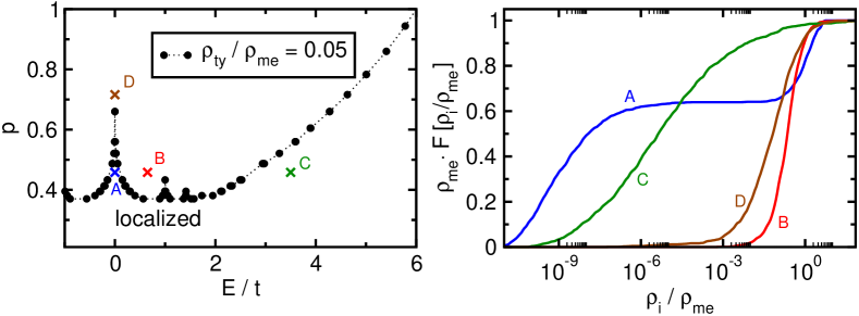
Figure 10: Left panel: Normalized typical DOS $\rho_{\rm ty}/\rho_{\rm me}$ in the concentration-energy plane for the quantum percolation model restricted to $A_{\infty}$. For a fixed resolution of $\sigma=0.0002$ we adapted the system sizes to keep $\bar{N}\sigma=45$ constant, i.e., $N=62^{3},\ldots,120^{3}$ for $p=0.944,\ldots,0.318$. The results base on the calculation of 1000 individual LDOS spectra for different cluster realizations and sites. Right panel: Distribution function of the LDOS for four characteristic states, for which the parameters $(p,E)$ are indicated by crosses in the left panel. The parameters for the curves $A,B,C$ are the same for which we showed the characteristic states in Fig. 9

In the past most of the methods used in numerical studies of Anderson localization have also been applied to the binary alloy model and the quantum percolation model in order to determine the quantum percolation threshold $p_{q}$, defined as the probability $p$ below which all states are localized (see, e.g., MDS95 ; KN90 and references therein). The existence of $p_{q}$ is still disputed. As yet the results for $p_{q}$ are far less precise than, e.g., the values of the critical disorder reported for the Anderson model. For the simple cubic lattice numerical estimates of quantum site-percolation thresholds range from 0.4 to 0.5 (see KN90 and references therein). In Figs. 6-8 we present data for $\rho_{\rm ty}$ which shows that $p_{q}>p_{c}$. In fact, within numerical accuracy, we found $\rho_{\rm ty}=0$ for $p=0.337>p_{c}$.

To get a more detailed picture we calculate the normalized typical DOS, $\rho_{\rm ty}/\rho_{\rm me}$, in the whole concentration-energy plane. The left panel of Fig. 10 presents such kind of phase diagram of the quantum percolation model. This data also supports a finite quantum percolation threshold $p_{q}\stackrel{{\scriptstyle>}}{{\sim}}0.4>p_{c}$ (see also SLG92 ; KN90 ; KSHS97 ; KO99 ), but as the discussion above indicated, for $E=0$ and $E=\pm t$ the critical value $p_{q}(E)=1$, and the same may hold for the set of other ‘special’ energies. The transition line between localized and extended states, $p_{q}(E)$, might thus be a rather irregular (fractal?) function. On the basis of our LDOS distribution approach, however, we are not in the position to answer this question with full rigor.

Finally let us come back to the characterization of extended and localized states in terms of distribution functions. The right panel of Fig. 10 displays the distribution function, $F[\rho_{i}(E)]$, for four typical points in the energy-concentration plane, corresponding to localized, extended, and anomalously localized states, respectively. The differences in $F[\rho_{i}(E)]$ are significant. The slow increase of $F[\rho_{i}(E)]$ observed for localized states corresponds to an extremely broad LDOS-distribution, with a very small most probable (or typical) value of $\rho_{i}(E)$. This is in agreement with the findings for the Anderson model. Accordingly the jump-like increase found for extended states is related to an extremely narrow distribution of the LDOS centered around the mean DOS, where $\rho_{\rm me}$ coincides with the most probable value. At $E=0$ and low $p$, the distribution function exhibits two steps, leading to a bimodal distribution density. Here the first (second) maximum is related to sites with a small (large) amplitude of the wave function – a feature that substantiates the checkerboard structure discussed above. For higher $p$, where we already found a reduced spectral weight of the central peak in $\rho_{\text{me}}$, also the two step shape of the distribution function is less pronounced. Therefore we may argue, the increase in weight of the central peak for lower $p$ is substantially due to the checkerboard states.

Having a rather complete perception of the physics in $3D$, let us now come to the $2D$ case, for which the findings in literature are more controversial.

3.2 $2D$ Site Percolation

Although the main characteristics of the $3D$ site-percolation problem, e.g., the fragmentation of the spectrum, persist in $2D$, there exist some particularities and additional difficulties. In particular, the existence of a quantum percolation threshold $1>p_{q}>p_{c}=0.592746$ is even less settled than in $3D$. Published estimates range from $p_{q}=p_{c}$ to $p_{q}=1$ (see KN90 ; IN07p and references therein). This uncertainty is due to the extremely large length scales, on which localization phenomena take place in $2D$, a fact well-known for the standard Anderson model. Furthermore the special characteristics of the band center states seem to be of particular importance ITA94 ; ERS98b .

Local Density of States

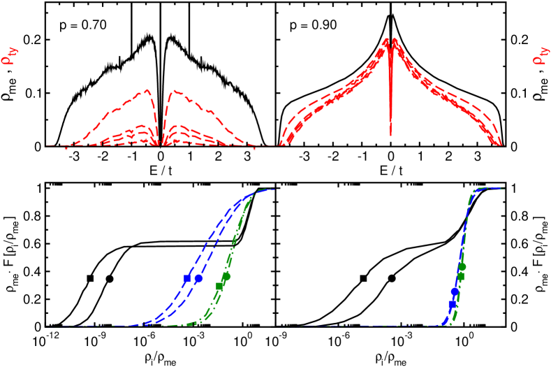
Figure 11: Upper panels: Mean (solid line) and typical (dashed lines) DOS for the $2D$ percolation model for $p=0.7$ (left) and $p=0.9$ (right). The dashed lines correspond to the typical DOS for different system sizes (from top to bottom) $N=114^{2},400^{2},572^{2},1144^{2}$ for $p=0.7$ and $N=100^{2},350^{2},500^{2},1000^{2}$ for $p=0.9$. Again, we adapt $\sigma$, such that $\bar{N}\sigma=45$. The curves are ensemble averages over $1000$ ($500$ for the largest systems) individual LDOS spectra for different cluster realizations and sites. Lower panel: Distribution function of the LDOS for three characteristic energies: $E=0$ (solid lines), $E=0.5t$ (dashed-dotted lines), and $E=2.5t$ (dashed lines). To underline the finite size scaling, we show the results for two system sizes, $350^{2}$ ($400^{2}$) marked with circles, and $500^{2}$ ($572^{2}$) with squares

Figure 11 shows the mean and typical DOS of the $2D$ quantum percolation model, calculated by the LD approach. For large $p$, $\rho_{\text{me}}$ clearly resembles the $2D$ DOS shape for the ordered case. For these parameters $\rho_{\text{ty}}$ nearly coincides with $\rho_{\text{me}}$ except for the band center, where $\rho_{\text{ty}}$ shows a strong dip. If we reduce the occupation probability, the spikes at special energies appear again (see Sect. 3.1), with most spectral weight at $E=0$. The weight of the central peak (9% close to $p_{c}$) is reduced as compared to the $3D$ case.

In order to obtain reliable results for the infinite system, we examine the dependency of $\rho_{\text{ty}}$ on the system size, for fixed $\bar{N}\sigma$. Here, we find a characteristic difference between large and small $p$. Whereas for large $p$, above a certain system size, $\rho_{\text{ty}}$ is independent of $N$, it continuously decreases for low occupation probabilities. This behavior is evocative of extended and localized states, respectively. Taking a look at the underlying distribution functions, we find a similar situation as in the $3D$ case. At $E=0$, the two level distribution evolves, indicating the checkerboard structure of the state. Away from the special energies, the distribution function exhibits the shape characteristic for extended and localized states. This behavior exposes when we compare $F[\rho_{i}(E)]$ for different system sizes. Whereas for extended states the distribution function is insensitive against this scaling, it shifts towards smaller values for localized ones.

Although these results are quite encouraging, one aspect deserves further attention. If we try to calculate the LDOS distribution at a given energy $E$, due to the finite resolution of the KPM, it will also contain contributions from states in the vicinity of $E$. Thus taking the fragmentation of the spectrum into localized and extended states seriously, the LDOS distribution within this artificial interval will contain contributions of each class of states.

For practical calculations, this causes no problems, as except for the most pronounced peaks, the probability of finding a state which is localized on one of the geometries like in the right panel of Fig. 8 drops very fast with its complexity.

Time Evolution

The expansion of the time evolution operator $U(\tau)=\mathrm{e}^{-{\rm i}H\tau}$ in Chebyshev polynomials allows for a very efficient method to calculate the dynamics of a quantum system. We may profit from this fact by calculating the recurrence probability of a particle to a given site, $P_{R}(\tau)$, which for $\tau\to\infty$ may serve as a criterion for localization Ja98 ; KM93_2 . While for extended states on the spanning cluster $P_{R}(\tau\to\infty)=1/\bar{N}$, which scales to zero in the thermodynamic limit, a localized state will have a finite value of $P_{R}(\tau)$ as $\bar{N}\to\infty$. The advantage of considering the time evolution is that in general the initial state is not an eigenstate of the system and therefore contains contributions of the whole spectrum. This allows for a global search for extended states and a detection of $p_{q}$.

Let us briefly outline how to calculate the time evolution of the system by means of Chebyshev expansion TK84 ; CG99 . Of course, as a first step, the Hamiltonian has to be rescaled to the definition interval of the Chebyshev polynomials, leading to

$$U(\tau)=\mathrm{e}^{-{\rm i}(a\tilde{H}+b)\tau}=\mathrm{e}^{-{\rm i}b\tau}\left[c_{0}+2\sum\limits_{k=1}^{M}c_{k}T_{k}(\tilde{H})\right]\;.$$ (16)

The expansion coefficients $c_{k}$ are given by

$$c_{k}=\int\limits_{-1}^{1}\dfrac{T_{k}(x)e^{-{\rm i}ax\tau}}{\pi\sqrt{1-x^{2}}}\mathrm{d}x=(-{\rm i})^{k}J_{k}(a\tau)\;,$$ (17)

where $J_{k}$ denotes the Bessel function of the first kind. Due to the fast asymptotic decay of the Bessel functions

$$J_{k}(a\tau)\sim\frac{1}{k!}\left(\frac{a\tau}{2}\right)^{k}\sim\frac{1}{\sqrt{2\pi k}}\left(\frac{\mathrm{e}a\tau}{2k}\right)^{k}\quad\text{for}\quad k\to\infty\;,$$ (18)

the higher-order expansion terms vanish rapidly. Thus we do not need additional damping factors as in the Chebyshev expansion of the LDOS, but may truncate the series at some order without having to expect Gibbs oscillations. Note that the expansion order necessary to obtain precise results will surely depend on the time step used, normally $M\sim 2at$ will be sufficient. Thus, for optimum performance of the algorithm, we have to find a suitable compromise between time step $\Delta\tau$ and expansion order $M$. Anyhow, for reasonable $M$, the method permits the use of larger time steps compared to the standard Crank-Nicolson algorithm.

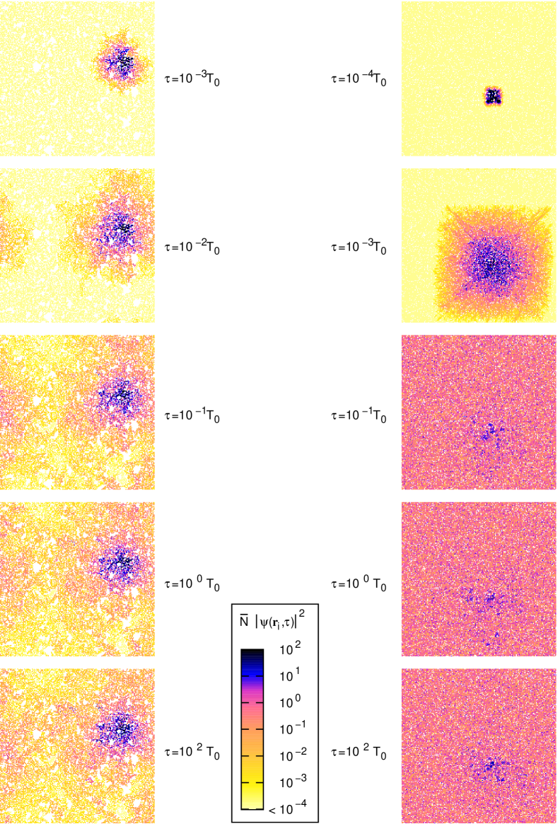
Figure 12: Time evolution of a state at $E=0.5t$ on the spanning cluster of a $N=200^{2}$ lattice for $p=0.65$ (left) and $p=0.90$ (right). We show the normalized square of the wave function amplitude at the different sites $\bar{N}|\psi({\mathbf{r}}_{i},\tau)|^{2}$ . Due to this normalization, for an extended state which is evenly spread over all sites of $A_{\infty}$ this quantity is equal to unity

Having this powerful tool at hand, we are now in the position to calculate how $\psi({\mathbf{r}}_{i},\tau)$ evolves on $A_{\infty}$ in time. The ’natural’ time scales of the system are given by the energy of the nearest-neighbor hopping element $\tau_{0}=1/t$, describing one hopping event, and the time a particle needs (in a completely ordered system) to visit each site once, $T_{0}=N\tau_{0}$. As initial state, we prepare a completely localized state, whose amplitude vanishes exactly, except for two neighboring sites, where it has amplitudes $a$ and $\sqrt{1-a^{2}}$, respectively. For this state we can calculate the energy $E=2ta\sqrt{1-a^{2}}$ and, choosing $a$ appropriately, we may continuously tune $E\in[-t,t]$. Taking into account more complicated initial configurations of occupied sites (see right panel in Fig. 8) we may also adjust higher energies. For each starting position, however, the local structure of $A_{\infty}$ limits the possible configurations.

In Fig. 12 we compare the time evolution of a state for high and low occupation probability $p$, for which qualitatively different behaviors emerge. For $p=0.65$, the wave function is localized on a finite region of the cluster. Following the time evolution up to very long times ($>100T_{0}$) we demonstrate that this is not just a transitional state during the spreading process of the wave function, but true ’dynamical’ localization. This behavior is in strong contrast to $p=0.90$, where the state spreads over the whole cluster within a short fraction of this time ($0.1T_{0}$). For any fixed time there are some sites with slightly larger amplitudes (the darker dots in the last image of the time series). Those are due to contributions from localized states which are also present in the initial state. However, as the wave function extends over the whole cluster, for large $p$ not all states in the spectum may be localized. Since the time evolution of initial states at $p=0.65$ and $p=0.90$ behaves in such a different manner, we conclude that there exists a quantum percolation threshold in between.

Consequently, we have a method at hand, capable to visualize the dynamical properties of localization in quantum percolation SF08 .

4 Percolative Effects in Advanced Materials

Current applications of quantum percolation concern e.g. transport properties of doped semiconductors ITA94 and granular metals FIS04 , metal-insulator transition in 2D n-GaAs heterostructures SLHPWR05 , wave propagation through binary inhomogeneous media AL92 , superconductor-insulator and (integer) quantum Hall transitions DMA04 ; SMK03 , or the dynamics of atomic Fermi-Bose mixtures SKSZL04 . Another important example is the metal-insulator transition in perovskite manganite films and the related colossal magnetoresistance (CMR) effect, which in the meantime is believed to be inherently percolative BSLMDSS02 . Quite recently (quantum) percolation models have been proposed to mimic the minimal conductivity in undoped graphene CFAA07p . In doped graphene, in the split-band regime, an internal mobility edge might appear around the Fermi energy by introducing impurities Na07p . Moreover, geometric disorder is shown to strongly affect electronic transport in graphene nanoribbons MB07p . In the remaining part of this paper we exemplarily investigate two specific random resistor network models to describe qualitatively charge transport in graphene sheets and bulk manganites.

4.1 Graphene

Due to its remarkable electronic properties, recently a lot of activity has been devoted to graphene, the atomic mono/bi-layer modification of graphite NGMJZDGF04 ; NMMFKZJSG06 ; GN07 . Especially the gapless spectrum with linear dispersion near the Fermi energy and the possibility of continuously varying the charge carrier density (from n- to p- type) by means of applying a gate voltage are of technological interest. In view of possible applications, like graphene-based field effect transistors, it is highly desirable to know how these characteristics change in the presence of disorder, inherent in any prepared probe. Therefore much work has been dedicated to study possible localization effects due to the presence of disorder (cf. PGLPC06 and references therein).

The extraordinary electronic structure of graphene results in unusual transport properties. In this material a finite minimal conductivity is observed, which might be attributed to a mesoscopically inhomogeneous density of charge carriers Ge06 ; MAULSVY07p ; CF07p , caused by spatially varying charge trapping on the substrate. To describe the influence of these charge inhomogeneities on the transport properties, percolative random resistor networks (RRN) have been proposed CFAA07p . Following this line, we apply the LD approach to a minimal model SF08b that can be constructed in generalization of the $2D$ percolation model described in Sect. 3.2.

Let us consider a $2D$ lattice on which the sublattices represent regions of different charge carrier concentrations. These regions (sites) are randomly connected with each other (left panel of Fig. 13).

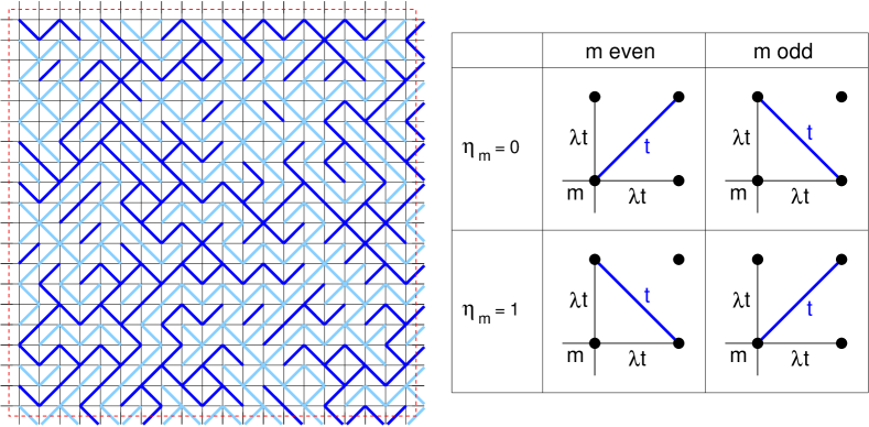
Figure 13: Left panel: One particular cluster realization of the RRN model at $p=0.5$. Right panel: Visualization of the generation rule for the RRN model

The hopping probability for such links (to some next nearest neighbors) is assumed to be much higher than for direct nearest neighbor hopping events. The later ones are reduced by the leakage, $\lambda$, as compared to the others. To examine the influence of anisotropic hopping, we model the corresponding RRN by the Hamiltonian

$$\begin{split}H=-t\Big{[}\lambda\sum\limits_{m}\left(c^{{\dagger}}_{m}c_{n}+c^{{\dagger}}_{m}c_{e}\right)+\sum\limits_{m\;\text{even}}\left(\eta_{m}c^{{\dagger}}_{m}c_{ne}+(1-\eta_{m})c^{{\dagger}}_{e}c_{n}\right)+\\ +\sum\limits_{m\;\text{odd}}\left(\eta_{m}c^{{\dagger}}_{e}c_{n}+(1-\eta_{m})c^{{\dagger}}_{m}c_{ne}\right)\Big{]}+\text{H.c.}\;,\end{split}$$ (19)

where $e$(ast) and $n$(orth) denote the nearest neighbors of site $m$ in $x$- and $y$-direction and $ne$ is the next-nearest neighbor in ‘north-east’ direction. We assume PBC. The random variable $\eta_{m}\in\{0,1\}$ determines which diagonal in a square is connected (right panel in Fig. 13). Shifting the expectation value of the $\{\eta_{m}\}$, we may adjust the anisotropy of the system $p=\langle\eta_{m}\rangle$. While the link directions are isotropically distributed for $p=0.5$, increasing (decreasing) $p$ generates a preferred direction of hopping, favoring stripe-like structures. Note that in the limit of vanishing leakage this model is equivalent to the $2D$ percolation model discussed in Sect. 3.

First representative results for the RRN model are presented in Fig. 14. In particular it shows the influence of finite leakage and anisotropy. In contrast to the $2D$ percolation model, where the DOS spectra are completely symmetric, the inclusion of next-nearest neighbor hopping causes an asymmetry that grows with increasing $\lambda$. For large $p$, the mean DOS is evocative of the $1D$ DOS, except for the multitude of spikes, which we can attribute again to localized states on isolated islands. In the isotropic, low-leakage case, a vanishing $\rho_{\text{ty}}$ suggests that all states are localized. Either increasing $p$ or $\lambda$ leads to a finite value of $\rho_{\text{ty}}$. But even at $p=0.90$ this effect is marginal for small $\lambda$, thus presumably no extended states exist. Increasing the leakage results in a finite $\rho_{\text{ty}}$ for $E>0$ also at $p=0.5$. This feature becomes even more pronounced at high anisotropy, which indicates the existence of extended states for these parameters.

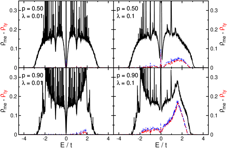
Figure 14: Mean (solid line) and typical (dashed line) DOS for the RRN model. Results are shown for $N=500^{2}$ and $N\sigma=45$ for different anisotropy $p$ and leakage $\lambda$. For illustration of the finite size dependence, $\rho_{\text{ty}}$ for a $N=350^{2}$ sites system is also included (dotted lines). The results base on the calculation of 1000 individual LDOS spectra for different cluster realizations and sites

In Fig. 15 we present some characteristic eigenstates of this model for a fixed realization of disorder. These results support the conclusions drawn from the typical DOS. For the isotropic, low-leakage case we find a clearly localized state with internal checkerboard structure. Increasing the anisotropy, many states are extended in one direction (cf. the $1D$-like shape of $\rho_{\text{me}}$), while localized in the other one. The leakage has a more drastic effect on the nature of the states, as they are extended in some sense for both values of $p$. The amplitudes on different lattice sites fluctuate over several orders of magnitude, however, explaining the reduced value of $\rho_{\text{ty}}$ as compared to $\rho_{\text{me}}$ (cf. Fig 14).

Due to the simplicity of the model, these results are surely not suitable to be compared to real experimental transport data, but can be seen as a first step towards an at least qualitative understanding of the extraordinary transport properties in graphene. In any case, also here the LD approach may serve as a reliable tool to discuss localization effects.

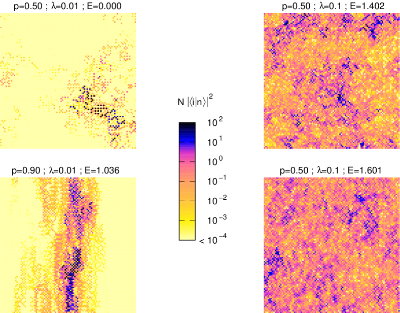
Figure 15: Characteristic eigenstates of the RRN model on a $N=100^{2}$ lattice at different anisotropies $p$, leakage rates $\lambda$, and energies $E$. Shown is the normalized occupation probability $N|\langle i|n\rangle|^{2}$

4.2 Doped CMR Manganites

The transition from a metallic ferromagnetic (FM) low-temperature phase to an insulating paramagnetic high-temperature phase observed in some hole-doped manganese oxides (such as the perovskite family $\rm La_{1-x}[Sr,Ca]_{x}MnO_{3}$) is associated with an unusual dramatic change in their electronic and magnetic properties. This includes a spectacularly large negative magnetoresistive response to an applied magnetic field (see Fig. 16, left panel), which might have important technological applications JTMFRC94 .

Recent experiments indicate the coexistence of localized and itinerant charge carriers close to the metal-insulator transition in the FM phase of CMR manganites. Above $T_{c}$ the activated behaviour of the conductivity WMG98 as well as the structure of the pair distribution function (PDF) BDKNT96 indicate the formation of small polarons, i.e., of almost localized carriers within a surrounding lattice distortion. Interestingly these polarons continue to exist in the metallic phase below $T_{c}$, merely their volume fraction is noticeable reduced. For the coexistence of conducting and insulating regions within the metallic phase different scenarios were discussed, which relate the metal-insulator transition to phase separation DHM01 and percolative phenomena GK98 ; MMFYD00 . In particular microscopic imaging techniques, like scanning tunneling spectroscopy FFMTAM99 ; Beea02 or dark-field imaging UMCC99 , seem to support the latter idea.

In previous work WLF03 we addressed this problem theoretically. We proposed a phenomenological mixed-phase description which is based on the competition of a polaronic insulating phase and a metallic, double-exchange driven ferromagnetic phase, whose volume fractions and carrier concentrations are determined self-consistently by requiring equal pressure and chemical potential. In more detail, we assume that the resistivity of the metallic component is proportional to the expression

$$\rho_{S}[z]=\frac{g_{S}[z]-\gamma_{S}[z]^{2}}{\gamma_{S}[z]^{2}}\,,\\$$ (20)

derived by Kubo and Ohata KO72a , which associates $\rho$ with the fluctuation of the double-exchange matrix element caused by the thermal spin disorder. Here $S=3/2$ is the localized spin formed by the $t_{2g}$ electrons of the manganese. Both,

$$g_{S}[z] =\frac{SB_{S}[z]}{(2S+1)^{2}}\left((2S+2)\coth\frac{(S+1)z}{S}-\coth\frac{z}{2S}\right)+\frac{S+1}{2S+1}$$ (21)

$$\gamma_{S}[z] =\frac{S+1}{2S+1}+\frac{S}{2S+1}\coth\left(\frac{S+1}{S}z\right)B_{S}[z]\;,$$ (22)

exhibit a magnetic field dependence, where $B_{S}[z]=\frac{1}{2S}\big{[}(2S+1)\coth\tfrac{(2S+1)z}{2S}-\coth\tfrac{z}{2S}\big{]}$. The resistivity of the insulating component is assumed to match the resistivity of the high-temperature phase, which in experiment is well fit by the activated hopping of small-polarons WMG98 . Hence, the resistivities of the two components are given by,

$$\rho^{(f)}=\frac{B}{x^{(f)}}\left(\rho_{S}[S(\lambda+\lambda^{\text{ext}})]+\rho_{\text{min}}\right)\quad\text{and}\quad\rho^{(p)}=\frac{A}{\beta x^{(p)}}\ \rho_{S}[S\lambda^{\text{ext}}]\ \mathrm{e}^{-\beta\epsilon_{p}}\;,$$ (23)

where $\epsilon_{p}$ is the polaron binding energy, $\beta=1/k_{B}T$ the inverse temperature, $\lambda$ is the inner Weiss field, $\lambda^{\text{ext}}$ ist the external magnetic field and the prefactors $A$ and $B$ as well as the cut-off $\rho_{\text{min}}$ are free model parameters which could be estimated from experimental data. Then, at a given doping level $x$, i.e. chemical potential $\mu$, the resulting carrier concentrations $x^{(f)}$ and $x^{(p)}$ in the coexisting regions define the two volume fractions by the equations

$$x=p^{(f)}x^{(f)}+p^{(p)}x^{(p)}\quad\text{and}\quad p^{(f)}+p^{(p)}=1\,,$$ (24)

(see WLF03 ). The resistivity of the whole sample, which may consist of an inhomogeneous mixture of both components, is calculated on the basis of a RRN. More precisely, we choose nodes from a cubic lattice which belong to the metallic component with probability $p^{(f)}$ and to the polaronic component with probability $p^{(p)}$. Each of these nodes, which represent macroscopic regions of the sample, is connected to its neighbours with resistors of magnitude $\rho^{(f)}$ or $\rho^{(p)}$, respectively.

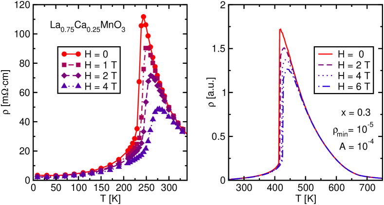
Figure 16: Experimental (left) and theoretical (right) results for the temperature- and magnetic field-dependence of the resistivity in doped CMR manganites. Experimental data are taken from Ref. SRBC95 . For a more detailed discussion see also WLF03

Inserting the volume fractions and carrier concentrations from the mixed-phase model we obtain the resistivities shown in Fig. 16 (right panel). The jump-like behaviour of the resistivity originates to a large degree from the changing volume fraction of the metallic component, which can cross the percolation threshold. However, the conductivity of the component itself as well as its carrier concentration strongly affect $\rho$ for $T<T_{c}$. An external magnetic field causes a reasonable suppression of $\rho$, i.e., a noticeable negative magnetoresistance. Compared to the real compounds the calculated effect is a bit weaker. Nevertheless, in view of the rather simple model for the conductivity the agreement is quite satisfactory. More involved assumptions, e.g. an affinity to the formation of larger regions of the same type in the sense of correlated percolation KK03 would naturally affect the resistivity of the system and its response to an external field.

5 Conclusions

In this tutorial we demonstrated the capability of the local distribution approach to the problem of quantum percolation. In disordered systems the local density of states (LDOS) emerges as a stochastic, random quantity. It makes sense to take this stochastic character seriously and to incorporate the distribution of the LDOS in a description of disorder. Employing the Kernel Polynomial Method we can resolve with very moderate computational costs the rich structures in the density of states originating from the irregular boundary of the spanning cluster.

As for the standard Anderson localization and binary alloy problems the geometrically averaged (typical) density of states characterizes the LDOS distribution and may serve as a kind of order parameter differentiating between extended and localized states. For both $2D$ and $3D$ quantum site percolation, our numerical data corroborate previous results in favor of a quantum percolation threshold $p_{q}>p_{c}$ and a fragmentation of the electronic spectrum into extended and localized states. At the band center, so called anomalous localization is observed, which manifests itself in a checkerboard-like structure of the wave function. Most notably, monitoring the spatial evolution of a wave packet in time for the $2D$ case, we find direct evidence for ’dynamical’ localization of an incident quantum particle at $p=0.65>p_{c}$, while its wave function is spread over the percolated cluster for $p=0.9$. This finding additionally supports the existence of a quantum percolation threshold.

Without a doubt quantum percolation plays an important role in the transport of several contemporary materials, such as $2D$ graphene or $3D$ manganese oxides. To close the gap between the study of simple percolation models and a realistic treatment of percolative transport in these rather complicated materials will certainly be a challenge of future research.

We thank A. Alvermann, F. X. Bronold, J. W. Kantelhardt, S. A. Trugman, A. Weiße, and G. Wellein for valuable discussions. This work was supported by the DFG through the research program TR 24, the Competence Network for Technical/Scientific High-Performance Computing in Bavaria (KONWIHR), and the Leibniz Computing Center (LRZ) Munich.

References

- (1) P.W. Anderson, Phys. Rev. 109, 1492 (1958)
- (2) B. Kramer, A. Mac Kinnon, Rep. Prog. Phys. 56, 1469 (1993)
- (3) S. Kirkpatrick, T.P. Eggarter, Phys. Rev. B 6, 3598 (1972)
- (4) D. Vollhardt, P. Wölfle, in Electronic Phase Transitions, ed. by W. Hanke, Y.V. Kopaev (North Holland, Amsterdam, 1992), p. 1
- (5) T. Li, P. Sheng, Phys. Rev. B 53, R13268 (1996)
- (6) T. Odagaki, in Transport and Relaxation in Random Materials, ed. by J. Klafter, R.J. Rubin, M.F. Shlesinger (World Scientific, Singapore, 1986)
- (7) P.A. Lee, T.V. Ramakrishnan, Rev. Mod. Phys. 57, 287 (1985)
- (8) G. Schubert, A. Weiße, H. Fehske, Phys. Rev. B 71, 045126 (2005)
- (9) A. Alvermann, H. Fehske, Eur. Phys. J. B 48, 295 (2005)
- (10) A. Alvermann, H. Fehske, J. Phys.: Conf. Ser. 35, 145 (2006)
- (11) R. Abou-Chacra, D.J. Thouless, P.W. Anderson, J. Phys. C 6, 1734 (1973)
- (12) A.D. Mirlin, Y.V. Fyodorov, J. Phys. I (France) 4, 655 (1994)
- (13) V. Dobrosavljević, A.A. Pastor, B.K. Nikolić, Europhys. Lett. 62, 76 (2003)
- (14) G. Schubert, A. Weiße, G. Wellein, H. Fehske, in High Performance Computing in Science and Engineering, Garching 2004, ed. by A. Bode, F. Durst (Springer-Verlag, Heidelberg, 2005), pp. 237–250
- (15) A. Alvermann, G. Schubert, A. Weiße, F.X. Bronold, H. Fehske, Physica B 359–361, 789 (2005)
- (16) G. Schubert, A. Weiße, H. Fehske, Physica B 359–361, 801 (2005)
- (17) V. Dobrosavljević, G. Kotliar, Phys. Rev. Lett. 78, 3943 (1997)
- (18) K. Byczuk, W. Hofstetter, D. Vollhardt, Phys. Rev. Lett. 94, 056404 (2005)
- (19) F.X. Bronold, H. Fehske, Phys. Rev. B 66, 073102 (2002)
- (20) F.X. Bronold, A. Alvermann, H. Fehske, Philos. Mag. 84, 673 (2004)
- (21) A. Weiße, G. Wellein, A. Alvermann, H. Fehske, Rev. Mod. Phys. 78, 275 (2006)
- (22) R.N. Silver, H. Röder, A.F. Voter, D.J. Kress, J. of Comp. Phys. 124, 115 (1996)
- (23) J. Fröhlich, F. Martinelli, E. Scoppola, T. Spencer, Commun. Math. Phys. 101, 21 (1985)
- (24) R.E. Borland, Proc. Roy. Soc. London, Ser. A 274, 529 (1963)
- (25) N.F. Mott, W.D. Twose, Adv. Phys. 10, 107 (1961)
- (26) E. Abrahams, P.W. Anderson, D.C. Licciardello, T.V. Ramakrishnan, Phys. Rev. Lett. 42, 673 (1979)
- (27) M. Janssen, Physics Reports 295, 1 (1998)
- (28) N.F. Mott, Adv. Phys. 16, 49 (1967)
- (29) E.W. Montroll, M.F. Shlesinger, J. Stat. Phys. 32, 209 (1983)
- (30) A. Mac Kinnon, B. Kramer, Z. Phys. B 53, 1 (1983)
- (31) H. Grussbach, M. Schreiber, Phys. Rev. B 51, 663 (1995)
- (32) B. Bulka, M. Schreiber, B. Kramer, Z. Phys. B 66, 21 (1987)
- (33) S.L.A. de Queiroz, Phys. Rev. B 653, 214202 (2001)
- (34) H.G. Ballesteros, L.A. Fernández, V. Martín-Mayor, G.P. A. Muiñoz Sudupe, J.J. Ruiz-Lorenzo, J. Phys. A 32, 1 (1999)
- (35) M.E.J. Newman, R.M. Ziff, Phys. Rev. Lett. 85, 4104 (2000)
- (36) C.M. Soukoulis, Q. Li, G.S. Grest, Phys. Rev. B 45, 7724 (1992)
- (37) H.N. Nazareno, P.E. de Brito, E.S. Rodrigues, Phys. Rev. B 66, 012205 (2002)
- (38) R. Berkovits, Y. Avishai, Phys. Rev. B 53, R16125 (1996)
- (39) T. Odagaki, N. Ogita, H. Matsuda, J. Phys. C 13, 189 (1980)
- (40) C.M. Soukoulis, E.N. Economou, G.S. Grest, Phys. Rev. B 36, 8649 (1987)
- (41) J.T. Chayes, L. Chayes, J.R. Franz, J.P. Sethna, S.A. Trugman, J. Phys. A 19, L1173 (1986)
- (42) G. Schubert, Numerische Untersuchung ungeordneter Elektronensysteme. diploma thesis, Universität Bayreuth (2003)
- (43) Y. Shapir, A. Aharony, A.B. Harris, Phys. Rev. Lett. 49, 486 (1982)
- (44) M. Inui, S.A. Trugman, E. Abrahans, Phys. Rev. B 49, 3190 (1994)
- (45) A. Mookerjee, I. Dasgupta, T. Saha, Int. J. Mod. Phys. B 9, 2989 (1995)
- (46) T. Koslowski, W. von Niessen, Phys. Rev. B 42, 10342 (1990)
- (47) A. Kusy, A.W. Stadler, G. Hałdaś, R. Sikora, Physica A 241, 403 (1997)
- (48) A. Kaneko, T. Ohtsuki, J. Phys. Soc. Jpn. 68, 1488 (1999)
- (49) M.F. Islam, H. Nakanishi, Phys. Rev. E 77, 061109 (2008)
- (50) A. Eilmes, R.A. Römer, M. Schreiber, Phys. Status Solidi B 205, 229 (1998)
- (51) H. Tal-Ezer, R. Kosloff, J. Chem. Phys. 81, 3967 (1984)
- (52) R. Chen, H. Guo, Comp. Phys. Comm. 119, 19 (1999)
- (53) G. Schubert, H. Fehske, Phys. Rev. B 77, 245130 (2008)
- (54) M.V. Feigel’mann, A. Ioselevich, M. Skvortsov, Phys. Rev. Lett. 93, 136403 (2004)
- (55) S. Das Sarma, M.P. Lilly, E.H. Hwang, L.N. Pfeiffer, K.W. West, J.L. Reno, Phys. Rev. Lett. 94, 136401 (2005)
- (56) Y. Avishai, J. Luck, Phys. Rev. B 45, 1974 (1992)
- (57) Y. Dubi, Y. Meir, Y. Avishai, Phys. Rev. B 71, 125311 (2005)
- (58) N. Sandler, H.R. Maei, J. Kondev, Phys. Rev. B 70, 045309 (2004)
- (59) A. Sanpera, A. Kantian, L. Sanchez-Palencia, J. Zakrzewski, M. Lewenstein, Phys. Rev. Lett. 93, 040401 (2004)
- (60) T. Becker, C. Streng, Y. Luo, V. Moshnyaga, B. Damaschke, N. Shannon, K. Samwer, Phys. Rev. Lett. 89, 237203 (2002)
- (61) V.V. Cheianov, V.I. Fal’ko, B.L. Altshuler, I.L. Aleiner, Phys. Rev. Lett. 99, 176801 (2007)
- (62) G.G. Naumis, Phys. Rev. B 76, 153403 (2007)
- (63) I. Martin, Y.M. Blanter, Transport in disordered graphene nanoribbons (2007). URL arXiv:0705.0532. (preprint)
- (64) K.S. Novoselov, A.K. Geim, S.V. Morozov, D. Jiang, Y. Zhang, S.V. Dubonos, I.V. Grigorieva, A.A. Firsov, Science 306, 666 (2004)
- (65) K.S. Novoselov, E. McCann, S.V. Morozov, V.I. Fal’ko, M.I. Katsnelson, U. Zeitler, D. Jiang, F. Schedin, A.K. Geim, Nature Phys. 2, 177 (2006)
- (66) A.K. Geim, K.S. Novoselov, Nature Mat. 6, 183 (2007)
- (67) V.M. Pereira, F. Guimea, J.M.B. Lopes dos Santos, N.M.R. Peres, A.H. Castro Neto, Phys. Rev. Lett. 96, 036801 (2006)
- (68) A.K. Geim, Nature Phys. 2, 620 (2006)
- (69) J. Martin, N. Akerman, G. Ulbricht, T. Lohmann, J.H. Smet, K. von Klitzing, A. Yacoby, Nature Phys. 4, 144 (2008)
- (70) S. Cho, M.S. Fuhrer, Phys. Rev. B 77, 081402(R) (2008)
- (71) G. Schubert, H. Fehske, Phys. Rev. B 78, 155115 (2008)
- (72) S. Jin, T.H. Tiefel, M. McCormack, R.A. Fastnach, R. Ramesh, L.H. Chen, Science 264, 413 (1994)
- (73) D.C. Worledge, L. Miéville, T.H. Geballe, Phys. Rev. B 57, 15267 (1998)
- (74) S.J.L. Billinge, R.G. DiFrancesco, G.H. Kwei, J.J. Neumeier, J.D. Thompson, Phys. Rev. Lett. 77, 715 (1996)
- (75) E. Dagotto, T. Hotta, A. Moreo, Physics Reports 344, 1 (2001)
- (76) L.P. Gor’kov, V.Z. Kresin, JETP Lett. 67, 985 (1998)
- (77) A. Moreo, M. Mayr, A. Feiguin, S. Yunoki, E. Dagotto, Phys. Rev. Lett. 84, 5568 (2000)
- (78) M. Fäth, S. Freisem, A.A. Menovsky, Y. Tomioka, J. Aarts, J.A. Mydosh, Science 285, 1540 (1999)
- (79) T. Becker, C. Streng, Y. Luo, V. Moshnyaga, B. Damaschke, N. Shannon, K. Samwer, Phys. Rev. Lett. 89, 237203 (2002)
- (80) M. Uehara, S. Mori, C.H. Chen, S.W. Cheong, Nature 399, 560 (1999)
- (81) A. Weiße, J. Loos, H. Fehske, Phys. Rev. B 68, 024402 (2003)
- (82) K. Kubo, N. Ohata, J. Phys. Soc. Jpn. 33, 21 (1972)
- (83) P. Schiffer, A.P. Ramirez, W. Bao, S.W. Cheong, Phys. Rev. Lett. 75, 3336 (1995)
- (84) D. Khomskii, L. Khomskii, Phys. Rev. B 67, 052406 (2003)
Index
- Anderson localization §2.3
- Anderson model §2.1
- binary alloy model §3
- Chebyshev expansion §3.2
- CMR effect §4
- fragmentation of the spectrum §3.2
- graphene §4, §4.1
- KPM §2.2
- LDOS §2.2
- local distribution approach §2
- mean DOS §2.1
- quantum site percolation model §3
- random resistor network §4.1
- RRN §4.1
- site percolation threshold §3
- time evolution §3.2
- typical DOS §2.1