Keck HIRES Spectroscopy of Extragalactic H II Regions: C and O Abundances from Recombination Lines

Abstract

We present very deep spectrophotometry of 14 bright extragalactic H II regions belonging to spiral, irregular, and blue compact galaxies. The data for 13 objects were taken with the HIRES echelle spectrograph on the Keck I telescope. We have measured C II recombination lines in 10 of the objects and O II recombination lines in 8 of them. We have determined electron temperatures from line ratios of several ions, specially of low ionization potential ones. We have found a rather tight linear empirical relation between $T_{\rm e}$([N II]) and $T_{\rm e}$([O III]). We have found that O II lines give always larger abundances than [O III] lines. Moreover, the difference of both O⁺⁺ abundance determinations –the so-called abundance discrepancy factor– is very similar in all the objects, with a mean value of 0.26 $\pm$ 0.09 dex, independently of the properties of the H II region and of the parent galaxy. Using the observed recombination lines, we have determined the O, C, and C/O radial abundance gradients for 3 spiral galaxies: M 33, M 101, and NGC 2403, finding that C abundance gradients are always steeper than those of O, producing negative C/O gradients accross the galactic disks. This result is similar to that found in the Milky Way and has important implications for chemical evolution models and the nucleosynthesis of C.

1 Introduction

The spectral analysis of H II regions allows the determination of the chemical composition of the ionized gas-phase of the interstellar medium from the solar neighbourhood to the high-redshift Universe. Therefore, it stands as an essential tool for our knowledge of the chemical evolution of the Universe. With the advent of 8-10 m class ground-based telescopes, we can now obtain extremely deep spectra of extragalactic H II regions (hereafter EHRs). These new studies have permitted, for example, to obtain direct determinations of the electron temperature, $T_{\rm e}$, in high-metallicity EHRs (see Bresolin, 2008, and references therein), where the auroral lines become very faint, or to measure recombination lines (hereafter RLs) useful for abundance determinations of heavy-element ions (Peimbert, 2003; López-Sánchez et al., 2007; Bresolin, 2007).

The detection of C II and O II lines produced by pure recombination in EHRs was firstly reported by Esteban et al. (2002) from deep spectra taken with the 4.2 m William Herschel Telescope. In principle, these lines have the advantage that their intensity is much less dependent on the value of $T_{\rm e}$ than the collisionally excited lines (hereafter CELs), which are the lines commonly used for abundance determinations in nebulae. The brightest C II RL is C II $\lambda$4267, with typical fluxes of the order of 10^-3 $\times$ $I$(H$\beta$). This line permits to derive the C⁺⁺ abundance, which is the dominant ionization stage of C for the typical conditions of EHRs. There are only a few C abundance determinations available for EHRs, most of them derived from UV CELs that can only be observed from space (Garnett et al., 1995, 1999; Kobulnicky & Skillman, 1998), and more recently from RLs (Esteban et al., 2002; Peimbert, 2003; Tsamis et al., 2003; Peimbert et al., 2005; López-Sánchez et al., 2007; Bresolin, 2007). The C abundance determinations based on UV CELs are severely affected by uncertainties in the reddening correction. To further complicate the situation, the STIS spectrograph aboard the Hubble Space Telescope, the only instrument capable to detect the UV CELs of C in bright EHRs, stopped science operations in 2004, so that nowadays the observation of the optical CII RLs provides the only possibility for determining C abundances in EHRs. The study of the behavior of C/H and C/O ratios and their galactocentric gradients in galaxies of different morphological types and metallicities is of paramount importance and can provide observational constraints for a better knowledge of the nucleosynthetic origin of carbon –the most important biogenic element– as well as the star formation/enrichment timescales in galaxies (e.g. Carigi et al., 2005).

O⁺⁺ is the only ion that simultaneously shows bright CELs and detectable –relatively bright– RLs in the optical range. In H II regions, the O⁺⁺ abundances derived from RLs are always between 0.10 and 0.35 dex higher than those derived from CELs (see compilation by García-Rojas & Esteban, 2007). This observational fact is currently known as the “abundance discrepancy” (hereafter AD) problem. We define the abundance discrepancy factor (hereafter ADF) as the logarithmic difference between the abundance derived from RLs and CELs:

$${\rm ADF}({\rm X}^{i+})={\rm log}({\rm X}^{i+}/{\rm H}^{+})_{\rm RLs}-{\rm log}({\rm X}^{i+}/{\rm H}^{+})_{\rm CELs},$$ (1)

where Xⁱ⁺ corresponds to the ionization state $i$ of element X. Although the ADF found in H II regions is remarkably constant, this is not the case for planetary nebulae, PNe, where the values of the ADF can be quite different from object to object, with the ADFs ranging from near zero up to ten in some extreme cases (e.g. Liu, 2006). This different behaviour led García-Rojas & Esteban (2007) to the conclusion that the mechanism that produces the AD –or the bulk of it– in the extreme PNe should be different to that producing the AD in H II regions. The fact that the determination of nebular abundances is still uncertain, by at least a factor of two, has an important impact on many astrophysical aspects, such as chemical evolution and nucleosynthesis models and predictions, as well as the calibration of the so-called “strong line methods” used to estimate abundances in local and high-redshift star-forming galaxies. This last point was recently highlighted by Peimbert et al. (2007).

The origin of the AD problem is still object of debate and a challenge for our understanding of ionized nebulae. The results for a sample of Galactic H II regions seem to be consistent with the predictions of the temperature fluctuations paradigm (García-Rojas & Esteban, 2007). In fact, in the presence of temperature fluctuations (parameterized by the mean square of the spatial variations of temperature, the $t^{\rm 2}$ parameter) the AD can be naturally explained because of the different temperature dependence of the intensity of RLs and CELs. However, the presence of temperature fluctuations in ionized nebulae still lacks a direct demonstration. An alternative explanation for the origin of the AD has been proposed by Tsamis & Péquignot (2005) and Stasińska et al. (2007), which is based on the presence of cold high-metallicity clumps of supernova ejecta still not mixed with the ambient gas of the H II regions. This cold gas would produce most of the emission of the RLs whereas the ambient gas of normal abundances would emit most of the intensity of CELs. However, López-Sánchez et al. (2007), who detect C II and O II lines in the dwarf galaxy NGC 5253, question this hypothesis in the light of the results available for EHRs.

Our group is interested in exploring the physical process that control the AD as well as in determining C abundances and radial gradients. In this paper, we make use of deep high-resolution spectrophotometry of a sample of bright EHRs in spiral and irregular galaxies as well as some giant H II regions in dwarf galaxies –H II galaxies– in order to explore a wide range of metallicities, H II regions of different sizes and structure, and galaxy morphological types. We think that this kind of study is necessary, mainly because the only intermediate-resolution spectral study devoted for the detection of RLs in EHRs of spiral galaxies was that by Esteban et al. (2002), which only included –apart from NGC 2363 in the irregular galaxy NGC 2366– three objects in two spirals (one in M 33 and two in M 101).

A highlight of this work is the use of high-spectral resolution spectrophotometry. These data are needed to increase the contrast between the faint RLs and the continuum, to deblend the O II lines of multiplet 1, and to separate them properly from possible Wolf-Rayet emission features as well as absorption features due to underlying stellar populations.

In §§ 2 and 3 of this paper we describe the observations, the data reduction procedure, the measurement of the emission lines, and the derivation of the reddening coefficient. In § 4 we derive the physical conditions of the nebulae and explore the consistency of different temperature scales, as well as calculate the ionic abundances from both kinds of lines: CELs and RLs. In § 5 we discuss the ADF in the sample objects and the radial C, O, and C/O abundance gradients in the spiral galaxies M 33, M 101, and NGC 2403. Finally, in § 6 we summarize our main conclusions.

2 Observations and Data Reduction

The observations of the sample objects, except NGC 5447 –a bright H II region in the galaxy M 101– were made on 2006 April 20 and 21 and November 14 with the High Resolution Echelle Spectrometer (HIRES, Vogt et al., 1994) at the Keck I telescope on Mauna Kea Observatory. The spectra cover the 3550–7440 Å range with a somewhat discontinuous wavelength coverage due to gaps between the detectors and to the fact that the redmost spectral orders do not fit completely within the CCD. The decker D3 was used, covering an area of 7$\farcs$0 $\times$ 1$\farcs$7. This configuration provides a spectral resolution of R=23,000. We observed a single slit position for each object. The center and position angle of the slits were chosen to cover the maximum area of the brightest part of the objects and the final usable one-dimensional spectra were extracted from an area of 5$\farcs$76 $\times$ 1$\farcs$7 for all the objects. The journal of the observations is shown in Table 1. The table includes the coordinates of the centers of the slits. In the case of the H II regions belonging to spiral galaxies with two or more objects observed –M33, NGC 2403, and M101, all of morphological type Sc– we also include the galactocentric distance (in kpc) and $R$/$R_{0}$ ratio of each H II region. The adopted distances to the galaxies have been taken from Freedman et al. (2001), and are 0.84, 3.22, and 7.5 Mpc for M33, NGC 2403, and M101, respectively. For M33, we have considered the photometric radius, $R_{0}$, of 28′ estimated by de Vaucouleurs et al. (1976), an inclination angle of 56^∘, and a position angle of 23^∘ (Zaritsky et al., 1989). In the case of NGC 2403, we have adopted $R_{0}$ = 8$\farcm$5 (Zaritsky et al., 1994), $i$ = 60^∘, and PA = 126^∘ (Garnett et al., 1997). Finally, for M101 we have assumed $R_{0}$ = 14$\farcm$4 (de Vaucouleurs et al., 1991), $i$ = 18^∘, and PA = 37^∘ (Kamphuis, 1993).

Intermediate-resolution spectroscopy of NGC 5447 was obtained on 2008 May 11 with the ISIS spectrograph at the 4.2m William Herschel Telescope (WHT) of the Observatorio del Roque de los Muchachos (La Palma, Spain). Two different CCDs were used at the blue and red arms of the spectrograph: an EEV CCD with a configuration 4100 $\times$ 2048 pixels with a pixel size of 13.5 $\mu$m in the blue arm and a REDPLUS CCD with 4096 $\times$ 2048 pixels with a pixel size of 15 $\mu$m in the red arm. The dichroic prism used to separate the blue and red beams was set at 5300 Å. The slit was 3$\farcm$7 long and 1$\farcs$03 wide. Two gratings were used, the R1200B in the blue arm and the R316R in the red arm. These gratings give reciprocal dispersions of 17 and 62 Å mm^-1, and effective spectral resolutions of 0.86 and 3.56 Å for the blue and red arms, respectively. The blue spectra cover from $\lambda\lambda$4225 to 5075 Å and the red ones from $\lambda\lambda$5430 to 8195 Å. The one-dimensional spectra were extracted from an area of 3$\farcs$2 $\times$ 1$\farcs$03, corresponding to the brighest zone of NGC 5447.

Standard data reduction procedures, including bias correction, flat-fielding, order extraction, wavelength calibrations, and flux calibration, were carried out using routines in the ECHELLE and ONEDSPEC packages of IRAF. The correction for atmospheric extinction was performed using the average curve for continuous atmospheric extinction at Mauna Kea and Roque de los Muchachos. The absolute flux calibration was achieved by observations of the standard stars Feige 34, Feige 66, Feige 110, H600, BD+25 4655, and BD+28 4211 in the case of the observations taken with the Keck I telescope and Feige 34, BD+25 3941, and BD+33 2624 in the case of the observations taken with the WHT.

Table 1: Journal of observations

									Exposure
Host		R.A.	Decl.	$R_{\rm G}$		Date of		P.A.	Time
Galaxy	Object	(J2000.0)	(J2000.0)	(kpc)	$R$/$R_{0}$	Observation	Telescope	(deg)	(s)
M31	K932	00 46 34.0	+42 11 51	$\cdots$	$\cdots$	14/11/2006	Keck	330	3$\times$1800
M33	NGC 595	01 33 34.2	+30 41 38	2.87	0.42	14/11/2006	Keck	90	3$\times$1800
M33	NGC 604	01 34 33.3	+30 46 47	4.11	0.60	14/11/2006	Keck	90	3$\times$1200
NGC 1741	Zone C	05 01 37.6	$-$04 15 30	$\cdots$	$\cdots$	14/11/2006	Keck	50	2$\times$1200
NGC 2366	NGC 2363	07 28 42.7	+69 11 26	$\cdots$	$\cdots$	20/04/2006	Keck	220	3$\times$1800
NGC 2403	VS 24	07 36 45.7	+65 36 55	1.00	0.126	14/11/2006	Keck	295	3$\times$1500
NGC 2403	VS 38	07 36 51.8	+65 36 42	1.04	0.131	14/11/2006	Keck	275	3$\times$1650
NGC 2403	VS 44	07 37 06.8	+65 36 41	2.77	0.346	14/11/2006	Keck	330	3$\times$1500
NGC 4395	Region #70	12 25 57.7	+33 31 32	$\cdots$	$\cdots$	21/04/2006	Keck	330	3$\times$1800
NGC 4861	Brightest HII region	12 59 00.1	+34 50 37	$\cdots$	$\cdots$	20/04/2006	Keck	220	3$\times$1800
M83	Nucleus	13 36 59.8	$-$29 52 07	$\cdots$	$\cdots$	21/04/2006	Keck	90	3$\times$1800
M101	H1013	14 03 32.2	+54 21 10	5.50	0.19	20/04/2006	Keck	270	4$\times$1800
M101	NGC 5461	14 03 41.0	+54 19 01	9.84	0.34	20/04/2006	Keck	225	3$\times$1800
M101	NGC 5447	14 02 28.7	+54 16 25	16.21	0.56	11/05/2008	WHT	134	7$\times$1800

3 Line intensities and Reddening Correction

Line intensities were measured integrating all the flux in the line between two given limits and over a local continuum estimated by eye. In the cases of line blending, a multiple Gaussian profile fit procedure was applied to obtain the line flux of each individual line. The measurements were performed with the SPLOT routine of the IRAF package.

Figure 1: Sections of the spectra of NGC 604 (upper panels), K932 (middle panels), and NGC 2363 (lower panels) showing the C II $\lambda$4267 (left) recombination line and the lines of multiplet 1 of O II $\sim$$\lambda$$\lambda$4650 (right).

Table 2 and Table 3 show the emission-line intensities measured for 10 EHRs where the RLs of O II and/or C II have been detected. Table 4 includes the emission-line intensities for 4 objects where those RLs were not detected. Due to their relevance to this paper, upper limits of the intensities of C II $\lambda$4267 and/or O II $\lambda$4649 –one of the brightest lines of multiple 1 of O II– at 1 $\sigma$ level have been estimated and included in the tables for the objects where those RLs were not detected. For M 83, we cannot estimate appropriate upper limits of the intensities of C II and O II lines due to the contamination of spectral features produced by the underlying stellar emission to the continuum at low intensities. The first column of tables 2 to 4 includes the adopted laboratory wavelength, $\lambda_{0}$, of the line. The second and third columns include the ion and identification of the line. The fourth column lists the reddening curve used (Seaton, 1979). The following columns include –one pair of columns for each object– the observed wavelength in the heliocentric rest frame, $\lambda$, and the reddening-corrected flux relative to H$\beta$, $I$($\lambda$), of the lines. The identification and adopted laboratory wavelength of the lines, as well as the error analysis applied, were obtained following García-Rojas et al. (2004), adding quadratically the error due to flux calibration that has been estimated to be 1 and 3 per cent for the November and April 2006 Keck I observations, respectively, and 4 per cent for the WHT observations. This flux calibration error corresponds to the standard deviation obtained from the calibration curves of the standard stars observed in each run. Colons indicate line flux errors of the order or greater than 40%.

A number of lines between 38 (M83-Nucleus) and 135 (NGC 2363) have been measured in the spectra of the 14 objects included in this study. A substantial fraction of them are permitted lines of heavy-element ions: C II, N I, O I, O II, and Si II; of these, only C II $\lambda$4267 and the lines of multiplet 1 of O II at $\sim$$\lambda\lambda$4650 are pure RLs and can be used for abundance determinations. The rest of the permitted lines are mainly produced by fluorescence mechanisms (see Esteban et al., 2004). Only a small fraction of the lines are dubious identifications or could not be identified. Figure 1 contains sections of the spectra of three of the sample objects –NGC 604, K932 and NGC 2363– showing the C II $\lambda$4267 line and the lines of multiplet 1 of O II.

All the sample objects have optical spectra published in the literature. In the case of the H II region K932 in M 31, only the intensities of a few bright emission lines have been reported (Galarza et al., 1999), no electron temperatures nor direct determinations of the chemical abundances were available for this object. This is the first time that C II and O II lines are detected in this object and in an H II region of M 31. The two H II regions observed in M 33, NGC 595 and NGC 604, were previously studied by Vílchez et al. (1988). Esteban et al. (2002) detected the C II and O II lines for the first time in NGC 604. There are no previous detections of those RLs in NGC 595. The nucleus –zone C– of the starburst galaxy NGC 1741 has been studied by López-Sánchez et al. (2004). These authors reported a dubious detection of a relatively bright emission feature temptatively identified as C II $\lambda$4267 that has not been confirmed in our spectra. The giant H II region NGC 2363 in the irregular galaxy NGC 2366 has very detailed previous spectroscopical studies, such as those by González-Delgado et al. (1994) and Esteban et al. (2002). These last authors detected C II and O II lines for the first time in NGC 2363. The three H II regions observed in NGC 2403, VS 24, VS 38, and VS 44, were studied by Garnett et al. (1997). There are no previous detections of C II and O II lines for these objects. Region #70 of the spiral galaxy NGC 4395 had only very scarce spectral data available (McCall et al., 1985; Cedrés & Cepa, 2002) and no electron temperature determinations. Optical spectra of the brightest region of the H II galaxy NGC 4861 were analyzed by Dinerstein & Shields (1986). A very deep spectrum of the center of M 83 has been obtained by Bresolin et al. (2005), who determine electron temperatures from more emission line ratios than in this study. It has been surprising not detecting C II and O II lines in our HIRES spectrum of the central H II region of M 83 considering the high surface brightness and high metallicity of the nebula. However, this is a very low ionization degree object, its stellar underlying continuum is very high, and –most importantly– its emission lines are extremely broad. We consider that the high-spectral resolution used in our observation oversample too much the line profiles, producing a dramatical decrease of the intensity contrast of the fainter lines with respect to the strong continuum that prevents their detection. Finally, the three H II regions of M 101 observed in this paper, have also been studied in several works. H 1013 has been analyzed in depth by Bresolin (2007), who was the first in detecting C II lines in this object. NGC 5461 has been extensively studied in the literature (Rayo et al., 1982; Kennicutt & Garnett, 1996; Esteban et al., 2002). Esteban et al. (2002) detected C II and O II lines in this object for the first time. Optical spectra of NGC 5447 have been analysed by Torres-Peimbert et al. (1989) and Kennicutt & Garnett (1996), but they do not determine electron temperatures, while Kennicutt et al. (2003) did so in three sub-components (H128, H143, H149) of this extended giant H II region. The line intensities reported in this paper do not show systematic differences with respect to those published in previous papers. They are consistent considering the expected differences due to aperture effects and/or extinction coefficients and reddening laws used.

It is interesting to note the identification of some lines of Ca I] at $\lambda\lambda$ 7394.08, 7423.6, 7442.99, 7457.3, and Ca I $\lambda$ 7451.87 in the spectra of some of the sample objects. In particular, Ca I $\lambda$ 7451.87 and Ca I] $\lambda$ 7457.3 are rather bright, with derredened intensities of the order of 1-3 % of $I$(H$\beta$), and have been observed in 11 out of 13 objects for which we have spectra covering the spectral range redwards 7400 Å. We have carefully verified that all these lines do not correspond to sky emission features and that the wavelength calibration is accurate in that part of the spectrum. Therefore, they are real emission lines produced in the H II regions. It is striking that Ca I] and Ca I lines have not been previously identified in other H II regions from high-resolution echelle spectra published by our group (e.g. García-Rojas, 2006; López-Sánchez et al., 2007). Moreover, we have not found references about their identification in other Galactic or extragalactic H II regions in the literature. The only exception is the detection of about 11 Ca I] lines in the spectral range between 7890 and 9700 Å in an unpublished VLT echelle spectrum that we obtained of a bright zone of the bar of the Orion Nebula. All the Ca I] lines detected in this paper are intercombination lines between the spectra terms ³F⁰ and ¹D, and the single Ca I line detected corresponds to a ³F${}^{0}-^{3}$D transition. Consistently, all the Ca I] lines detected in the bar of the Orion Nebula are also intercombination ones but, in this case, half of them correspond to a ³P${}^{0}-^{1}$D transition. To find an explanation for the presence of these lines in the spectra is outside the scope of the present paper. However, the fact that similar lines have only been detected in the bar of the Orion Nebula and not in other similar spectra –taken with the same instrument and with the same exposure time– of the central parts of the nebula (see Esteban et al., 2004), suggests that the Ca I] emission should be produced in the ionization edge of the EHRs observed in this paper, perhaps due to a fluorescence process at the photodissociation region (PDR). It would be interesting to further investigate the possible mechanism originating these transitions.

The observed line intensities of our objects must be corrected for interstellar reddening. This can be done using the reddening constant, $c$(H$\beta$), obtained from the intensities of the Balmer lines. However, the fluxes of H I lines may be also affected by underlying stellar absorption. Consequently, we have performed an iterative procedure to derive both $c$(H$\beta$) and the equivalent widths of the absorption in the hydrogen lines, $W_{\rm abs}$, which we use to correct the observed line intensities. We assumed that the equivalent width of the absorption components is the same for all the Balmer lines and used the relation given by Mazzarella & Boroson (1993) for the absorption correction of each Balmer line following the procedure outlined by López-Sánchez et al. (2006). We have used the reddening curve of Seaton (1979) and the observed H$\alpha$/H$\beta$, H$\gamma$/H$\beta$, H$\delta$/H$\beta$, and H$\epsilon$/H$\beta$ line ratios. We have considered the theoretical line ratios expected for case B recombination given by Storey & Hummer (1995) for electron densities of 100 cm^-3 and a first estimation of the electron temperature of each object based on the de-reddened line intensity ratios. In tables 2–4, we include the $c$(H$\beta$) and $W_{\rm abs}$ pairs that provide the best match between the corrected and the theoretical line ratios. This procedure was not applied to NGC 5447 due to the fact that the shorter wavelength range covered in this object only includes three Balmer lines. Therefore, we have assumed that $W_{\rm abs}$ = 0 in the hydrogen lines for this object. In tables 2–4, we also include the observed (uncorrected for reddening) integrated H$\beta$ flux, $F$(H$\beta$), the equivalent width of this line, $W$(H$\beta$), and the equivalent width of the absorption in the hydrogen lines, $W_{\rm abs}$.

The spectra of NGC 595, H 1013, and NGC 5461 show broad emission features centered at 4640 and 4686 Å. These two features –which are blended when observed at low spectral resolution but not in the present observations– correspond to the so-called Wolf-Rayet, W$-$R, blue bump originating from the stellar winds of these evolved massive stars. The brightest feature corresponds to He II $\lambda$4686, and the emission at 4640 Å is the blend of N III $\lambda$4634 and N III $\lambda$4640, which are characteristic of W$-$R stars of the WNL subtype (Smith et al., 1996). In the cases of NGC 595, H 1013, and NGC 5461, those emission features were previously reported by Conti & Massey (1981), Bresolin (2007), and Rayo et al. (1982), respectively. In the case of NGC 5447, only a broad He II $\lambda$4686 emission has been detected in our spectra. As far as we know, this is the first time that the broad He II $\lambda$4686 emission feature is observed in the object.

In principle, the ratio between the integrated fluxes of the W$-$R blue bump and H$\beta$ can be used to estimate the W$-$R/O number ratio of a given star-forming region, however, our slit positions only cover a fraction of the total extension of the region and that ratio can not be properly derived from our observations. In any case, the observed integrated fluxes (uncorrected for reddening) of the W$-$R bumps at $\lambda$4640 and $\lambda$4686 are also included in Table 2.

Table 2: Dereddened line intensity ratios with respect to I(H$\beta$)=100 of NGC 595, NGC 604, H 1013, NGC 5461, and NGC 5447.

				NGC 595		NGC 604		H 1013		NGC 5461		NGC 5447
$\lambda_{0}$				$\lambda$		$\lambda$		$\lambda$		$\lambda$		$\lambda$
(Å)	Ion	ID	$f(\lambda)$	(Å)	$I(\lambda)$	(Å)	$I(\lambda)$	(Å)	$I(\lambda)$	(Å)	$I(\lambda)$	(Å)	$I(\lambda)$
3587.28	He I	32	0.278	3584.90	0.17 $\pm$ 0.05	$\cdots$	$\cdots$	$\cdots$	$\cdots$	3590.18	0.4 $\pm$ 0.1	$\cdots$	$\cdots$
3613.64	He I	6	0.275	3611.19	0.26 $\pm$ 0.05	3610.58	0.22 $\pm$ 0.05	$\cdots$	$\cdots$	3616.79	0.33 $\pm$ 0.09	$\cdots$	$\cdots$
3634.25	He I	28	0.272	3631.75	0.35 $\pm$ 0.05	3631.20	0.24 $\pm$ 0.06	3637.90	0.29 $\pm$ 0.08	3637.50	0.21 $\pm$ 0.08	$\cdots$	$\cdots$
3663.4	H I	H29	0.267	$\cdots$	$\cdots$	3660.35	0.21 $\pm$ 0.05	$\cdots$	$\cdots$	$\cdots$	$\cdots$	$\cdots$	$\cdots$
3664.68	H I	H28	0.267	$\cdots$	$\cdots$	3661.56	0.25 $\pm$ 0.06	$\cdots$	$\cdots$	$\cdots$	$\cdots$	$\cdots$	$\cdots$
3666.1	H I	H27	0.267	3663.63	0.19 $\pm$ 0.05	3662.97	0.26 $\pm$ 0.06	$\cdots$	$\cdots$	$\cdots$	$\cdots$	$\cdots$	$\cdots$
3667.68	H I	H26	0.266	3665.22	0.25 $\pm$ 0.05	3664.54	0.23 $\pm$ 0.05	3671.26	0.17:	3670.89	0.10:	$\cdots$	$\cdots$
3669.47	H I	H25	0.266	3667.00	0.29 $\pm$ 0.05	3666.40	0.21 $\pm$ 0.05	3673.05	0.28 $\pm$ 0.08	3672.64	0.13:	$\cdots$	$\cdots$
3671.48	H I	H24	0.266	3669.02	0.31 $\pm$ 0.05	3668.41	0.35 $\pm$ 0.06	3675.09	0.30 $\pm$ 0.08	3674.76	0.24 $\pm$ 0.09	$\cdots$	$\cdots$
3673.76	H I	H23	0.265	3671.27	0.28 $\pm$ 0.05	3670.69	0.38 $\pm$ 0.06	3677.40	0.30 $\pm$ 0.08	3676.92	0.33 $\pm$ 0.09	$\cdots$	$\cdots$
3676.37	H I	H22	0.265	3673.88	0.34 $\pm$ 0.05	3673.24	0.36 $\pm$ 0.06	3680.00	0.46 $\pm$ 0.09	3679.50	0.5 $\pm$ 0.1	$\cdots$	$\cdots$
3679.36	H I	H21	0.265	3676.87	0.43 $\pm$ 0.05	3676.23	0.42 $\pm$ 0.06	3682.96	0.40 $\pm$ 0.09	3682.51	0.5 $\pm$ 0.1	$\cdots$	$\cdots$
3682.81	H I	H20	0.264	3680.32	0.48 $\pm$ 0.06	3679.69	0.39 $\pm$ 0.06	3686.48	0.49 $\pm$ 0.09	3686.00	0.5 $\pm$ 0.1	$\cdots$	$\cdots$
3686.83	H I	H19	0.263	3684.35	0.55 $\pm$ 0.06	3683.75	0.54 $\pm$ 0.07	3690.52	0.6 $\pm$ 0.1	3690.01	0.6 $\pm$ 0.1	$\cdots$	$\cdots$
3691.56	H I	H18	0.263	3689.07	0.67 $\pm$ 0.06	3688.43	0.60 $\pm$ 0.07	3695.25	0.7 $\pm$ 0.1	3694.76	0.6 $\pm$ 0.1	$\cdots$	$\cdots$
3697.15	H I	H17	0.262	3694.65	0.76 $\pm$ 0.06	3694.03	0.68 $\pm$ 0.07	3700.83	0.8 $\pm$ 0.1	3700.32	0.8 $\pm$ 0.1	$\cdots$	$\cdots$
3703.86	H I	H16	0.260	3701.35	0.89 $\pm$ 0.06	3700.72	0.79 $\pm$ 0.07	3707.50	0.9 $\pm$ 0.1	3707.07	0.9 $\pm$ 0.1	$\cdots$	$\cdots$
3705.04	He I	25	0.260	3702.52	0.38 $\pm$ 0.05	3701.91	0.42 $\pm$ 0.06	3708.68	0.39 $\pm$ 0.09	3708.29	0.4 $\pm$ 0.1	$\cdots$	$\cdots$
3711.97	H I	H15	0.259	3709.47	1.08 $\pm$ 0.07	3708.83	0.88 $\pm$ 0.07	3715.65	1.1 $\pm$ 0.1	3715.19	1.0 $\pm$ 0.1	$\cdots$	$\cdots$
3721.83	[S III]	2F	0.257	3719.35	1.96 $\pm$ 0.08	3718.73	1.71 $\pm$ 0.09	3725.57	1.7 $\pm$ 0.1	3725.10	1.7 $\pm$ 0.2	$\cdots$	$\cdots$
3721.94	H I	H14
3726.03	[O II]	1F	0.257	3723.56	85 $\pm$ 1	3722.90	47.7 $\pm$ 0.9	3729.75	57 $\pm$ 2	3729.31	48 $\pm$ 2	$\cdots$	$\cdots$
3728.82	[O II]	1F	0.256	3726.31	120 $\pm$ 2	3725.65	67 $\pm$ 1	3732.51	78 $\pm$ 3	3732.03	55 $\pm$ 2	$\cdots$	$\cdots$
3734.37	H I	H13	0.255	3731.85	1.55 $\pm$ 0.07	3731.21	1.40 $\pm$ 0.08	3738.08	1.5 $\pm$ 0.1	3737.61	1.4 $\pm$ 0.1	$\cdots$	$\cdots$
3750.15	H I	H12	0.253	3747.62	1.78 $\pm$ 0.08	3746.98	1.97 $\pm$ 0.09	3753.89	2.0 $\pm$ 0.2	3753.41	1.9 $\pm$ 0.2	$\cdots$	$\cdots$
3770.63	H I	H11	0.249	3768.09	2.43 $\pm$ 0.09	3767.45	2.3 $\pm$ 0.1	3774.37	3.1 $\pm$ 0.2	3773.90	2.8 $\pm$ 0.2	$\cdots$	$\cdots$
3784.89	He I	64	0.246	$\cdots$	$\cdots$	3781.68	0.07:	$\cdots$	$\cdots$	$\cdots$	$\cdots$	$\cdots$	$\cdots$
3797.9	H I	H10	0.244	3795.34	3.3 $\pm$ 0.1	3794.69	3.1 $\pm$ 0.1	3801.67	4.2 $\pm$ 0.2	3801.18	4.2 $\pm$ 0.2	$\cdots$	$\cdots$
3819.61	He I	22	0.240	3817.03	0.73 $\pm$ 0.06	3816.39	0.92 $\pm$ 0.07	3823.41	0.8 $\pm$ 0.1	3822.93	0.8 $\pm$ 0.1	$\cdots$	$\cdots$
3835.39	H I	H9	0.237	3832.79	5.9 $\pm$ 0.1	3832.15	6.2 $\pm$ 0.1	3839.21	6.4 $\pm$ 0.3	3838.72	6.3 $\pm$ 0.3	$\cdots$	$\cdots$
3856.02	Si II	1	0.233	$\cdots$	$\cdots$	$\cdots$	$\cdots$	$\cdots$	$\cdots$	3859.30	0.12:	$\cdots$	$\cdots$
3862.59	Si II	1	0.232	$\cdots$	$\cdots$	$\cdots$	$\cdots$	3866.35	0.16:	3866.07	0.12:	$\cdots$	$\cdots$
3868.75	[Ne III]	1F	0.230	3866.09	1.54 $\pm$ 0.07	3865.51	8.0 $\pm$ 0.2	3872.67	2.8 $\pm$ 0.2	3872.14	15.2 $\pm$ 0.7	$\cdots$	$\cdots$
3871.82	He I	60	0.230	$\cdots$	$\cdots$	$\cdots$	$\cdots$	$\cdots$	$\cdots$	$\cdots$	$\cdots$	$\cdots$	$\cdots$
3889.05	H I	H8	0.226	3886.25	16.2 $\pm$ 0.3	3885.59	16.9 $\pm$ 0.3	3892.74	16.9 $\pm$ 0.7	3892.24	16.1 $\pm$ 0.7	$\cdots$	$\cdots$
3926.53	He I	58	0.219	$\cdots$	$\cdots$	$\cdots$	$\cdots$	$\cdots$	$\cdots$	$\cdots$	$\cdots$	$\cdots$	$\cdots$
3964.73	He I	5	0.211	3962.04	0.64 $\pm$ 0.05	3961.41	0.72 $\pm$ 0.06	3968.72	0.7 $\pm$ 0.1	3968.16	0.7 $\pm$ 0.1	$\cdots$	$\cdots$
3967.46	[Ne III]	1F	0.211	3964.73	0.44 $\pm$ 0.05	3964.13	2.49 $\pm$ 0.09	3971.43	0.8 $\pm$ 0.1	3970.90	4.7 $\pm$ 0.2	$\cdots$	$\cdots$
3970.07	H I	H7	0.210	3967.39	13.1 $\pm$ 0.2	3966.73	13.4 $\pm$ 0.2	3974.03	15.8 $\pm$ 0.6	3973.50	15.5 $\pm$ 0.7	$\cdots$	$\cdots$
4009.22	He I	55	0.202	$\cdots$	$\cdots$	4005.85	0.15 $\pm$ 0.04	4013.12	0.18 $\pm$ 0.07	4012.78	0.16:	$\cdots$	$\cdots$
4023.98	He I	54	0.198	4020.96	0.15 $\pm$ 0.04	$\cdots$	$\cdots$	$\cdots$	$\cdots$	$\cdots$	$\cdots$	$\cdots$	$\cdots$
4026.21	He I	18	0.198	4023.47	1.59 $\pm$ 0.07	4022.83	1.99 $\pm$ 0.08	4030.21	1.7 $\pm$ 0.1	4029.68	1.7 $\pm$ 0.1	$\cdots$	$\cdots$
4068.6	[S II]	1F	0.189	4065.90	0.73 $\pm$ 0.05	4065.16	1.19 $\pm$ 0.07	4072.64	0.7 $\pm$ 0.1	4072.20	0.9 $\pm$ 0.1	$\cdots$	$\cdots$
4076.35	[S II]	1F	0.187	4073.65	0.26 $\pm$ 0.04	4072.91	0.38 $\pm$ 0.05	4080.48	0.36 $\pm$ 0.08	4079.95	0.30 $\pm$ 0.08	$\cdots$	$\cdots$
4101.74	H I	H$\delta$	0.182	4098.96	24.3 $\pm$ 0.4	4098.28	26.5 $\pm$ 0.4	4105.83	25.3 $\pm$ 0.9	4105.29	24 $\pm$ 1	$\cdots$	$\cdots$
4120.82	He I	16	0.177	4118.02	0.11 $\pm$ 0.04	4117.35	0.11 $\pm$ 0.04	4124.88	0.16:	4124.52	0.16:	$\cdots$	$\cdots$
4143.76	He I	53	0.172	4140.93	0.21 $\pm$ 0.04	4140.27	0.27 $\pm$ 0.05	4147.90	0.24 $\pm$ 0.07	4147.37	0.25 $\pm$ 0.07	$\cdots$	$\cdots$
4267.15	C II	6	0.144	4264.25	0.13 $\pm$ 0.03	4263.57	0.17 $\pm$ 0.04	4271.47	0.28 $\pm$ 0.08	4270.76	0.14:	4269.81	0.12 $\pm$ 0.03
4287.4	[Fe II]	7F	0.139	$\cdots$	$\cdots$	4283.73	0.08:	$\cdots$	$\cdots$	4291.20	0.14:	$\cdots$	$\cdots$
4303.82	O II	67	0.135	$\cdots$	$\cdots$	4300.29	0.07:	4308.37	0.13:	$\cdots$	$\cdots$	$\cdots$	$\cdots$
4317.14	O II	2	0.132	$\cdots$	$\cdots$	4313.54	0.10 $\pm$ 0.04	$\cdots$	$\cdots$	$\cdots$	$\cdots$	$\cdots$	$\cdots$
4340.47	H I	H$\gamma$	0.127	4337.52	45.0 $\pm$ 0.6	4336.81	47.9 $\pm$ 0.6	4344.78	44 $\pm$ 1	4344.21	44 $\pm$ 2	4343.02	48 $\pm$ 2
4363.21	[O III]	2F	0.121	4360.23	0.19 $\pm$ 0.04	4359.54	0.63 $\pm$ 0.05	4367.62	0.19 $\pm$ 0.07	4366.99	1.1 $\pm$ 0.1	4365.80	2.0 $\pm$ 0.1
4387.93	He I	51	0.115	4384.94	0.37 $\pm$ 0.04	4384.24	0.51 $\pm$ 0.05	4392.29	0.52 $\pm$ 0.09	4391.71	0.41 $\pm$ 0.08	4390.55	0.41 $\pm$ 0.05
4416.27	[Fe II]	6F	0.109	$\cdots$	$\cdots$	$\cdots$	$\cdots$	$\cdots$	$\cdots$	4420.31	0.08:	$\cdots$	$\cdots$
4437.55	He I	50	0.104	$\cdots$	$\cdots$	4433.86	0.08:	$\cdots$	$\cdots$	$\cdots$	$\cdots$	4439.87	0.11 $\pm$ 0.04
4471.09	He I	14	0.096	4468.46	3.56 $\pm$ 0.08	4467.74	4.31 $\pm$ 0.09	$\cdots$	$\cdots$	$\cdots$	$\cdots$	4474.14	4.2 $\pm$0.2
4634.14	N III	2	0.056	$\cdots$	$\cdots$	$\cdots$	$\cdots$	$\cdots$	$\cdots$	4638.36	0.03:	$\cdots$	$\cdots$
4638.86	O II	1	0.055	$\cdots$	$\cdots$	4634.92	0.07 $\pm$ 0.01	$\cdots$	$\cdots$	4642.79	0.04:	4641.80	0.07$\pm$0.02
4640.64	N III	2	0.054	$\cdots$	$\cdots$	$\cdots$	$\cdots$	$\cdots$	$\cdots$	4644.73	0.03:	$\cdots$	$\cdots$
4641.81	O II	1	0.054	$\cdots$	$\cdots$	4637.95	0.05 $\pm$ 0.01	$\cdots$	$\cdots$	4645.73	0.04:	4644.50	0.12 $\pm$ 0.03
4649.13	O II	1	0.052	4645.89	0.05 $\pm$ 0.01	4645.22	0.05 $\pm$ 0.01	4653.62	0.07 $\pm$ 0.03	4653.23	0.08 $\pm$ 0.02	4653.00	0.13 $\pm$0.03
4650.84	O II	1	0.052	4647.67	0.05 $\pm$ 0.01	4646.95	0.08 $\pm$ 0.01	4655.49	0.06:	4655.10	0.05 $\pm$ 0.02
4658.1	[Fe III]	3F	0.050	4654.97	0.16 $\pm$ 0.01	4654.20	0.32 $\pm$ 0.02	4662.63	0.25 $\pm$ 0.04	4662.02	0.57 $\pm$ 0.04	4660.47	0.69 $\pm$ 0.07
4661.63	O II	1	0.049	$\cdots$	$\cdots$	4657.72	0.06 $\pm$ 0.01	4666.01	0.06:	4665.37	0.05:	4664.58	0.09 $\pm$ 0.02
4685,71	He II		0.043	$\cdots$	$\cdots$	$\cdots$	$\cdots$	$\cdots$	$\cdots$	4688.86	0.08 $\pm$ 0.02	$\cdots$	$\cdots$
4701.53	[Fe III]	3F	0.039	$\cdots$	$\cdots$	4697.61	0.11 $\pm$ 0.02	4706.26	0.14 $\pm$ 0.03	4705.51	0.21 $\pm$ 0.03	4704.27	0.19 $\pm$ 0.05
4711.37	[Ar IV]	1F	0.037	$\cdots$	$\cdots$	$\cdots$	$\cdots$	$\cdots$	$\cdots$	$\cdots$	$\cdots$	4714.22	0.19 $\pm$ 0.03
4713.14	He I	12	0.036	4709.96	0.29 $\pm$ 0.02	4709.20	0.38 $\pm$ 0.02	4717.89	0.30 $\pm$ 0.04	4717.24	0.39 $\pm$ 0.03	4716.02	0.36 $\pm$ 0.03
4733.93	[Fe III]	3F	0.031	$\cdots$	$\cdots$	$\cdots$	$\cdots$	4738.16	0.6:	4737.92	0.07 $\pm$ 0.02	$\cdots$	$\cdots$
4740.16	[Ar IV]	1F	0.030	$\cdots$	$\cdots$	$\cdots$	$\cdots$	$\cdots$	$\cdots$	4743.86	0.10 $\pm$ 0.02	4743.06	0.15 $\pm$ 0.02
4754.83	[Fe III]	3F	0.026	$\cdots$	$\cdots$	4750.82	0.05 $\pm$ 0.01	$\cdots$	$\cdots$	4758.93	0.15 $\pm$ 0.02	4757.48	0.08:
4769.6	[Fe III]	3F	0.023	$\cdots$	$\cdots$	$\cdots$	$\cdots$	$\cdots$	$\cdots$	4773.63	0.06 $\pm$ 0.02	$\cdots$	$\cdots$
4861.33	H I	H$\beta$	0.000	4858.04	100 $\pm$ 1	4857.24	100 $\pm$ 1	4866.16	100 $\pm$ 3	4865.52	100 $\pm$ 3	4864.22	100 $\pm$ 4
4881	[Fe III]	2F	-0.005	$\cdots$	$\cdots$	4876.96	0.09 $\pm$ 0.01	$\cdots$	$\cdots$	4885.21	0.17 $\pm$ 0.02	4883.58	0.16 $\pm$ 0.03
4921.93	He I	48	-0.015	4918.60	0.88 $\pm$ 0.02	4917.81	1.04 $\pm$ 0.03	4926.83	1.05 $\pm$ 0.06	4926.19	1.04 $\pm$ 0.05	4924.90	1.01 $\pm$ 0.05
4924.5	[Fe III]	2F	-0.016	$\cdots$	$\cdots$	$\cdots$	$\cdots$	$\cdots$	$\cdots$	4928.85	0.11 $\pm$ 0.02	$\cdots$	$\cdots$
4931.32	[O III]	1F	-0.017	$\cdots$	$\cdots$	$\cdots$	$\cdots$	$\cdots$	$\cdots$	4935.25	0.09 $\pm$ 0.02	4934.36	0.05:
4958.91	[O III]	1F	-0.024	4955.53	28.7 $\pm$ 0.3	4954.77	68.4 $\pm$ 0.7	4963.90	33 $\pm$ 1	4963.26	103 $\pm$ 3	4961.93	135 $\pm$ 5
4985.9	[Fe III]	2F	-0.031	4982.48	0.21 $\pm$ 0.01	4981.64	0.43 $\pm$ 0.02	4990.82	0.32 $\pm$ 0.04	4990.00	0.38 $\pm$ 0.03	4988.77	0.40 $\pm$ 0.04
5006.84	[O III]	1F	-0.036	5003.43	92 $\pm$ 1	5002.67	211 $\pm$ 2	5011.88	97 $\pm$ 3	5011.23	302 $\pm$ 9	5009.88	410 $\pm$17
5015.68	He I	4	-0.038	5012.27	1.87 $\pm$ 0.03	5011.46	2.02 $\pm$ 0.04	5020.69	1.99 $\pm$ 0.09	5020.03	2.00 $\pm$ 0.08	5018.68	2.0 $\pm$ 0.1
5041.03	Si II	5	-0.044	5037.55	0.08 $\pm$ 0.01	5036.82	0.12 $\pm$ 0.01	5046.03	0.14 $\pm$ 0.03	5045.45	0.17 $\pm$ 0.02	$\cdots$	$\cdots$
5047.74	He I	47	-0.046	5044.30	0.11 $\pm$ 0.01	5043.48	0.16 $\pm$ 0.02	5052.70	0.13 $\pm$ 0.03	5052.13	0.13 $\pm$ 0.02	$\cdots$	$\cdots$
5055.98	Si II	5	-0.048	5052.60	0.08 $\pm$ 0.01	5051.87	0.07 $\pm$ 0.01	5061.11	0.11 $\pm$ 0.03	5060.46	0.16 $\pm$ 0.02	$\cdots$	$\cdots$
5158.81	[Fe II]	19F	-0.073	$\cdots$	$\cdots$	$\cdots$	$\cdots$	$\cdots$	$\cdots$	5163.35	0.05 $\pm$ 0.02	$\cdots$	$\cdots$
5197.9	[N I]	1F	-0.082	5194.53	0.11 $\pm$ 0.01	5193.56	0.25 $\pm$ 0.02	5203.12	0.33 $\pm$ 0.04	5202.53	0.31 $\pm$ 0.03	$\cdots$	$\cdots$
5200.26	[N I]	1F	-0.083	5196.88	0.10 $\pm$ 0.01	5195.87	0.20 $\pm$ 0.02	5205.49	0.26 $\pm$ 0.04	5204.78	0.21 $\pm$ 0.03	$\cdots$	$\cdots$
5261.61	[Fe II]	19F	-0.098	$\cdots$	$\cdots$	$\cdots$	$\cdots$	$\cdots$	$\cdots$	5266.43	0.04:	$\cdots$	$\cdots$
5270.4	[Fe III]	1F	-0.100	5266.97	0.08 $\pm$ 0.01	5266.11	0.18 $\pm$ 0.02	5275.89	0.18 $\pm$ 0.04	5275.07	0.28 $\pm$ 0.03	$\cdots$	$\cdots$
5317.8	O II		-0.111	$\cdots$	$\cdots$	$\cdots$	$\cdots$	$\cdots$	$\cdots$	5322.36	0.03:	$\cdots$	$\cdots$
5517.71	[Cl III]	1F	-0.154	5513.96	0.42 $\pm$ 0.02	5513.07	0.36 $\pm$ 0.02	5523.20	0.39 $\pm$ 0.05	5522.50	0.44 $\pm$ 0.04	5521.40	0.56 $\pm$ 0.07
5537.88	[Cl III]	1F	-0.158	5534.11	0.33 $\pm$ 0.02	5533.19	0.27 $\pm$ 0.02	5543.36	0.25 $\pm$ 0.04	5542.63	0.31 $\pm$ 0.03	5541.76	0.41 $\pm$ 0.04
5676.02	N II	3	-0.181	$\cdots$	$\cdots$	$\cdots$	$\cdots$	5681.60	0.02:	$\cdots$	$\cdots$	$\cdots$	$\cdots$
5679.56	N II	3	-0.182	$\cdots$	$\cdots$	$\cdots$	$\cdots$	5685.19	0.05:	$\cdots$	$\cdots$	$\cdots$	$\cdots$
5754.64	[N II]	3F	-0.194	5750.76	0.39 $\pm$ 0.02	5749.77	0.27 $\pm$ 0.02	5760.33	0.43 $\pm$ 0.05	5759.60	0.34 $\pm$ 0.03	5758.52	0.29 $\pm$ 0.03
5875.64	He I	11	-0.215	5871.68	10.2 $\pm$ 0.2	5870.74	10.7 $\pm$ 0.2	5881.54	11.3 $\pm$ 0.5	5880.77	11.6 $\pm$ 0.6	5879.63	12.5 $\pm$0.7
5957.56	Si II	4	-0.228	$\cdots$	$\cdots$	$\cdots$	$\cdots$	5963.92	0.07 $\pm$ 0.03	5963.16	0.07 $\pm$ 0.02	$\cdots$	$\cdots$
5978.93	Si II	4	-0.231	$\cdots$	$\cdots$	5973.93	0.07 $\pm$ 0.01	5984.89	0.09 $\pm$ 0.03	5984.19	0.06 $\pm$ 0.02	$\cdots$	$\cdots$
6046.23	O I	22	-0.242	$\cdots$	$\cdots$	6041.24	0.02:	$\cdots$	$\cdots$	$\cdots$	$\cdots$	$\cdots$	$\cdots$
6046.44
6046.49
6300.3	[O I]	1F	-0.282	6296.20	0.67 $\pm$ 0.02	6295.02	1.14 $\pm$ 0.04	6306.81	1.44 $\pm$ 0.09	6305.82	1.11 $\pm$ 0.07	6304.96	2.3 $\pm$ 0.2
6312.1	[S III]	3F	-0.283	$\cdots$	$\cdots$	$\cdots$	$\cdots$	6318.38	0.72 $\pm$ 0.06	6317.59	1.16 $\pm$ 0.08	6316.38	1.2 $\pm$ 0.1
6347.11	Si II	2	-0.289	6342.81	0.064 $\pm$ 0.008	6341.78	0.07 $\pm$ 0.01	6353.38	0.13 $\pm$ 0.03	6352.62	0.14 $\pm$ 0.02	$\cdots$	$\cdots$
6363.78	[O I]	1F	-0.291	6359.62	0.23 $\pm$ 0.01	6358.42	0.39 $\pm$ 0.02	6370.16	0.31 $\pm$ 0.04	6369.34	0.39 $\pm$ 0.03	6368.28	0.53 $\pm$ 0.07
6371.36	Si II	2	-0.292	6367.06	0.055 $\pm$ 0.008	6366.02	0.07 $\pm$ 0.01	6377.73	0.14 $\pm$ 0.03	6376.92	0.10 $\pm$ 0.02	$\cdots$	$\cdots$
	?		-0.311	$\cdots$	$\cdots$	$\cdots$	$\cdots$	6508.26	0.07 $\pm$ 0.03	$\cdots$	$\cdots$	$\cdots$	$\cdots$
6500.83	O II		-0.311	$\cdots$	$\cdots$	$\cdots$	$\cdots$	$\cdots$	$\cdots$	6506.60	0.02:	$\cdots$	$\cdots$
6548.03	[N II]	1F	-0.318	6543.71	13.1 $\pm$ 0.4	$\cdots$	$\cdots$	6554.59	20 $\pm$ 1	6553.76	10.0 $\pm$ 0.7	6552.53	6.1 $\pm$ 0.5
6562.82	H I	H$\alpha$	-0.320	6558.38	299 $\pm$ 9	6557.31	275 $\pm$ 9	6569.34	282 $\pm$ 16	6568.49	277 $\pm$ 19	6567.26	297 $\pm$ 19
6578.05	C II	2	-0.322	6573.61	0.18 $\pm$ 0.01	6572.55	0.12 $\pm$ 0.01	6584.58	0.23 $\pm$ 0.04	6583.67	0.11 $\pm$ 0.02	$\cdots$	$\cdots$
6583.41	[N II]	1F	-0.323	6579.07	45.6 $\pm$ 1.4	6577.92	26.5 $\pm$ 0.9	6590.02	59 $\pm$ 3	6589.16	29 $\pm$ 2	6587.81	17 $\pm$ 1
6678.15	He I	46	-0.336	6673.63	2.9 $\pm$ 0.1	6672.56	2.9 $\pm$ 0.1	6684.83	3.1 $\pm$ 0.2	6683.96	3.2 $\pm$ 0.2	6682.70	3.2 $\pm$ 0.2
6716.47	[S II]	2F	-0.342	6712.03	12.7 $\pm$ 0.4	6710.83	14.8 $\pm$ 0.5	6723.16	14.9 $\pm$ 0.9	6722.26	11.5 $\pm$ 0.8	6721.07	10.0 $\pm$ 0.7
6730.85	[S II]	2F	-0.344	6726.39	9.0 $\pm$ 0.3	6725.19	10.6 $\pm$ 0.4	6737.56	11.0 $\pm$ 0.7	6736.69	9.7 $\pm$ 0.7	6735.47	8.2 $\pm$ 0.6
7001.92	O I	21	-0.379	$\cdots$	$\cdots$	6996.24	0.028 $\pm$ 0.007	$\cdots$	$\cdots$	7008.45	0.03:	$\cdots$	$\cdots$
7065.28	He I	10	-0.387	$\cdots$	$\cdots$	$\cdots$	$\cdots$	7072.35	1.7 $\pm$ 0.1	7071.48	2.6 $\pm$ 0.2	7070.04	2.2 $\pm$ 0.2
	?		-0.390	$\cdots$	$\cdots$	$\cdots$	$\cdots$	7082.59	0.10 $\pm$ 0.03	$\cdots$	$\cdots$	$\cdots$	$\cdots$
7135.78	[Ar III]	1F	-0.396	7130.95	6.9 $\pm$ 0.3	7129.81	7.1 $\pm$ 0.3	7142.93	6.8 $\pm$ 0.5	7142.02	8.8 $\pm$ 0.8	7140.60	9.4 $\pm$ 0.7
7231.34	C II	3	-0.408	7226.42	0.063 $\pm$ 0.008	7225.26	0.06 $\pm$ 0.01	$\cdots$	$\cdots$	$\cdots$	$\cdots$	$\cdots$	$\cdots$
7236.42	C II	3	-0.409	7231.51	0.10 $\pm$ 0.01	7230.43	0.10 $\pm$ 0.01	$\cdots$	$\cdots$	$\cdots$	$\cdots$	$\cdots$	$\cdots$
7281.35	He I	45	-0.414	$\cdots$	$\cdots$	7275.32	0.28 $\pm$ 0.02	7288.70	0.40 $\pm$ 0.05	7287.65	0.45 $\pm$ 0.05	$\cdots$	$\cdots$
7318.39	[O II]	2F	-0.418	7314.19	0.48 $\pm$ 0.03	7312.96	0.36 $\pm$ 0.03	7327.25	1.1 $\pm$ 0.1	7326.33	1.6 $\pm$ 0.2	7325.07	1.8 $\pm$0.2
7319.99	[O II]	2F	-0.418	7315.24	1.07 $\pm$ 0.05	7314.00	0.90 $\pm$ 0.05
7329.66	[O II]	2F	-0.420	7324.79	0.67 $\pm$ 0.03	7323.56	0.56 $\pm$ 0.04	$\cdots$	$\cdots$	$\cdots$	$\cdots$	7334.81	1.5 $\pm$ 0.1
7330.73	[O II]	2F	-0.420	7325.88	0.63 $\pm$ 0.03	7324.64	0.50 $\pm$ 0.03	$\cdots$	$\cdots$	$\cdots$	$\cdots$
7377.83	[Ni II]	2F	-0.425	$\cdots$	$\cdots$	$\cdots$	$\cdots$	7384.05	0.15 $\pm$ 0.03	7384.30	0.04 $\pm$ 0.01	$\cdots$	$\cdots$
7423.6	Ca I]		-0.431	$\cdots$	$\cdots$	7417.64	0.040 $\pm$ 0.009	7431.22	0.05 $\pm$ 0.02	$\cdots$	$\cdots$	$\cdots$	$\cdots$
7442.99	Ca I]		-0.433	7438.82	0.040 $\pm$ 0.007	$\cdots$	$\cdots$	7450.93	0.07 $\pm$ 0.02	7449.75	0.07 $\pm$ 0.02	$\cdots$	$\cdots$
7451.87	Ca I		-0.434	7447.12	2.3 $\pm$ 0.1	7445.82	1.55 $\pm$ 0.09	7459.52	1.8 $\pm$ 0.1	7458.57	1.2 $\pm$ 0.1	$\cdots$	$\cdots$
7457.3	Ca I]		-0.434	7452.62	3.2 $\pm$ 0.2	7451.32	2.5 $\pm$ 0.1	7465.05	2.2 $\pm$ 0.2	7464.03	1.2 $\pm$ 0.1	$\cdots$	$\cdots$
7468.31	N I	3	-0.436	7463.55	0.059 $\pm$ 0.008	$\cdots$	$\cdots$	7476.10	0.08 $\pm$ 0.02	7474.99	0.06 $\pm$ 0.02	$\cdots$	$\cdots$
c(H$\beta$)				0.39 $\pm$ 0.02		0.47 $\pm$ 0.02		0.22 $\pm$ 0.04		0.42 $\pm$ 0.04		0.48 $\pm$ 0.07
F(H$\beta$) (10-13 erg cm-2 s-1)				2.4 $\pm$ 0.1		4.2 $\pm$ 0.2		1.5 $\pm$ 0.1		8.1 $\pm$ 0.8		1.5 $\pm$ 0.3
$-$W(H$\beta$) (Å)				77		179		119		160		136
Wabs (Å)				1.8		0.0		0.0		0.5		$\cdots$
F(W$-$Rb $\lambda$4640) (10-15 erg cm-2 s-1)				4.0 $\pm$ 0.1		$\cdots$		1.83 $\pm$ 0.08		2.1 $\pm$ 0.2		$\cdots$
F(W$-$Rb $\lambda$4686) (10-15 erg cm-2 s-1)				8.4 $\pm$ 0.2		$\cdots$		2.73 $\pm$ 0.08		4.2 $\pm$ 0.2		1.06 $\pm$ 0.08

Table 3: Dereddened line intensity ratios with respect to I(H$\beta$)=100 of VS 24, VS 38, VS 44, NGC 2363, and K932

				VS 24		VS 38		VS 44		NGC 2363		K 932
$\lambda_{0}$				$\lambda$		$\lambda$		$\lambda$		$\lambda$		$\lambda$
(Å)	Ion	ID	$f(\lambda)$	(Å)	$I$($\lambda$)	(Å)	$I$($\lambda$)	(Å)	$I$($\lambda$)	(Å)	$I$($\lambda$)	(Å)	$I$($\lambda$)
3554.42	He I	34	0.283	$\cdots$	$\cdots$	$\cdots$	$\cdots$	$\cdots$	$\cdots$	3555.37	0.22 $\pm$ 0.03	$\cdots$	$\cdots$
3587.28	He I	32	0.278	$\cdots$	$\cdots$	$\cdots$	$\cdots$	3589.02	0.22 $\pm$ 0.06	3588.20	0.17 $\pm$ 0.03	3586.52	0.34 $\pm$ 0.08
3613.64	He I	6	0.275	3614.41	0.3 $\pm$ 0.1	$\cdots$	$\cdots$	3615.24	0.23 $\pm$ 0.06	3614.55	0.22 $\pm$ 0.03	3612.91	0.46 $\pm$ 0.09
3634.25	He I	28	0.272	3634.96	0.3 $\pm$ 0.1	$\cdots$	$\cdots$	3635.86	0.12:	3635.19	0.29 $\pm$ 0.03	3633.51	0.49 $\pm$ 0.09
3661.22	H I	H31	0.267	$\cdots$	$\cdots$	$\cdots$	$\cdots$	$\cdots$	$\cdots$	3662.20	0.05:	3660.49	0.27 $\pm$ 0.08
3662.26	H I	H30	0.267	3662.99	0.2:	$\cdots$	$\cdots$	$\cdots$	$\cdots$	3663.18	0.07 $\pm$ 0.02	3661.54	0.23 $\pm$ 0.08
3663.4	H I	H29	0.267	3664.19	0.2:	$\cdots$	$\cdots$	$\cdots$	$\cdots$	3664.30	0.12 $\pm$ 0.03	3662.67	0.34 $\pm$ 0.08
3664.68	H I	H28	0.267	3665.47	0.20: 0.09	$\cdots$	$\cdots$	$\cdots$	$\cdots$	3665.62	0.15 $\pm$ 0.03	3663.84	0.21 $\pm$ 0.08
3666.1	H I	H27	0.267	3666.88	0.3 $\pm$ 0.1	$\cdots$	$\cdots$	$\cdots$	$\cdots$	3667.03	0.19 $\pm$ 0.03	3665.35	0.31 $\pm$ 0.08
3667.68	H I	H26	0.266	3668.39	0.3 $\pm$ 0.1	$\cdots$	$\cdots$	$\cdots$	$\cdots$	3668.62	0.23 $\pm$ 0.03	3666.91	0.36 $\pm$ 0.08
3669.47	H I	H25	0.266	3670.20	0.3 $\pm$ 0.1	$\cdots$	$\cdots$	$\cdots$	$\cdots$	3670.41	0.26 $\pm$ 0.03	3668.74	0.37 $\pm$ 0.08
3671.48	H I	H24	0.266	3672.22	0.4 $\pm$ 0.1	$\cdots$	$\cdots$	3673.19	0.27 $\pm$ 0.06	3672.41	0.29 $\pm$ 0.03	3670.72	0.45 $\pm$ 0.09
3673.76	H I	H23	0.265	3674.50	0.4 $\pm$ 0.1	$\cdots$	$\cdots$	3675.40	0.28 $\pm$ 0.06	3674.70	0.32 $\pm$ 0.03	3672.99	0.51 $\pm$ 0.09
3676.37	H I	H22	0.265	3677.12	0.4 $\pm$ 0.1	$\cdots$	$\cdots$	3677.93	0.33 $\pm$ 0.07	3677.31	0.39 $\pm$ 0.03	3675.62	0.63 $\pm$ 0.09
3679.36	H I	H21	0.265	3680.12	0.4 $\pm$ 0.1	$\cdots$	$\cdots$	3680.95	0.52 $\pm$ 0.07	3680.28	0.40 $\pm$ 0.03	3678.60	0.69 $\pm$ 0.09
3682.81	H I	H20	0.264	3683.56	0.6 $\pm$ 0.1	$\cdots$	$\cdots$	3684.48	0.62 $\pm$ 0.08	3683.73	0.49 $\pm$ 0.04	3682.08	0.73 $\pm$ 0.09
3686.83	H I	H19	0.263	3687.59	0.7 $\pm$ 0.1	$\cdots$	$\cdots$	3688.49	0.77 $\pm$ 0.08	3687.79	0.56 $\pm$ 0.04	3686.09	0.86 $\pm$ 0.09
3691.56	H I	H18	0.263	3692.32	0.8 $\pm$ 0.1	3692.60	0.41 $\pm$ 0.08	3693.18	0.47 $\pm$ 0.07	3692.50	0.64 $\pm$ 0.04	3690.81	0.93 $\pm$ 0.09
3697.15	H I	H17	0.262	3697.90	0.8 $\pm$ 0.1	3698.28	0.52 $\pm$ 0.09	3698.71	0.66 $\pm$ 0.08	3698.10	0.80 $\pm$ 0.05	3696.40	1.11 $\pm$ 0.09
3703.86	H I	H16	0.260	3704.61	0.9 $\pm$ 0.1	3704.94	0.60 $\pm$ 0.09	3705.46	0.70 $\pm$ 0.08	3704.78	0.85 $\pm$ 0.05	3703.11	1.4 $\pm$ 0.1
3705.04	He I	25	0.260	3705.76	0.3 $\pm$ 0.1	$\cdots$	$\cdots$	3706.55	0.28 $\pm$ 0.06	3705.96	0.42 $\pm$ 0.03	3704.25	0.66 $\pm$ 0.09
3711.97	H I	H15	0.259	3712.73	1.1 $\pm$ 0.1	3713.08	0.9 $\pm$ 0.1	3713.57	0.73 $\pm$ 0.08	3712.92	1.08 $\pm$ 0.06	3711.21	1.5 $\pm$ 0.1
3721.83	[S III]	2F	0.257	3722.65	1.7 $\pm$ 0.1	3723.04	1.5 $\pm$ 0.1	3723.50	1.6 $\pm$ 0.1	3722.81	1.94 $\pm$ 0.09	3721.09	2.7 $\pm$ 0.1
3721.94	H I	H14
3726.03	[O II]	1F	0.257	3726.83	65 $\pm$ 1	3727.14	45.7 $\pm$ 0.8	3727.66	58 $\pm$ 1	3726.99	11.4 $\pm$ 0.5	3725.27	65 $\pm$ 1
3728.82	[O II]	1F	0.256	3729.57	78 $\pm$ 1	3729.90	61 $\pm$ 1	3730.42	75 $\pm$ 1	3729.76	13.8 $\pm$ 0.6	3728.02	78 $\pm$ 1
3734.37	H I	H13	0.255	3735.12	1.6 $\pm$ 0.1	3735.49	1.5 $\pm$ 0.1	3736.02	1.21 $\pm$ 0.09	3735.32	1.58 $\pm$ 0.07	3733.61	2.3 $\pm$ 0.1
3750.15	H I	H12	0.253	3750.91	2.1 $\pm$ 0.1	3751.29	2.0 $\pm$ 0.1	3751.78	1.5 $\pm$ 0.1	3751.12	2.2 $\pm$ 0.1	3749.38	3.0 $\pm$ 0.1
3770.63	H I	H11	0.249	3771.39	2.7 $\pm$ 0.1	3771.76	2.3 $\pm$ 0.1	3772.29	2.2 $\pm$ 0.1	3771.60	3.0 $\pm$ 0.1	3769.86	3.9 $\pm$ 0.1
3797.9	H I	H10	0.244	3798.66	3.6 $\pm$ 0.1	3799.04	3.0 $\pm$ 0.1	3799.56	2.7 $\pm$ 0.1	3798.88	4.5 $\pm$ 0.2	3797.12	5.1 $\pm$ 0.1
3805.74	He I	58	0.242	$\cdots$	$\cdots$	$\cdots$	$\cdots$	$\cdots$	$\cdots$	3806.73	0.07 $\pm$ 0.02	$\cdots$	$\cdots$
3819.61	He I	22	0.240	3820.38	0.6 $\pm$ 0.1	3820.74	0.7 $\pm$ 0.1	3821.34	0.57 $\pm$ 0.07	3820.60	0.82 $\pm$ 0.05	3818.85	1.08 $\pm$ 0.09
3835.39	H I	H9	0.237	3836.16	6.0 $\pm$ 0.2	3836.54	6.0 $\pm$ 0.2	3837.11	5.4 $\pm$ 0.2	3836.38	6.4 $\pm$ 0.3	3834.61	7.3 $\pm$ 0.2
3856.02	Si II	1	0.233	$\cdots$	$\cdots$	$\cdots$	$\cdots$	3857.72	0.25 $\pm$ 0.06	$\cdots$	$\cdots$	$\cdots$	$\cdots$
3862.59	Si II	1	0.232	$\cdots$	$\cdots$	$\cdots$	$\cdots$	3864.14	0.19 $\pm$ 0.05	3863.61	0.04:	$\cdots$	$\cdots$
3867.49	He I	20	0.231	$\cdots$	$\cdots$	$\cdots$	$\cdots$	$\cdots$	$\cdots$	3868.38	0.05:	$\cdots$	$\cdots$
3868.75	[Ne III]	1F	0.230	3869.56	5.5 $\pm$ 0.2	3869.93	5.3 $\pm$ 0.2	3870.53	6.8 $\pm$ 0.2	3869.75	47 $\pm$ 2	3867.98	15.8 $\pm$ 0.3
3871.82	He I	60	0.230	$\cdots$	$\cdots$	$\cdots$	$\cdots$	$\cdots$	$\cdots$	3872.80	0.07 $\pm$ 0.02	$\cdots$	$\cdots$
3889.05	H I	H8	0.226	3889.65	15.8 $\pm$ 0.3	3890.02	18.0 $\pm$ 0.3	3890.62	15.2 $\pm$ 0.3	3889.85	18.1 $\pm$ 0.7	3888.09	19.4 $\pm$ 0.3
3926.53	He I	58	0.219	$\cdots$	$\cdots$	$\cdots$	$\cdots$	$\cdots$	$\cdots$	3927.59	0.10 $\pm$ 0.02	$\cdots$	$\cdots$
3964.73	He I	5	0.211	3965.54	0.41 $\pm$ 0.09	3965.92	0.48 $\pm$ 0.08	3966.52	0.58 $\pm$ 0.07	3965.76	0.67 $\pm$ 0.04	3963.93	0.86 $\pm$ 0.08
3967.46	[Ne III]	1F	0.211	3968.36	1.0 $\pm$ 0.1	3968.67	1.6 $\pm$ 0.1	3969.25	2.1 $\pm$ 0.1	3968.49	13.9 $\pm$ 0.5	3966.66	4.9 $\pm$ 0.1
3970.07	H I	H7	0.210	3970.88	12.7 $\pm$ 0.2	3971.28	13.1 $\pm$ 0.3	3971.86	12.6 $\pm$ 0.3	3971.09	15.3 $\pm$ 0.6	3969.27	15.9 $\pm$ 0.3
4009.22	He I	55	0.202	$\cdots$	$\cdots$	$\cdots$	$\cdots$	4011.13	0.13 $\pm$ 0.05	4010.27	0.15 $\pm$ 0.03	4008.45	0.16:
4026.21	He I	18	0.198	4027.01	1.5 $\pm$ 0.1	4027.42	1.7 $\pm$ 0.1	4028.03	1.6 $\pm$ 0.1	4027.23	1.70 $\pm$ 0.07	4025.39	1.94 $\pm$ 0.09
4068.6	[S II]	1F	0.189	4069.43	0.9 $\pm$ 0.1	4069.79	0.66 $\pm$ 0.09	4070.40	1.16 $\pm$ 0.08	4069.65	0.40 $\pm$ 0.03	4067.77	0.72 $\pm$ 0.08
4069.62	O II	10	0.189	$\cdots$	$\cdots$	$\cdots$	$\cdots$	$\cdots$	$\cdots$	4070.98	0.06 $\pm$ 0.02	4068.90	0.18 $\pm$ 0.07
4069.89	O II	10
4076.35	[S II]	1F	0.187	4077.20	0.27 $\pm$ 0.09	$\cdots$	$\cdots$	4078.15	0.39 $\pm$ 0.06	4077.39	0.13 $\pm$ 0.01	4075.56	0.32 $\pm$ 0.07
4101.74	H I	H$\delta$	0.182	4102.54	24.9 $\pm$ 0.4	4102.96	26.7 $\pm$ 0.4	4103.58	25.1 $\pm$ 0.4	4102.79	25.4 $\pm$ 0.9	4100.90	26.4 $\pm$ 0.4
4120.82	He I	16	0.177	$\cdots$	$\cdots$	$\cdots$	$\cdots$	4122.93	0.13 $\pm$ 0.05	4121.89	0.18 $\pm$ 0.01	4120.11	0.21 $\pm$ 0.07
4143.76	He I	53	0.172	$\cdots$	$\cdots$	$\cdots$	$\cdots$	4145.61	0.19 $\pm$ 0.05	4144.83	0.26 $\pm$ 0.01	4142.92	0.25 $\pm$ 0.07
4168.97	He I	52	0.167	$\cdots$	$\cdots$	$\cdots$	$\cdots$	$\cdots$	$\cdots$	4170.09	0.056 $\pm$ 0.008	4168.25	0.14:
4227.91	[Ni III]?		0.153	$\cdots$	$\cdots$	$\cdots$	$\cdots$	$\cdots$	$\cdots$	4228.58	0.038 $\pm$ 0.008	$\cdots$	$\cdots$
4267.15	C II	6	0.144	4268.11	0.15:	4268.29	0.20 $\pm$ 0.06	4269.12	0.10 $\pm$ 0.04	4268.38	0.035 $\pm$ 0.007	4266.35	0.22 $\pm$ 0.06
4287.4	[Fe II]	7F	0.139	4288.15	0.27 $\pm$ 0.08	$\cdots$	$\cdots$	4289.26	0.08:	4288.45	0.027 $\pm$ 0.007	$\cdots$	$\cdots$
4340.47	H I	H$\gamma$	0.127	4341.31	46.1 $\pm$ 0.6	4341.76	47.2 $\pm$ 0.6	4342.42	45.9 $\pm$ 0.6	4341.57	44 $\pm$ 1	4339.58	47.1 $\pm$ 0.6
4359.34	[Fe II]	7F	0.122	$\cdots$	$\cdots$	$\cdots$	$\cdots$	4361.29	0.12 $\pm$ 0.04	4360.41	0.028 $\pm$ 0.007	$\cdots$	$\cdots$
4363.21	[O III]	2F	0.121	4364.16	0.43 $\pm$ 0.08	4364.49	0.60 $\pm$ 0.08	4365.15	0.62 $\pm$ 0.06	4364.28	13.7 $\pm$ 0.5	4362.31	0.95 $\pm$ 0.07
4368.19	O I	5	0.120	$\cdots$	$\cdots$	$\cdots$	$\cdots$	4370.13	0.10:	$\cdots$	$\cdots$	$\cdots$	$\cdots$
4368.25	O I	5
4387.93	He I	51	0.115	4388.81	0.29 $\pm$ 0.08	4389.23	0.31 $\pm$ 0.07	4389.90	0.38 $\pm$ 0.06	4389.04	0.43 $\pm$ 0.02	4387.03	0.54 $\pm$ 0.06
4413.78	[Fe II]	7F	0.109	$\cdots$	$\cdots$	$\cdots$	$\cdots$	4415.74	0.08:	$\cdots$	$\cdots$	$\cdots$	$\cdots$
4437.55	He I	50	0.104	$\cdots$	$\cdots$	$\cdots$	$\cdots$	$\cdots$	$\cdots$	$\cdots$	$\cdots$	4436.39	0.13:
4471.09	He I	14	0.096	4472.37	3.4 $\pm$ 0.1	4472.84	3.9 $\pm$ 0.1	4473.53	3.9 $\pm$ 0.1	$\cdots$	$\cdots$	4470.59	4.34 $\pm$ 0.09
4621.39	N II	5	0.059	$\cdots$	$\cdots$	$\cdots$	$\cdots$	$\cdots$	$\cdots$	4622.99	0.013:	$\cdots$	$\cdots$
4638.86	O II	1	0.055	$\cdots$	$\cdots$	$\cdots$	$\cdots$	4641.10	0.04 $\pm$ 0.02	4640.01	0.018 $\pm$ 0.006	4637.94	0.06 $\pm$ 0.01
4640.64	N III	2	0.054	$\cdots$	$\cdots$	$\cdots$	$\cdots$	4642.66	0.07 $\pm$ 0.02	$\cdots$	$\cdots$	$\cdots$	$\cdots$
4641.81	O II	1	0.054	$\cdots$	$\cdots$	$\cdots$	$\cdots$	4643.98	0.04 $\pm$ 0.02	4642.98	0.027 $\pm$ 0.007	4640.86	0.06 $\pm$ 0.01
4649.13	O II	1	0.052	$\cdots$	$<$0.07	$\cdots$	$<$0.07	4653.13	0.06 $\pm$ 0.02	4650.27	0.021 $\pm$ 0.006	4648.18	0.06 $\pm$ 0.01
4650.84	O II	1	0.052	$\cdots$	$\cdots$	$\cdots$	$\cdots$	4655.53	0.06 $\pm$ 0.02	4651.91	0.036 $\pm$ 0.007	4649.95	0.12 $\pm$ 0.02
4658.1	[Fe III]	3F	0.050	4659.10	0.34 $\pm$ 0.04	4659.53	0.21 $\pm$ 0.04	4660.15	0.59 $\pm$ 0.03	4659.29	0.12 $\pm$ 0.01	4657.17	0.33 $\pm$ 0.02
4661.63	O II	1	0.049	$\cdots$	$\cdots$	$\cdots$	$\cdots$	4663.70	0.10 $\pm$ 0.02	4662.87	0.024 $\pm$ 0.006	4660.70	0.07 $\pm$ 0.01
4685.71	He II		0.043	$\cdots$	$\cdots$	$\cdots$	$\cdots$	$\cdots$	$\cdots$	4687.10	0.25 $\pm$ 0.01	$\cdots$	$\cdots$
4701.53	[Fe III]	3F	0.039	$\cdots$	$\cdots$	$\cdots$	$\cdots$	4703.72	0.14 $\pm$ 0.02	4702.79	0.030 $\pm$ 0.007	4700.65	0.09 $\pm$ 0.01
4711.37	[Ar IV]	1F	0.037	$\cdots$	$\cdots$	$\cdots$	$\cdots$	$\cdots$	$\cdots$	4712.53	2.24 $\pm$ 0.07	4710.57	0.05 $\pm$ 0.01
4713.14	He I	12	0.036	4714.13	0.21 $\pm$ 0.03	4714.58	0.25 $\pm$ 0.04	4715.28	0.33 $\pm$ 0.03	4714.35	0.53 $\pm$ 0.02	4712.21	0.40 $\pm$ 0.02
4740.16	[Ar IV]	1F	0.030	$\cdots$	$\cdots$	$\cdots$	$\cdots$	$\cdots$	$\cdots$	4741.38	1.74 $\pm$ 0.06	4739.43	0.04 $\pm$ 0.01
4744.35	[Fe IV] ?		0.029	$\cdots$	$\cdots$	$\cdots$	$\cdots$	$\cdots$	$\cdots$	$\cdots$	$\cdots$	4743.33	0.03 $\pm$ 0.01
4754.83	[Fe III]	3F	0.026	$\cdots$	$\cdots$	$\cdots$	$\cdots$	4756.90	0.11 $\pm$ 0.02	4755.90	0.021 $\pm$ 0.006	4753.78	0.05 $\pm$ 0.01
4769.6	[Fe III]	3F	0.023	$\cdots$	$\cdots$	$\cdots$	$\cdots$	$\cdots$	$\cdots$	$\cdots$	$\cdots$	4768.51	0.05 $\pm$ 0.01
4861.33	H I	H$\beta$	0.000	4862.27	100 $\pm$ 1	4862.77	100 $\pm$ 1	4863.52	100 $\pm$ 1	4862.55	100 $\pm$ 3	4860.34	100 $\pm$ 1
4881	[Fe III]	2F	-0.005	4882.06	0.11 $\pm$ 0.03	$\cdots$	$\cdots$	4883.10	0.19 $\pm$ 0.02	4882.29	0.039 $\pm$ 0.007	4880.02	0.07 $\pm$ 0.01
4899.97	[Fe IV]		-0.009	$\cdots$	$\cdots$	$\cdots$	$\cdots$	$\cdots$	$\cdots$	4901.11	0.017 $\pm$ 0.006	$\cdots$	$\cdots$
4902.65	Si II	7.23	-0.010	$\cdots$	$\cdots$	$\cdots$	$\cdots$	$\cdots$	$\cdots$	4904.10	0.047 $\pm$ 0.007	$\cdots$	$\cdots$
4906.56	[Fe IV]		-0.011	$\cdots$	$\cdots$	$\cdots$	$\cdots$	$\cdots$	$\cdots$	4907.76	0.037 $\pm$ 0.007	$\cdots$	$\cdots$
4917.98	[Fe IV]		-0.014	$\cdots$	$\cdots$	$\cdots$	$\cdots$	$\cdots$	$\cdots$	4919.32	0.018 $\pm$ 0.007	$\cdots$	$\cdots$
4921.93	He I	48	-0.015	4922.89	0.82 $\pm$ 0.05	4923.38	0.76 $\pm$ 0.06	4924.17	0.96 $\pm$ 0.03	4923.19	1.00 $\pm$ 0.03	4920.94	1.11 $\pm$ 0.03
4931.32	[O III]	1F	-0.017	$\cdots$	$\cdots$	$\cdots$	$\cdots$	$\cdots$	$\cdots$	4932.46	0.082 $\pm$ 0.009	$\cdots$	$\cdots$
4958.91	[O III]	1F	-0.024	4959.93	48.1 $\pm$ 0.5	4960.40	50.2 $\pm$ 0.6	4961.20	64.4 $\pm$ 0.7	4960.17	234 $\pm$ 7	4957.92	93 $\pm$ 1
4979.87	N II		-0.029	$\cdots$	$\cdots$	$\cdots$	$\cdots$	$\cdots$	$\cdots$	$\cdots$	$\cdots$	4979.03	0.07 $\pm$ 0.01
4979.92	N II
4985.9	[Fe III]	2F	-0.031	4986.80	0.33 $\pm$ 0.04	4987.33	0.30 $\pm$ 0.03	4988.07	0.64 $\pm$ 0.03	4987.12	0.11 $\pm$ 0.01	4984.81	0.19 $\pm$ 0.02
5006.84	[O III]	1F	-0.036	5007.88	145 $\pm$ 2	5008.35	151 $\pm$ 2	5009.16	193 $\pm$ 2	5008.12	572 $\pm$ 17	5005.84	283 $\pm$ 3
5015.68	He I	4	-0.038	5016.66	1.79 $\pm$ 0.06	5017.17	1.98 $\pm$ 0.08	5017.94	1.85 $\pm$ 0.04	5016.95	1.77 $\pm$ 0.06	5014.66	2.13 $\pm$ 0.04
5028.6	[Fe III]		-0.041	$\cdots$	$\cdots$	$\cdots$	$\cdots$	$\cdots$	$\cdots$	5029.84	0.051 $\pm$ 0.008	$\cdots$	$\cdots$
5031.34	[Cr III]?		-0.042	$\cdots$	$\cdots$	$\cdots$	$\cdots$	$\cdots$	$\cdots$	5032.48	0.027 $\pm$ 0.006	$\cdots$	$\cdots$
5033.59	[Fe IV]		-0.042	$\cdots$	$\cdots$	$\cdots$	$\cdots$	$\cdots$	$\cdots$	5034.98	0.022 $\pm$ 0.006	$\cdots$	$\cdots$
5036.56	[Fe II]		-0.043	$\cdots$	$\cdots$	$\cdots$	$\cdots$	$\cdots$	$\cdots$	5037.64	0.013:	$\cdots$	$\cdots$
5041.03	Si II	5	-0.044	5042.15	0.14 $\pm$ 0.03	$\cdots$	$\cdots$	5043.26	0.14 $\pm$ 0.02	5042.39	0.054 $\pm$ 0.008	5039.99	0.11 $\pm$ 0.01
5047.74	He I	47	-0.046	5048.78	0.09 $\pm$ 0.03	$\cdots$	$\cdots$	5050.06	0.09 $\pm$ 0.02	5049.01	0.16 $\pm$ 0.01	5046.71	0.17 $\pm$ 0.02
5055.98	Si II	5	-0.048	5057.05	0.15 $\pm$ 0.03	$\cdots$	$\cdots$	5058.33	0.15 $\pm$ 0.02	5057.47	0.030 $\pm$ 0.007	5055.04	0.10 $\pm$ 0.01
5158.81	[Fe II]	19F	-0.073	$\cdots$	$\cdots$	$\cdots$	$\cdots$	$\cdots$	$\cdots$	5160.10	0.014 $\pm$ 0.006	$\cdots$	$\cdots$
5191.82	[Ar III]	3F	-0.081	$\cdots$	$\cdots$	$\cdots$	$\cdots$	$\cdots$	$\cdots$	5193.02	0.085 $\pm$ 0.009	$\cdots$	$\cdots$
5197.9	[N I]	1F	-0.082	5199.03	0.27 $\pm$ 0.03	5199.52	0.13 $\pm$ 0.03	5200.22	0.38 $\pm$ 0.03	5199.23	0.105 $\pm$ 0.009	5196.88	0.26 $\pm$ 0.02
5200.26	[N I]	1F	-0.083	5201.38	0.20 $\pm$ 0.03	5201.85	0.11 $\pm$ 0.03	5202.65	0.27 $\pm$ 0.02	5201.59	0.050 $\pm$ 0.008	5199.25	0.20 $\pm$ 0.02
5233.46	[Fe IV]		-0.091	$\cdots$	$\cdots$	$\cdots$	$\cdots$	$\cdots$	$\cdots$	5234.89	0.015 $\pm$ 0.006	$\cdots$	$\cdots$
5261.61	[Fe II]	19F	-0.098	$\cdots$	$\cdots$	$\cdots$	$\cdots$	5262.92	0.014 $\pm$ 0.006	$\cdots$	$\cdots$
5270.4	[Fe III]	1F	-0.100	5271.69	0.17 $\pm$ 0.03	$\cdots$	$\cdots$	5272.90	0.28 $\pm$ 0.02	5271.79	0.063 $\pm$ 0.008	$\cdots$	$\cdots$
5273.38	[Fe II]	18F	-0.100	$\cdots$	$\cdots$	$\cdots$	$\cdots$	$\cdots$	$\cdots$	5274.70	0.010:	$\cdots$	$\cdots$
5274.81	[Fe II]		-0.101	$\cdots$	$\cdots$	$\cdots$	$\cdots$	$\cdots$	$\cdots$	5275.97	0.014 $\pm$ 0.006	$\cdots$	$\cdots$
5322.99	[Cl IV]		-0.112	$\cdots$	$\cdots$	$\cdots$	$\cdots$	$\cdots$	$\cdots$	5324.41	0.018 $\pm$ 0.006	$\cdots$	$\cdots$
5412	[Fe III]	1F	-0.134	$\cdots$	$\cdots$	$\cdots$	$\cdots$	$\cdots$	$\cdots$	5413.24	0.028 $\pm$ 0.007	$\cdots$	$\cdots$
5512.77	O I	25	-0.153	$\cdots$	$\cdots$	$\cdots$	$\cdots$	$\cdots$	$\cdots$	5514.13	0.015 $\pm$ 0.006	$\cdots$	$\cdots$
5517.71	[Cl III]	1F	-0.154	5518.78	0.35 $\pm$ 0.04	5519.32	0.28 $\pm$ 0.04	5520.22	0.35 $\pm$ 0.03	5519.10	0.25 $\pm$ 0.01	5516.57	0.40 $\pm$ 0.02
5537.88	[Cl III]	1F	-0.158	5538.94	0.27 $\pm$ 0.04	5539.46	0.14 $\pm$ 0.03	5540.35	0.26 $\pm$ 0.02	5539.24	0.18 $\pm$ 0.01	5536.72	0.32 $\pm$ 0.02
5577.34	[O I]	3F	-0.164	$\cdots$	$\cdots$	$\cdots$	$\cdots$	$\cdots$	$\cdots$	5578.70	0.025 $\pm$ 0.006	$\cdots$	$\cdots$
5754.64	[N II]	3F	-0.194	5755.74	0.35 $\pm$ 0.04	5756.32	0.23 $\pm$ 0.04	5757.17	0.33 $\pm$ 0.03	5756.08	0.047 $\pm$ 0.008	5753.42	0.39 $\pm$ 0.02
5875.64	He I	11	-0.215	5876.81	10.0 $\pm$ 0.2	5877.44	11.2 $\pm$ 0.2	5878.33	10.5 $\pm$ 0.2	5877.14	10.3 $\pm$ 0.4	5874.48	11.7 $\pm$ 0.2
5957.56	Si II	4	-0.228	$\cdots$	$\cdots$	$\cdots$	$\cdots$	5960.59	0.08 $\pm$ 0.02	5959.48	0.027 $\pm$ 0.007	$\cdots$	$\cdots$
5978.93	Si II	4	-0.231	$\cdots$	$\cdots$	$\cdots$	$\cdots$	5981.60	0.09 $\pm$ 0.02	5980.43	0.025 $\pm$ 0.006	5977.71	0.06 $\pm$ 0.01
6300.3	[O I]	1F	-0.282	6301.62	0.88 $\pm$ 0.05	6302.24	0.38 $\pm$ 0.03	6303.12	1.39 $\pm$ 0.05	6301.90	0.93 $\pm$ 0.04	6299.07	0.66 $\pm$ 0.02
6312.1	[S III]	3F	-0.283	6313.35	0.86 $\pm$ 0.05	6313.95	0.55 $\pm$ 0.04	6314.96	0.96 $\pm$ 0.05	6313.66	1.24 $\pm$ 0.06	6310.80	1.11 $\pm$ 0.04
6347.11	Si II	2	-0.289	$\cdots$	$\cdots$	$\cdots$	$\cdots$	6349.96	0.11 $\pm$ 0.03	$\cdots$	$\cdots$	6345.79	0.075 $\pm$ 0.007
6363.78	[O I]	1F	-0.291	6365.13	0.30 $\pm$ 0.04	6365.76	0.17 $\pm$ 0.02	6366.59	0.48 $\pm$ 0.04	6365.40	0.32 $\pm$ 0.02	6362.51	0.23 $\pm$ 0.01
6371.36	Si II	2	-0.292	6372.55	0.11 $\pm$ 0.03	$\cdots$	$\cdots$	6374.17	0.09 $\pm$ 0.02	6372.96	0.034 $\pm$ 0.004	6370.09	0.075 $\pm$ 0.007
6548.03	[N II]	1F	-0.318	6549.36	13.1 $\pm$ 0.4	6550.01	9.4 $\pm$ 0.2	6550.99	10.5 $\pm$ 0.3	6549.72	0.58 $\pm$ 0.03	6546.74	10.4 $\pm$ 0.3
6562.82	H I	H$\alpha$	-0.320	6564.09	280 $\pm$ 8	6564.76	275 $\pm$ 6	6565.78	281 $\pm$ 8	6564.44	257 $\pm$ 12	6561.48	293 $\pm$ 10
6578.05	C II	2	-0.322	6579.32	0.16 $\pm$ 0.04	6579.87	0.17 $\pm$ 0.02	6581.01	0.09 $\pm$ 0.02	6579.75	0.007 $\pm$ 0.002	$\cdots$	$\cdots$
6583.41	[N II]	1F	-0.323	6584.75	39 $\pm$ 1	6585.39	27.5 $\pm$ 0.7	6586.37	30.5 $\pm$ 0.8	6585.10	1.74 $\pm$ 0.09	6582.10	32 $\pm$ 1
6678.15	He I	46	-0.336	6679.46	2.7 $\pm$ 0.1	6680.15	2.85 $\pm$ 0.09	6681.20	2.9 $\pm$ 0.1	6679.82	2.6 $\pm$ 0.1	6676.82	3.2 $\pm$ 0.1
6716.47	[S II]	2F	-0.342	6717.79	14.2 $\pm$ 0.4	6718.46	10.7 $\pm$ 0.3	6719.43	16.4 $\pm$ 0.5	6718.17	3.8 $\pm$ 0.2	6715.11	8.9 $\pm$ 0.3
6730.85	[S II]	2F	-0.344	6732.17	10.9 $\pm$ 0.3	6732.83	7.8 $\pm$ 0.2	6733.80	12.5 $\pm$ 0.4	6732.54	3.0 $\pm$ 0.2	6729.48	6.9 $\pm$ 0.3
6734	C II	21	-0.344	$\cdots$	$\cdots$	$\cdots$	$\cdots$	$\cdots$	$\cdots$	6735.83	0.062 $\pm$ 0.006	$\cdots$	$\cdots$
6739.8	[Fe IV]		-0.345	$\cdots$	$\cdots$	$\cdots$	$\cdots$	$\cdots$	$\cdots$	6741.57	0.034 $\pm$ 0.004	$\cdots$	$\cdots$
6761.3	[Fe IV]		-0.348	$\cdots$	$\cdots$	$\cdots$	$\cdots$	$\cdots$	$\cdots$	6762.97	0.013 $\pm$ 0.003	$\cdots$	$\cdots$
6795.1	[K IV]?		-0.352	$\cdots$	$\cdots$	$\cdots$	$\cdots$	$\cdots$	$\cdots$	6796.66	0.020 $\pm$ 0.004	$\cdots$	$\cdots$
7065.28	He I	10	-0.387	7066.71	1.57 $\pm$ 0.08	7067.34	1.16 $\pm$ 0.06	7068.47	1.81 $\pm$ 0.08	$\cdots$	$\cdots$	$\cdots$	$\cdots$
7080.57	[Cr III]?		-0.389	$\cdots$	$\cdots$	$\cdots$	$\cdots$	$\cdots$	$\cdots$	7082.08	0.022 $\pm$ 0.004	$\cdots$	$\cdots$
7135.78	[Ar III]	1F	-0.396	7137.20	5.8 $\pm$ 0.2	7137.90	5.9 $\pm$ 0.2	7139.03	6.7 $\pm$ 0.2	7137.57	4.4 $\pm$ 0.3	7134.33	8.7 $\pm$ 0.4
7170.5	[Ar IV]		-0.401	$\cdots$	$\cdots$	$\cdots$	$\cdots$	$\cdots$	$\cdots$	7172.38	0.074 $\pm$ 0.007	$\cdots$	$\cdots$
7281.35	He I	45	-0.414	7282.80	0.31 $\pm$ 0.04	7283.54	0.23 $\pm$ 0.03	7284.67	0.47 $\pm$ 0.04	7283.21	0.48 $\pm$ 0.03	7279.87	0.46 $\pm$ 0.03
7318.39	[O II]	2F	-0.418	7320.69	0.45 $\pm$ 0.05	7321.25	0.22 $\pm$ 0.03	7322.98	1.41 $\pm$ 0.07	7321.74	0.74 $\pm$ 0.05	7317.51	0.34 $\pm$ 0.02
7319.99	[O II]	2F	-0.418	7321.67	0.86 $\pm$ 0.06	7322.31	0.61 $\pm$ 0.04	7323.54	0.33 $\pm$ 0.03			7318.62	1.06 $\pm$ 0.06
7329.66	[O II]	2F	-0.420	7331.24	0.57 $\pm$ 0.05	7331.92	0.46 $\pm$ 0.04	7333.09	0.92 $\pm$ 0.05	7332.02	0.63 $\pm$ 0.04	7328.12	0.55 $\pm$ 0.03
7330.73	[O II]	2F	-0.420	7332.27	0.46 $\pm$ 0.05	7333.00	0.23 $\pm$ 0.03	7334.20	0.44 $\pm$ 0.04			7329.27	0.62 $\pm$ 0.04
7394.08	Ca I]		-0.427	$\cdots$	$\cdots$	$\cdots$	$\cdots$	$\cdots$	$\cdots$	7396.17	0.016 $\pm$ 0.003	$\cdots$	$\cdots$
	?		-0.429	$\cdots$	$\cdots$	$\cdots$	$\cdots$	$\cdots$	$\cdots$	7409.68	0.022 $\pm$ 0.004	$\cdots$	$\cdots$
7423.6	Ca I]		-0.431	$\cdots$	$\cdots$	$\cdots$	$\cdots$	$\cdots$	$\cdots$	7425.78	0.036 $\pm$ 0.005	$\cdots$	$\cdots$
7442.99	Ca I]		-0.433	$\cdots$	$\cdots$	$\cdots$	$\cdots$	$\cdots$	$\cdots$	7445.41	0.073 $\pm$ 0.007	$\cdots$	$\cdots$
7451.87	Ca I		-0.434	7453.65	1.65 $\pm$ 0.09	7454.33	1.93 $\pm$ 0.08	7455.42	1.77 $\pm$ 0.09	7454.04	0.42 $\pm$ 0.03	7450.57	1.23 $\pm$ 0.07
7457.3	Ca I]		-0.434	7459.11	2.0 $\pm$ 0.1	7459.82	2.4 $\pm$ 0.1	7460.91	1.78 $\pm$ 0.09	7459.54	0.50 $\pm$ 0.03	7456.09	1.41 $\pm$ 0.08
c(H$\beta$)				0.34$\pm$0.02		0.20$\pm$0.02		0.33$\pm$0.02		0.12$\pm$0.04		0.47$\pm$0.02
F(H$\beta$) (10-13 erg cm-2 s-1)				2.2$\pm$0.1		0.71$\pm$0.03		3.0$\pm$0.1		5.5$\pm$0.5		2.4$\pm$0.1
$-$W(H$\beta$) (Å)				29		33		130		363		149
Wabs (Å)				0.3		0.0		1.3		0.0		0.0

Table 4: Dereddened line intensity ratios with respect to I(H$\beta$)=100 of NGC 1741-C, NGC 4395-70, NGC 4861, and M83-Nucleus.

				NGC 1741-C		NGC 4395-70		NGC 4861		M83-Nucleus
$\lambda_{0}$				$\lambda$		$\lambda$		$\lambda$		$\lambda$
(Å)	Ion	ID	$f(\lambda)$	(Å)	$I$($\lambda$)	(Å)	$I$($\lambda$)	(Å)	$I$($\lambda$)	(Å)	$I$($\lambda$)
3554.42	He I	34	0.283	$\cdots$	$\cdots$	$\cdots$	$\cdots$	3564.15	0.19 $\pm$ 0.05	$\cdots$	$\cdots$
3587.28	He I	32	0.278	$\cdots$	$\cdots$	$\cdots$	$\cdots$	3597.06	0.22 $\pm$ 0.05	$\cdots$	$\cdots$
3613.64	He I	6	0.275	$\cdots$	$\cdots$	$\cdots$	$\cdots$	3623.51	0.31 $\pm$ 0.06	$\cdots$	$\cdots$
3634.25	He I	28	0.272	$\cdots$	$\cdots$	$\cdots$	$\cdots$	3644.13	0.35 $\pm$ 0.06	$\cdots$	$\cdots$
3666.1	H I	H27	0.267	$\cdots$	$\cdots$	$\cdots$	$\cdots$	3675.99	0.18 $\pm$ 0.05	$\cdots$	$\cdots$
3667.68	H I	H26	0.266	$\cdots$	$\cdots$	$\cdots$	$\cdots$	3677.76	0.22 $\pm$ 0.05	$\cdots$	$\cdots$
3669.47	H I	H25	0.266	$\cdots$	$\cdots$	$\cdots$	$\cdots$	3679.47	0.26 $\pm$ 0.05	$\cdots$	$\cdots$
3671.48	H I	H24	0.266	$\cdots$	$\cdots$	$\cdots$	$\cdots$	3681.45	0.34 $\pm$ 0.06	$\cdots$	$\cdots$
3673.76	H I	H23	0.265	$\cdots$	$\cdots$	$\cdots$	$\cdots$	3683.77	0.41 $\pm$ 0.06	$\cdots$	$\cdots$
3676.37	H I	H22	0.265	$\cdots$	$\cdots$	$\cdots$	$\cdots$	3686.38	0.48 $\pm$ 0.06	$\cdots$	$\cdots$
3679.36	H I	H21	0.265	$\cdots$	$\cdots$	$\cdots$	$\cdots$	3689.38	0.63 $\pm$ 0.07	$\cdots$	$\cdots$
3682.81	H I	H20	0.264	$\cdots$	$\cdots$	$\cdots$	$\cdots$	3692.85	0.81 $\pm$ 0.07	$\cdots$	$\cdots$
3686.83	H I	H19	0.263	$\cdots$	$\cdots$	$\cdots$	$\cdots$	3696.88	0.85 $\pm$ 0.07	$\cdots$	$\cdots$
3691.56	H I	H18	0.263	$\cdots$	$\cdots$	$\cdots$	$\cdots$	3701.58	0.94 $\pm$ 0.08	$\cdots$	$\cdots$
3697.15	H I	H17	0.262	3746.14	0.9 $\pm$ 0.3	$\cdots$	$\cdots$	3707.23	1.06 $\pm$ 0.08	3703.09	0.8:
3703.86	H I	H16	0.260	3753.20	1.2 $\pm$ 0.3	$\cdots$	$\cdots$	3714.18	1.6 $\pm$ 0.1	$\cdots$	$\cdots$
3711.97	H I	H15	0.259	3761.23	1.4 $\pm$ 0.3	$\cdots$	$\cdots$	3722.09	1.50 $\pm$ 0.09	3718.17	0.7:
3721.83	[S III]	2F	0.257	3771.29	1.7 $\pm$ 0.3	3725.74	1.4 $\pm$ 0.5	3731.96	2.8 $\pm$ 0.1	3728.17	0.9 $\pm$ 0.3
3721.94	H I	H14
3726.03	[O II]	1F	0.257	3775.56	58 $\pm$ 2	3729.96	44 $\pm$ 2	3736.18	37 $\pm$ 1	3732.36	18 $\pm$ 1
3728.82	[O II]	1F	0.256	3778.31	75 $\pm$ 3	3732.71	64 $\pm$ 3	3738.94	49 $\pm$ 2	3735.05	17 $\pm$ 1
3734.37	H I	H13	0.255	3783.95	1.4 $\pm$ 0.3	$\cdots$	$\cdots$	3744.52	2.0 $\pm$ 0.1	3740.56	1.1 $\pm$ 0.4
3750.15	H I	H12	0.253	3799.88	1.9 $\pm$ 0.3	$\cdots$	$\cdots$	3760.37	2.6 $\pm$ 0.1	3756.49	0.8:
3770.63	H I	H11	0.249	3820.59	2.7 $\pm$ 0.3	3774.63	2.5 $\pm$ 0.5	3780.91	3.7 $\pm$ 0.2	3776.94	2.1 $\pm$ 0.4
3797.9	H I	H10	0.244	3848.21	3.6 $\pm$ 0.4	3801.92	3.6 $\pm$ 0.5	3808.25	5.0 $\pm$ 0.2	3804.27	2.6 $\pm$ 0.5
3819.61	He I	22	0.240	$\cdots$	$\cdots$	$\cdots$	$\cdots$	3830.03	0.82 $\pm$ 0.07	$\cdots$	$\cdots$
3835.39	H I	H9	0.237	3886.19	6.1 $\pm$ 0.4	3839.50	5.2 $\pm$ 0.5	3845.83	7.0 $\pm$ 0.3	3841.84	4.4 $\pm$ 0.6
3856.02	Si II	1	0.233	$\cdots$	$\cdots$			$\cdots$	$\cdots$	3862.25	0.5:
3862.59	Si II	1	0.232	$\cdots$	$\cdots$	3866.80	0.8:	$\cdots$	$\cdots$	$\cdots$	$\cdots$
3868.75	[Ne III]	1F	0.230	3920.02	18.6 $\pm$ 0.8	3872.88	21 $\pm$ 1	3879.32	45 $\pm$ 2	3875.73	1.2 $\pm$ 0.4
3871.82	He I	60	0.230	$\cdots$	$\cdots$	3876.73	2.6 $\pm$ 0.5	$\cdots$	$\cdots$	$\cdots$	$\cdots$
3889.05	H I	H8	0.226	3940.40	15.5 $\pm$ 0.7	3892.97	14.4 $\pm$ 0.8	3899.46	18.9 $\pm$ 0.7	3895.49	10.9 $\pm$ 0.9
3964.73	He I	5	0.211	$\cdots$	$\cdots$	$\cdots$	$\cdots$	3975.51	0.79 $\pm$ 0.07	$\cdots$	$\cdots$
3967.46	[Ne III]	1F	0.211	4020.07	5.3 $\pm$ 0.4	3971.64	8.7 $\pm$ 0.6	3978.28	14.9 $\pm$ 0.6	$\cdots$	$\cdots$
3970.07	H I	H7	0.210	4022.69	13.7 $\pm$of the spectra 0.6	3974.28	15.6 $\pm$ 0.8	3980.89	16.7 $\pm$ 0.6	3976.80	13.3 $\pm$ 0.9
4009.22	He I	55	0.202	$\cdots$	$\cdots$	$\cdots$	$\cdots$	4019.99	0.20 $\pm$ 0.05	$\cdots$	$\cdots$
4026.21	He I	18	0.198	4079.83	1.4 $\pm$ 0.3	4030.42	1.3 $\pm$ 0.4	4037.17	1.7 $\pm$ 0.1	$\cdots$	$\cdots$
4068.6	[S II]	1F	0.189	4122.64	1.5 $\pm$ 0.3	4072.87	2.2 $\pm$ 0.5	4079.72	1.00 $\pm$ 0.08	4075.65	1.0 $\pm$ 0.3
4076.35	[S II]	1F	0.187	$\cdots$	$\cdots$	4080.98	1.6 $\pm$ 0.4	4087.42	0.38 $\pm$ 0.06	$\cdots$	$\cdots$
4101.74	H I	H6	0.182	4156.09	24.5 $\pm$ 0.9	4106.09	24 $\pm$ 1	4112.92	26.9 $\pm$ 0.9	4108.67	22 $\pm$ 1
4120.82	He I	16	0.177	$\cdots$	$\cdots$	$\cdots$	$\cdots$	4131.98	0.15 $\pm$ 0.05	$\cdots$	$\cdots$
4143.76	He I	53	0.172	$\cdots$	$\cdots$	$\cdots$	$\cdots$	4154.98	0.22 $\pm$ 0.05	$\cdots$	$\cdots$
4267.15	C II	6	0.144	$\cdots$	$<$0.1	$\cdots$	$<$0.1	$\cdots$	$<$0.03	$\cdots$	$\cdots$
4287.4	[Fe II]	7F	0.139	4344.53	0.6 $\pm$ 0.2	$\cdots$	$\cdots$	4299.10	0.10:	$\cdots$	$\cdots$
4340.47	H I	H$\gamma$	0.127	4397.98	46 $\pm$ 2	4345.06	42 $\pm$ 1	4352.29	46 $\pm$ 1	4347.80	42 $\pm$ 2
4359.34	[Fe II]	7F	0.122	$\cdots$	$\cdots$	$\cdots$	$\cdots$	4371.27	0.07:	$\cdots$	$\cdots$
4363.21	[O III]	2F	0.121	4421.00	1.1 $\pm$ 0.3	4367.80	2.5 $\pm$ 0.4	4375.10	8.2 $\pm$ 0.3	$\cdots$	$\cdots$
4387.93	He I	51	0.115	$\cdots$	$\cdots$	$\cdots$	$\cdots$	4399.85	0.38 $\pm$ 0.06	$\cdots$	$\cdots$
4413.78	[Fe II]	7F	0.109	$\cdots$	$\cdots$	$\cdots$	$\cdots$	4425.88	0.10:	$\cdots$	$\cdots$
4649.13	O II	1	0.052	$\cdots$	$<$0.1	$\cdots$	$<$0.1	$\cdots$	$<$0.04	$\cdots$	$\cdots$
4658.1	[Fe III]	3F	0.050	4720.21	0.9 $\pm$ 0.1	$\cdots$	$\cdots$	4670.82	0.59 $\pm$ 0.05	$\cdots$	$\cdots$
4685.71	He II		0.043	$\cdots$	$\cdots$	$\cdots$	$\cdots$	4698.56	0.66 $\pm$ 0.05	$\cdots$	$\cdots$
4701.53	[Fe III]	3F	0.039	4763.77	0.35 $\pm$ 0.09	$\cdots$	$\cdots$	4714.38	0.21 $\pm$ 0.04	$\cdots$	$\cdots$
4711.37	[Ar IV]	1F	0.037	$\cdots$	$\cdots$	$\cdots$	$\cdots$	4724.27	0.88 $\pm$ 0.06	$\cdots$	$\cdots$
4713.14	He I	12	0.036	$\cdots$	$\cdots$	$\cdots$	$\cdots$	4725.93	0.49 $\pm$ 0.05	$\cdots$	$\cdots$
4740.16	[Ar IV]	1F	0.030	$\cdots$	$\cdots$	$\cdots$	$\cdots$	4753.18	0.69 $\pm$ 0.05	$\cdots$	$\cdots$
4754.83	[Fe III]	3F	0.026	$\cdots$	$\cdots$	$\cdots$	$\cdots$	4767.59	0.13 $\pm$ 0.03	$\cdots$	$\cdots$
4769.6	[Fe III]	3F	0.023	$\cdots$	$\cdots$	$\cdots$	$\cdots$	4782.52	0.10 $\pm$ 0.03	$\cdots$	$\cdots$
4861.33	H I	H$\beta$	0.000	4925.75	100 $\pm$ 3	4866.48	100 $\pm$ 3	4874.57	100 $\pm$ 3	4869.48	100 $\pm$ 3
4881	[Fe III]	2F	-0.005	$\cdots$	$\cdots$	$\cdots$	$\cdots$	4894.28	0.16 $\pm$ 0.03	$\cdots$	$\cdots$
4921.93	He I	48	-0.015	4987.21	0.7 $\pm$ 0.1	4927.26	0.7 $\pm$ 0.1	4935.35	0.99 $\pm$ 0.06	$\cdots$	$\cdots$
4958.91	[O III]	1F	-0.024	5024.62	103 $\pm$ 3	4964.15	109 $\pm$ 3	4972.45	208 $\pm$ 6	4967.57	2.4 $\pm$ 0.2
4985.9	[Fe III]	2F	-0.031	5052.27	1.0 $\pm$ 0.1	4991.21	1.2 $\pm$ 0.2	4999.46	0.69 $\pm$ 0.05	$\cdots$	$\cdots$
5006.84	[O III]	1F	-0.036	5073.18	305 $\pm$ 9	5012.14	318 $\pm$ 10	5020.51	607 $\pm$ 18	5015.39	9.8 $\pm$ 0.4
5015.68	He I	4	-0.038	5082.16	1.5 $\pm$ 0.1	5021.02	1.7 $\pm$ 0.2	5029.34	1.92 $\pm$ 0.08	5024.35	0.9 $\pm$ 0.1
5041.03	Si II	5	-0.044	$\cdots$	$\cdots$	$\cdots$	$\cdots$	5054.84	0.11 $\pm$ 0.03	$\cdots$	$\cdots$
5047.74	He I	47	-0.046	$\cdots$	$\cdots$	$\cdots$	$\cdots$	5061.47	0.14 $\pm$ 0.03	$\cdots$	$\cdots$
5055.98	Si II	5	-0.048	$\cdots$	$\cdots$	$\cdots$	$\cdots$	5069.92	0.07:	5064.68	1.0 $\pm$ 0.1
5191.82	[Ar III]	3F	-0.081	$\cdots$	$\cdots$	$\cdots$	$\cdots$	5205.76	0.08 $\pm$ 0.03	$\cdots$	$\cdots$
5197.9	[N I]	1F	-0.082	$\cdots$	$\cdots$	5203.32	0.8 $\pm$ 0.1	5212.20	0.22 $\pm$ 0.04	5206.70	1.0 $\pm$ 0.1
5200.26	[N I]	1F	-0.083	$\cdots$	$\cdots$	5205.77	0.4 $\pm$ 0.1	5214.54	0.10 $\pm$ 0.03	5209.01	1.1 $\pm$ 0.1
5261.61	[Fe II]	19F	-0.098	$\cdots$	$\cdots$	$\cdots$	$\cdots$	5275.98	0.06:	$\cdots$	$\cdots$
5270.4	[Fe III]	1F	-0.100	5340.95	0.41 $\pm$ 0.09	$\cdots$	$\cdots$	5284.93	0.23 $\pm$ 0.04	$\cdots$	$\cdots$
5273.38	[Fe II]	18F	-0.100	$\cdots$	$\cdots$	$\cdots$	$\cdots$	5426.93	0.06:	$\cdots$	$\cdots$
5325.14	[Fe II]		-0.113	$\cdots$	$\cdots$	5330.76	0.3:	$\cdots$	$\cdots$	$\cdots$	$\cdots$
5455.25	[Fe II]		-0.144	$\cdots$	$\cdots$	5461.11	0.3:	$\cdots$	$\cdots$	$\cdots$	$\cdots$
5517.71	[Cl III]	1F	-0.154	$\cdots$	$\cdots$	5523.50	0.4 $\pm$ 0.1	5532.76	0.45 $\pm$ 0.04	$\cdots$	$\cdots$
5537.88	[Cl III]	1F	-0.158	$\cdots$	$\cdots$	5543.69	0.4 $\pm$ 0.1	5552.89	0.31 $\pm$ 0.04	$\cdots$	$\cdots$
5754.64	[N II]	3F	-0.194	5831.03	0.34 $\pm$ 0.09	5760.73	0.2:	5770.19	0.10 $\pm$ 0.03	5764.29	0.19 $\pm$ 0.07
5875.64	He I	11	-0.215	5953.51	11.0 $\pm$ 0.4	5881.89	9.5 $\pm$ 0.5	5891.69	10.9 $\pm$ 0.4	5885.63	6.2 $\pm$ 0.4
6300.3	[O I]	1F	-0.282	6383.92	2.8 $\pm$ 0.2	6307.16	6.3 $\pm$ 0.4	6317.55	1.70 $\pm$ 0.08	$\cdots$	$\cdots$
6312.1	[S III]	3F	-0.283	6395.82	1.09 $\pm$ 0.09	6318.83	1.4 $\pm$ 0.2	6329.32	2.04 $\pm$ 0.09	6322.90	0.18:
of the spectra 6347.11	Si II	2	-0.289	$\cdots$	$\cdots$	$\cdots$	$\cdots$	$\cdots$	$\cdots$	6357.90	0.4 $\pm$ 0.1
6363.78	[O I]	1F	-0.291	6448.08	0.80 $\pm$ 0.08	6370.56	1.1 $\pm$ 0.1	6381.20	0.55 $\pm$ 0.03	6374.52	0.24 $\pm$ 0.09
6371.36	Si II	2	-0.292	$\cdots$	$\cdots$	$\cdots$	$\cdots$	6388.83	0.08 $\pm$ 0.01	6382.20	0.28 $\pm$ 0.09
6548.03	[N II]	1F	-0.318	6634.82	7.8 $\pm$ 0.3	6555.08	4.6 $\pm$ 0.3	6565.92	1.52 $\pm$ 0.07	6559.13	50 $\pm$ 4
6562.82	H I	H$\alpha$	-0.320	6649.80	286 $\pm$ 10	6569.77	261 $\pm$ 13	6580.68	284 $\pm$ 12	6573.84	300 $\pm$ 27
6583.41	[N II]	1F	-0.323	6670.70	26.1 $\pm$ 0.9	6590.49	14.2 $\pm$ 0.8	6601.39	4.4 $\pm$ 0.2	6594.56	147 $\pm$ 14
6678.15	He I	46	-0.336	$\cdots$	$\cdots$	6685.25	2.4 $\pm$ 0.2	6696.35	3.0 $\pm$ 0.1	6689.34	1.8 $\pm$ 0.2
6716.47	[S II]	2F	-0.342	6805.63	21.1 $\pm$ 0.8	6723.63	25 $\pm$ 1	6734.79	9.3 $\pm$ 0.4	6727.73	22 $\pm$ 2
6730.85	[S II]	2F	-0.344	6820.21	14.7 $\pm$ 0.6	6738.02	18 $\pm$ 1	6749.20	7.0 $\pm$ 0.3	6742.16	24 $\pm$ 2
7065.28	He I	10	-0.387	7158.91	1.7 $\pm$ 0.1	7072.75	1.4 $\pm$ 0.2	7084.50	2.3 $\pm$ 0.1	7077.19	1.1 $\pm$ 0.2
7075.24	[Fe II]		-0.389	$\cdots$	$\cdots$	7082.85	0.5 $\pm$ 0.1	$\cdots$	$\cdots$	$\cdots$	$\cdots$
7135.78	[Ar III]	1F	-0.396	7230.33	6.5 $\pm$ 0.3	7143.33	7.3 $\pm$ 0.5	7155.23	7.5 $\pm$ 0.4	7147.92	1.6 $\pm$ 0.3
7281.35	He I	45	-0.414	7378.02	0.29 $\pm$ 0.06	$\cdots$	$\cdots$	7301.18	0.47 $\pm$ 0.03	$\cdots$	$\cdots$
7318.39	[O II]	2F	-0.418	7416.97	1.3 $\pm$ 0.1	7327.73	1.8 $\pm$ 0.2	$\cdots$	$\cdots$	$\cdots$	$\cdots$
7329.66	[O II]	2F	-0.420	7427.47	1.3 $\pm$ 0.1	$\cdots$	$\cdots$	$\cdots$	$\cdots$	$\cdots$	$\cdots$
7377.83	[Ni II]	2F	-0.425	$\cdots$	$\cdots$	$\cdots$	$\cdots$	7398.27	0.032 $\pm$ 0.007	$\cdots$	$\cdots$
7423.6	Ca I]		-0.431	$\cdots$	of the spectra  $\cdots$	$\cdots$	$\cdots$	7444.58	0.08 $\pm$ 0.01	$\cdots$	$\cdots$
7442.99	Ca I]		-0.433	$\cdots$	$\cdots$	$\cdots$	$\cdots$	7463.90	0.11 $\pm$ 0.01	$\cdots$	$\cdots$
7451.87	Ca I		-0.434	$\cdots$	$\cdots$	7460.06	2.2 $\pm$ 0.2	7472.35	1.24 $\pm$ 0.07	$\cdots$	$\cdots$
7457.3	Ca I]		-0.434	$\cdots$	$\cdots$	7465.55	3.0 $\pm$ 0.3	7477.91	1.29 $\pm$ 0.07	$\cdots$	$\cdots$
c(H$\beta$)				0.19$\pm$0.02		0.17$\pm$0.04		0.04$\pm$0.04		0.52$\pm$0.05
F(H$\beta$) (10-13 erg cm-2 s-1)				1.23$\pm$0.07		1.9$\pm$0.2		2.6$\pm$0.3		7.5$\pm$0.9
$-$W(H$\beta$) (Å)				73		28		137		27
Wabs (Å)				1.1		0.0		0.0		0.4

Table 5: Physical conditions

Parameter	Lines	NGC 595	NGC 604	H1013	NGC 5461	NGC 5447	VS 24	VS 38
$N_{\rm e}$ (cm-3)	[N I]	270$\pm$180	140$\pm$100	114${}^{+140}_{-114}$	$<$100	$\cdots$	$<$100	220${}^{+320}_{-220}$
	[O II]	260$\pm$30	270$\pm$30	280$\pm$60	540$\pm$110	$\cdots$	450$\pm$40	310$\pm$30
	[S II]	$<$100	$<$100	$<$100	260$\pm$160	220$\pm$170	120$\pm$50	$<$100
	[Cl III]	700$\pm$370	490${}^{+510}_{-490}$	70${}^{+780}_{-70}$	180${}^{+460}_{-180}$	280${}^{+690}_{-280}$	640${}^{+930}_{-640}$	50${}^{+1800}_{-50}$
	[Ar IV]	$\cdots$	$\cdots$	$\cdots$	$\cdots$	1170${}^{+2020}_{-1170}$	$\cdots$	$\cdots$
$T_{\rm e}$ (K)	[N II]	8400$\pm$160	8950$\pm$270	7970$\pm$370	9310$\pm$400	10950$\pm$610	8530$\pm$340	8260$\pm$470
	[O II]	7760$\pm$100	9190$\pm$160	6010$\pm$370	$\cdots$	$\cdots$	7810$\pm$160	7720$\pm$150
	[S II]	7070$\pm$260	8350$\pm$330	$\cdots$	7280$\pm$500	$\cdots$	6990$\pm$420	$\cdots$
	[O III]	7450$\pm$330	8150$\pm$160	7370$\pm$630	8470$\pm$200	9280$\pm$180	8100$\pm$410	8730$\pm$330
		VS 44	NGC 2363	K932	NGC 1741-C	NGC 4395-70	NGC 4861	M 83-Nucleus
$N_{\rm e}$ (cm-3)	[N I]	$<$100	$<$100	103$\pm$80	$\cdots$	$<$100	$<$100	740$\pm$380
	[O II]	370$\pm$40	550$\pm$100	470$\pm$40	380$\pm$40	240$\pm$60	400$\pm$80	720$\pm$120
	[S II]	110$\pm$50	165$\pm$120	130$\pm$80	$<$100	$<$100	100$\pm$100	670$\pm$110
	[Cl III]	480${}^{+610}_{-480}$	20${}^{+430}_{-20}$	740$\pm$480	$\cdots$	$\cdots$	$\cdots$	$\cdots$
	[Ar IV]	$\cdots$	1150$\pm$550	$\cdots$	$\cdots$	$\cdots$	1200$\pm$1100	$\cdots$
$T_{\rm e}$ (K)	[N II]	9050$\pm$280	13800$\pm$1300	9500$\pm$200	9800$\pm$1100	10800$\pm$2800	12500$\pm$2200	5100$\pm$310
	[O II]	9500$\pm$180	15450$\pm$700	9300$\pm$150	8860$\pm$240	$\cdots$	$\cdots$	$\cdots$
	[S II]	7450$\pm$290	9220$\pm$480	8350$\pm$560	$\cdots$	9600$\pm$1400	8800$\pm$500	$\cdots$
	[O III]	8270$\pm$210	16200$\pm$300	8360$\pm$150	8450$\pm$520	10700$\pm$600	12900$\pm$200	$\cdots$

4 Physical Conditions and Chemical Abundances

4.1 Electron Temperatures and Densities

The physical conditions of the ionized gas: electron temperatures, $T_{\rm e}$, and densities, $n_{\rm e}$, have been derived from the usual CEL ratios, using the IRAF task temden of the package NEBULAR (Shaw & Dufour, 1995) with updated atomic data for some ions (see García-Rojas et al., 2005, their table 4). Electron densities have been derived from [N I] $\lambda\lambda$5198/5200, [O II] $\lambda\lambda$3726/3729, [S II] $\lambda\lambda$6717/6731, [Cl III] $\lambda\lambda$5518/5538, and [Ar IV] $\lambda\lambda$4711/4740 line ratios. Electron temperatures have been calculated using four sets of auroral to nebular line intensity ratios: [N II] $\lambda$5755/[N II] $\lambda\lambda$6548, 6583, [O II] $\lambda\lambda$7319, 7330/[O II] $\lambda\lambda$3726, 3729, [S II]$\lambda\lambda$4069, 4076/[S II] $\lambda\lambda$6717, 6731, and [O III] $\lambda$4363/[O III] $\lambda\lambda$4959, 5007. The procedure for the determination of the physical conditions was the following: an initial $T_{\rm e}$-value of 10,000 K was assumed in order to derive a first approximation to the different $n_{\rm e}$ determinations; then these preliminary $n_{\rm e}$-values were used to recompute $T_{\rm e}$, and finally, we iterated until convergence to obtain the adopted values of $n_{\rm e}$ and $T_{\rm e}$. $T_{\rm e}$([O II]) and $T_{\rm e}$([N II]) have been corrected from the contribution to [O II] $\lambda\lambda$7319, 7330 and [N II] $\lambda$5755, respectively, due to recombination following the formulae derived by Liu et al. (2000). These contributions are between 4 and 6% in the case of the intensity of [O II] $\lambda\lambda$7319, 7330 lines and between 1 and 3% for the intensity of [N II] $\lambda$5755. It is necessary to estimate the N⁺⁺/H⁺ ratio for determining the recombination contribution to the intensity of the auroral line of [N II]. In all the cases, we have estimated this abundance ratio considering a preliminary determination of the N⁺, O⁺, and O⁺⁺ abundances and assuming that O⁺⁺/O⁺ is approximately N⁺⁺/N⁺. In the case of NGC 2363, its $T_{\rm e}$([O II]) is above the range of validity (5000 to 10,000 K) of the formula of Liu et al. (2000) for the correction due to recombination of the [O II] $\lambda\lambda$7319, 7330 lines. Therefore, the correction we estimate for this object could not be correct. However, the fact that the recombination rate decreases with temperature implies that this effect should be very small in NGC 2363. The physical conditions determined for all the sample objects are shown in Table 5.

All the sample objects show low densities, with values lower that 10³ cm^-3 and even near the low density limit in some cases. The central H II region of M 83 shows the largest $n_{\rm e}$, three different indicators giving consistent results of about 700 cm^-3. There are three objects where the $n_{\rm e}$ has been derived from the [Ar IV] line ratio, in all the cases this indicator gives larger densities than the other line ratios and about 10³ cm^-3, suggesting some density stratification in these nebulae. In fact, Ar³⁺ is the ion with the highest ionization potential for which we can derive $n_{\rm e}$, and its associated Strömgren sphere should be located in the innermost parts of the nebula.

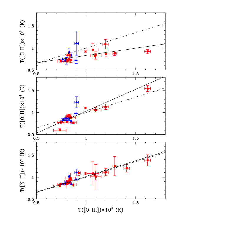
Figure 2: Correlations between various $T_{\rm e}$ diagnostics. Filled (red) squares show our measurements for extragalactic H II regions and those of NGC 5253 from López-Sánchez et al. (2007), 30 Doradus from Peimbert (2003), and NGC 5471 from Esteban et al. (2002). Filled (blue) triangles show measurements for a sample of Galactic H II regions taken from the compilation by García-Rojas & Esteban (2007). The solid lines represent the least-squares fit of the measurements. The dashed lines show the predicted correlations from Garnett (1992) based on photoionization models.

The data compiled in Table 5 provides a relatively large number of different $T_{\rm e}$ determinations, in particular those associated with low ionization potential ions: [N II], [O II], and [S II]. This allows us to compare the consistency of different temperature scales. Garnett (1992) constructed photoionization models that provide simple scaling relations between temperatures measured from different ions. This author obtains the following relation between $T_{\rm e}$([O III]) and other temperature indicators of low ionization degree ions –such as $T_{\rm e}$([N II]), $T_{\rm e}$([O II]), and $T_{\rm e}$([S II])– valid for the temperature range from 2000 to 18,000 K:

$$T_{e}([{\rm N\medspace II}])=T_{e}([{\rm O\medspace II}])=T_{e}([{\rm S\medspace II}])=0.70\times T_{e}([{\rm O\medspace III}])+3000~{}{\rm K}.$$ (2)

Similar relationships between $T_{\rm e}$([O III]) and $T_{\rm e}$([O II]) have been obtained by other authors (Campbell et al., 1986; Izotov et al., 1994; Pilyugin et al., 2006) and have been extensively used in many works. Several authors have tried to make observational tests of the reliability of these relations (Garnett et al., 1997; Kennicutt et al., 2003; Pérez-Montero & Díaz, 2003; Hägele et al., 2006, 2008; Bresolin et al., 2009). The $T_{\rm e}$([N II]) vs. $T_{\rm e}$([O III]) relationship has been the most difficult one to test because of the paucity of good determinations of the $T_{\rm e}$([N II]) temperature indicator. This is because most studies have focused on the determination of chemical abundances in low-metallicity, high-excitation EHRs, especially H II galaxies, where the [N II] $\lambda$ 5755 line is very faint (Pérez-Montero & Díaz, 2003; Hägele et al., 2006, 2008). Kennicutt et al. (2003) studied H II regions in M 101, a group of objects whose properties are more similar to those of most of our EHRs, but the small number of objects with $T_{\rm e}$([N II]) determinations in their sample does not permit to obtain a clear trend between $T_{\rm e}$([N II]) and $T_{\rm e}$([O III]), indicating that more data were needed to draw meaningful conclusions. In Figure 2, we show the relations between $T_{\rm e}$([N II]), $T_{\rm e}$([O II]), and $T_{\rm e}$([S II]) with respect to $T_{\rm e}$([O III]) obtained from the data presented in this paper and those of NGC 5253 (López-Sánchez et al., 2007), 30 Doradus (Peimbert, 2003), NGC 5471 (Esteban et al., 2002), and the compilation of data for a sample of Galactic H II regions of García-Rojas & Esteban (2007). These data have been included because they are also based on high-spatial resolution spectroscopy (except in the cases of NGC 5447 and NGC 5471, where intermediate-resolution spectroscopy was used) and they have been analyzed in the same manner as the present sample, using the same atomic dataset and considering the recombination contribution to both the [N II] and [O II] line intensities. In the figure, we can see a rather clear linear relation between $T_{\rm e}$([N II]) with respect to $T_{\rm e}$([O III]), which is a susbtantial improvement with respect to the previous results by Kennicutt et al. (2003). Our least-squares fit to the points –weighted by their observational errors– of the $T_{\rm e}$([N II]) vs. $T_{\rm e}$([O III]) diagram gives:

$$T_{e}([{\rm N\medspace II}])=0.71\times T_{e}([{\rm O\medspace III}])+3050~{}{\rm K},$$ (3)

with a correlation coefficient of 0.91. It is remarkable that this empirical relation is almost identical to the theoretically predicted relationship from Garnett (1992), confirming that the use of Garnett’s relation between these two indicators is entirely reliable (the same conclusion has been drawn by Bresolin et al. 2009). This is a result of special interest because while $T_{\rm e}$([O III]) usually cannot be derived in metal-rich H II regions –where the [O III] $\lambda$4363 auroral line becomes very faint– $T_{\rm e}$([N II]) can be more easily determined from optical spectra (see Bresolin, 2006), and shows a very weak dependence on $n_{\rm e}$.

The apparent lack of consistency between $T_{\rm e}$([O II]) and $T_{\rm e}$([O III]) found by all the authors that have studied the empirical relation of these temperature indicators (Kennicutt et al., 2003; Pérez-Montero & Díaz, 2003; Hägele et al., 2006, 2008) is remarkable. Kennicutt et al. (2003) proposed several possible sources of such inconsistency: a) the recombination contribution to [O II] line intensity, b) the large contribution of collisional de-excitation to the [O II] line ratios –dependence on $n_{\rm e}$– used for deriving $T_{\rm e}$([O II]), which is more important than for the rest of the indicators, except $T_{\rm e}$([S II]), c) radiative transfer effects, d) observational uncertainties in the interstellar reddening, e) contamination by OH airglow emission of the [O II] multiplet around 7325 Å. Pérez-Montero & Díaz (2003) and Hägele et al. (2006, 2008) obtain also a large scatter in their $T_{\rm e}$([O II]) vs. $T_{\rm e}$([O III]) diagrams, that include a large number of data points from the literature. These authors indicate that the scatter is probably due to the dependence of $T_{\rm e}$([O II]) on electron density. However, our results shown in Figure 2 indicate a tighter and rather linear relation between $T_{\rm e}$([O II]) and $T_{\rm e}$([O III]). The least-squares fit gives:

$$T_{e}([{\rm O\medspace II}])=0.99\times T_{e}([{\rm O\medspace III}])+410~{}{\rm K},$$ (4)

with a correlation coefficient of 0.88, indicating that the use of Garnett’s relationship between $T_{\rm e}$([O II]) and $T_{\rm e}$([O III]) seems to be a reasonable approximation. It is important to remark that our data have been corrected for the recombination contribution to [O II] –as also done by Pérez-Montero & Díaz (2003); Hägele et al. (2006, 2008)– and that the use of high spectral-resolution spectra precludes the contamination by OH airglow emission of the red [O II] lines. The comparison of our result with the previous ones from the literature is puzzling. Considering that most of the scatter shown in the $T_{\rm e}$([O II]) vs. $T_{\rm e}$([O III]) diagrams of Pérez-Montero & Díaz (2003) and Hägele et al. (2006, 2008) should be due to the inclusion of inhomogeneous data points from the literature, we think that the sensitivity of $T_{\rm e}$([O II]) to many different factors makes the statistical use of this indicator ill-advised when using inhomogeneous datasets.

As it can be seen in Figure 2, the third relationship studied: $T_{\rm e}$([S II]) vs. $T_{\rm e}$([O III]) shows a somewhat different behaviour than the previous ones. The data points show a larger scatter and the least-squares fit gives:

$$T_{e}([{\rm S\medspace II}])=0.33\times T_{e}([{\rm O\medspace III}])+5015~{}{\rm K},$$ (5)

with a correlation coefficient of 0.53, lower than in the previous cases. A large scatter in this relation is also evident in the data obtained by Pérez-Montero & Díaz (2003) and Hägele et al. (2008). A common result of these works is that $T_{\rm e}$([S II]) is smaller than $T_{\rm e}$([O II]) in most cases, in agreement with our results. There are several arguments to explain this behavior: a) due to the lower ionization potential of neutral sulphur, the zone of S⁺ should not coincide with the zone where N⁺ and O⁺ are present –which are essentially cospatial– and this may be reflected in somewhat different temperatures in both zones, b) the contribution of [S II] emission from diffuse ionized gas due to photon leakage from the H II region, c) the dependence of $T_{\rm e}$([S II]) on electron density, d) some recombination contribution to [S II] line intensities.

Table 6: Ionic and Total Abundances

	NGC 595		NGC 604		H1013		NGC 5461		NGC 5447
	$t^{2}$ = 0.000	$t^{2}$ = 0.036	$t^{2}$ = 0.000	$t^{2}$ = 0.034	$t^{2}$ = 0.000	$t^{2}$ = 0.037	$t^{2}$ = 0.000	$t^{2}$ = 0.014	$t^{2}$ = 0.000	$t^{2}$ = 0.032
Ionic Abundances from Collisionally Excited Lines
N+	7.13$\pm$0.02	7.28$\pm$0.06	6.82$\pm$0.03	6.94$\pm$0.04	7.35$\pm$0.04	7.52$\pm$0.11	6.85$\pm$0.04	6.89$\pm$0.06	6.43$\pm$0.05	6.51$\pm$0.05
O+	8.27$\pm$0.03	8.44$\pm$0.06	7.92$\pm$0.04	8.06$\pm$0.05	8.23$\pm$0.06	8.43$\pm$0.13	7.80$\pm$0.06	7.85$\pm$0.08	7.57$\pm$0.11	7.66$\pm$0.11
O++	7.99$\pm$0.06	8.33$\pm$0.07	8.19$\pm$0.03	8.45$\pm$0.04	8.06$\pm$0.12	8.42$\pm$0.12	8.29$\pm$0.03	8.38$\pm$0.07	8.27$\pm$0.02	8.46$\pm$0.06
Ne++	6.73$\pm$0.08	7.11$\pm$0.16	7.27$\pm$0.03	7.56$\pm$0.08	7.01$\pm$0.16	7.41$\pm$0.36	7.46$\pm$0.04	7.56$\pm$0.11	$\cdots$	$\cdots$
S+	5.50$\pm$0.02	5.65$\pm$0.06	5.47$\pm$0.03	5.59$\pm$0.04	5.63$\pm$0.04	5.80$\pm$0.11	5.34$\pm$0.04	5.38$\pm$0.06	5.23$\pm$0.05	5.31$\pm$0.05
S++	$\cdots$	$\cdots$	$\cdots$	$\cdots$	6.88$\pm$0.23	7.29$\pm$0.40	6.76$\pm$0.06	6.86$\pm$0.12	6.58$\pm$0.06	6.79$\pm$0.12
Cl++	4.80$\pm$0.06	5.12$\pm$0.13	4.58$\pm$0.03	4.83$\pm$0.07	4.72$\pm$0.12	5.07$\pm$0.27	4.59$\pm$0.04	4.68$\pm$0.10	4.55$\pm$0.04	4.73$\pm$0.09
Ar++	6.14$\pm$0.06	6.42$\pm$0.12	6.04$\pm$0.03	6.26$\pm$0.06	6.15$\pm$0.12	6.45$\pm$0.23	6.09$\pm$0.05	6.16$\pm$0.09	6.02$\pm$0.04	6.18$\pm$0.08
Ar3+	$\cdots$	$\cdots$	$\cdots$	$\cdots$	$\cdots$	$\cdots$	4.20$\pm$0.10	4.29$\pm$0.14	4.26$\pm$0.05	4.45$\pm$0.10
Fe++	5.18$\pm$0.17	5.34$\pm$0.18	5.34$\pm$0.09	5.48$\pm$0.09	5.55$\pm$0.18	5.73$\pm$0.19	5.55$\pm$0.18	5.60$\pm$0.18	5.38$\pm$0.29	5.47$\pm$0.30
Ionic Abundances from Recombination Lines
He+	10.834$\pm$0.004	10.830$\pm$0.04	10.869$\pm$0.005	10.866$\pm$0.005	10.86$\pm$0.01	10.86$\pm$0.01	10.86$\pm$0.01	10.86$\pm$0.01	10.90$\pm$0.02	10.88$\pm$0.02
He++	$\cdots$		$\cdots$		$\cdots$		7.80$\pm$0.11		$\cdots$
C++	8.07$\pm$0.12		8.19$\pm$0.11		8.40$\pm$0.12		8.13$\pm$0.20		8.06$\pm$0.11
O++	8.33$\pm$0.07		8.45$\pm$0.04		8.42$\pm$0.11		8.38$\pm$0.07		8.46$\pm$0.07
Total Abundances
He	10.849$\pm$0.004	10.845$\pm$0.004	10.887$\pm$0.005	10.884$\pm$0.005	10.87$\pm$0.01	10.87$\pm$0.01	10.88$\pm$0.01	10.88$\pm$0.01	10.90$\pm$0.02	10.88$\pm$0.02
C	8.53$\pm$0.12		8.40$\pm$0.11		8.67$\pm$0.12		8.30$\pm$0.20		8.20$\pm$0.12
N	7.31$\pm$0.05	7.53$\pm$0.10	7.28$\pm$0.05	7.49$\pm$0.07	7.57$\pm$0.10	7.82$\pm$0.19	7.46$\pm$0.08	7.54$\pm$0.11	7.21$\pm$0.12	7.38$\pm$0.13
O	8.45$\pm$0.03	8.69$\pm$0.05	8.38$\pm$0.02	8.60$\pm$0.03	8.45$\pm$0.06	8.73$\pm$0.09	8.41$\pm$0.03	8.49$\pm$0.06	8.35$\pm$0.02	8.52$\pm$0.06
Ne	7.19$\pm$0.10	7.47$\pm$0.19	7.46$\pm$0.05	7.70$\pm$0.10	7.41$\pm$0.21	7.72$\pm$0.42	7.59$\pm$0.06	7.67$\pm$0.15	$\cdots$	$\cdots$
S	$\cdots$	$\cdots$	$\cdots$	$\cdots$	6.91$\pm$0.23	7.31$\pm$0.48	6.86$\pm$0.06	6.93$\pm$0.12	6.72$\pm$0.06	6.88$\pm$0.12
Ar	6.38$\pm$0.08	6.60$\pm$0.13	6.22$\pm$0.03	6.47$\pm$0.07	6.35$\pm$0.14	6.62$\pm$0.24	6.12$\pm$0.05	6.19$\pm$0.09	6.04$\pm$0.04	6.20$\pm$0.08
Fe	5.34$\pm$0.19	5.55$\pm$0.21	5.73$\pm$0.10	5.94$\pm$0.11	5.74$\pm$0.23	5.98$\pm$0.26	6.08$\pm$0.20	6.15$\pm$0.21	6.06$\pm$0.33	6.23$\pm$0.35

Table 7: Ionic and Total Abundances

	VS 24	VS 38	VS 44		NGC 2363		K932
	$t^{2}$ = 0.000	$t^{2}$ = 0.000	$t^{2}$ = 0.000	$t^{2}$ = 0.039	$t^{2}$ = 0.000	$t^{2}$ = 0.120	$t^{2}$ = 0.000	$t^{2}$ = 0.033
Ionic Abundances from Collisionally Excited Lines
N+	7.07$\pm$0.04	6.97$\pm$0.05	6.90$\pm$0.03	7.04$\pm$0.05	5.20$\pm$0.06	5.43$\pm$0.07	6.85$\pm$0.02	6.96$\pm$0.03
O+	8.09$\pm$0.05	8.03$\pm$0.08	7.97$\pm$0.04	8.13$\pm$0.05	6.53$\pm$0.09	6.77$\pm$0.05	7.83$\pm$0.03	7.95$\pm$0.04
O++	8.05$\pm$0.06	7.93$\pm$0.04	8.13$\pm$0.03	8.43$\pm$0.06	7.73$\pm$0.02	8.02$\pm$0.05	8.28$\pm$0.02	8.52$\pm$0.04
Ne++	6.93$\pm$0.09	6.93$\pm$0.06	7.16$\pm$0.04	7.49$\pm$0.11	6.92$\pm$0.02	7.23$\pm$0.07	7.51$\pm$0.03	7.77$\pm$0.07
S+	5.52$\pm$0.04	5.55$\pm$0.05	5.49$\pm$0.03	5.63$\pm$0.05	4.34$\pm$0.06	4.56$\pm$0.07	5.28$\pm$0.02	5.39$\pm$0.03
S++	6.73$\pm$0.12	6.37$\pm$0.09	6.73$\pm$0.06	7.07$\pm$0.11	5.70$\pm$0.03	6.01$\pm$0.08	6.76$\pm$0.04	7.03$\pm$0.07
Cl++	4.58$\pm$0.07	4.25$\pm$0.07	4.54$\pm$0.04	4.83$\pm$0.09	3.59$\pm$0.02	3.87$\pm$0.07	4.61$\pm$0.03	4.84$\pm$0.06
Cl3+	$\cdots$	$\cdots$	$\cdots$	$\cdots$	3.84$\pm$0.18	4.12$\pm$0.14	$\cdots$	$\cdots$
Ar++	5.97$\pm$0.06	5.88$\pm$0.05	6.00$\pm$0.04	6.25$\pm$0.08	5.19$\pm$0.03	5.44$\pm$0.06	6.10$\pm$0.03	6.30$\pm$0.05
Ar3+	$\cdots$	$\cdots$	$\cdots$	$\cdots$	4.73$\pm$0.02	5.03$\pm$0.07	3.89$\pm$0.08	4.14$\pm$0.08
Fe++	5.47$\pm$0.17	5.36$\pm$0.31	5.56$\pm$0.09	5.72$\pm$0.09	4.36$\pm$0.23	4.58$\pm$0.21	5.21$\pm$0.07	5.32$\pm$0.07
Fe3+	$\cdots$	$\cdots$	$\cdots$	$\cdots$	5.02$\pm$0.21	5.23$\pm$0.22	$\cdots$	$\cdots$
Ionic Abundances from Recombination Lines
He+	10.820$\pm$0.007	10.881$\pm$0.006	10.848$\pm$0.006	10.833$\pm$0.006	10.88$\pm$0.01	10.85$\pm$0.01	10.911$\pm$0.005	10.907$\pm$0.005
He++	$\cdots$	$\cdots$	$\cdots$		8.34$\pm$0.02		$\cdots$
C++	8.15$\pm$0.24	8.27$\pm$0.15	7.98$\pm$0.18		7.55$\pm$0.09		8.31$\pm$0.13
O++	$<$8.50	$<$8.54	8.43$\pm$0.06		8.02$\pm$0.05		8.52$\pm$0.04
Total Abundances
He	10.841$\pm$0.007	10.902$\pm$0.006	10.863$\pm$0.006	10.848$\pm$0.006	10.88$\pm$0.01	10.85$\pm$0.01	10.920$\pm$0.005	10.916$\pm$0.005
C	8.46$\pm$0.24	8.50$\pm$0.15	8.32$\pm$0.18		7.75$\pm$0.09		8.46$\pm$0.13
N	7.35$\pm$0.07	7.23$\pm$0.11	7.29$\pm$0.05	7.52$\pm$0.08	6.43$\pm$0.07	6.70$\pm$0.10	7.44$\pm$0.04	7.63$\pm$0.06
O	8.37$\pm$0.04	8.29$\pm$0.05	8.36$\pm$0.02	8.61$\pm$0.04	7.76$\pm$0.02	8.04$\pm$0.05	8.41$\pm$0.02	8.62$\pm$0.03
Ne	7.25$\pm$0.11	7.29$\pm$0.09	7.39$\pm$0.06	7.67$\pm$0.13	6.95$\pm$0.03	7.25$\pm$0.10	7.64$\pm$0.04	7.88$\pm$0.09
S	6.77$\pm$0.11	6.45$\pm$0.08	6.79$\pm$0.06	7.12$\pm$0.11	5.98$\pm$0.03	6.28$\pm$0.07	6.85$\pm$0.04	7.12$\pm$0.07
Ar	6.14$\pm$0.06	6.06$\pm$0.07	6.16$\pm$0.04	6.44$\pm$0.08	5.32$\pm$0.02	5.58$\pm$0.05	6.13$\pm$0.04	6.32$\pm$0.05
Fe	5.71$\pm$0.19	5.58$\pm$0.35	5.89$\pm$0.10	6.13$\pm$0.12	5.44$\pm$0.24	5.71$\pm$0.23	5.71$\pm$0.08	5.90$\pm$0.09

4.2 Ionic Abundances from CELs and RLs

Ionic abundances of N⁺, O⁺, O⁺⁺, Ne⁺⁺, S⁺, S⁺⁺, Cl⁺⁺, Cl³⁺, Ar⁺⁺, and Ar³⁺ have been derived from CELs by making use of the IRAF task ionic of the package NEBULAR. We have assumed a two-zone scheme adopting $T_{\rm e}$([N II]) for ions with a low ionization potential (N⁺, O⁺, and S⁺) and $T_{\rm e}$([O III]) for ions with a high ionization potential (O⁺⁺, Ne⁺⁺, S⁺⁺ Cl⁺⁺, Cl³⁺, Ar⁺⁺, and Ar³⁺). All the ionic abundances are included in Tables 6–8. We have used neither $T_{\rm e}$([O II]) nor $T_{\rm e}$([S II]) for the abundance determinations. As discussed in §§ 4.1, the $T_{\rm e}$([O II]) may be affected by several sources of uncertainty and, in principle, may be a less confident temperature indicator. On the other hand, as we pointed out in §§ 4.1, $T_{\rm e}$([S II]) is somewhat lower than $T_{\rm e}$([N II]) or $T_{\rm e}$([O II]) in most of the objects. This effect has been reported previously in several Galactic H II regions (García-Rojas et al., 2005, 2006, 2007), and might be produced by the presence of a temperature stratification in the outer zones of the nebulae or, conversely, by uncertainties in the atomic parameters of the ion. The H II region at the center of M 83 is the only object without a direct determination of $T_{\rm e}$([O III]). For the abundance determinations adopted for this nebula we have assumed $T_{\rm e}$([O III]) = $T_{\rm e}$([N II]). The use of either the theoretical or the empirical relationships between $T_{\rm e}$([O III]) and $T_{\rm e}$([N II]) shown in equations 2 or 3 provides a value of $T_{\rm e}$([O III]) of about 2900 K, which gives unreasonably high abundances, for example 12+log(O⁺⁺/H⁺) = 9.72 or even 12+log(Ne⁺⁺/H⁺) = 10.22. As it has been demostrated by Stasińska (1978, 2005), high-metallicity –and low-temperature– H II regions may have large temperature gradients that could produce differences between the electron temperatures determined from line intensity ratios and the mean ionic temperatures (those obtained from photoionization models and used to derive the equations obtained by Garnett, 1992). This effect can naturally explain the inappropriateness of the $T_{\rm e}$([O III]) estimated for the H II region at the center of M 83.

The errors in the ionic abundances shown in tables 6–8 have been computed as the quadratic sum of the independent contributions of $n_{\rm e}$, $T_{\rm e}$, and line flux uncertainties. We have considered two sets of abundances, one for $t^{\rm 2}$ = 0 and one for $t^{\rm 2}$ $>$ 0 (see §§ 5.1).

[Fe II] lines have been detected in the spectra of some of our sample objects. Unfortunately, these lines are severely affected by continuum fluorescence effects (see Rodríguez, 1999; Verner et al., 2000) and are not suitable for abundance determinations. [Fe III] lines have been detected in all the objects except at the nucleus of M83. For the calculations of the Fe⁺⁺/H⁺ ratio, we have used a 34-level model atom that uses collision strengths from Zhang (1996) and the transition probabilities of Quinet (1996) as well as the new transitions found by Johansson et al. (2000). The adopted values of the Fe⁺⁺/H⁺ abundance correspond to the mean of the abundances obtained for the different [Fe III] lines measured for each object. Several [Fe IV] lines have been detected in NGC 2363. The Fe³⁺/H⁺ ratio has been derived using a 33-level model atom where all collision strengths are those calculated by Zhang & Pradhan (1997) and the transition probabilities are those recommended by Froese Fischer et al. (2008).

We have measured several He I emission lines in the spectra of the sample objects. These lines arise mainly from recombination, but they can be affected by collisional excitation and self-absorption effects. We have used the effective recombination coefficients of Storey & Hummer (1995) for H I and those computed by Porter et al. (2005), with the interpolation formulae provided by Porter et al. (2007) for He I. The collisional contribution was estimated from Sawey & Berrington (1993) and Kingdon & Ferland (1995), and the optical depth in the triplet lines were derived from the computations by Benjamin et al. (2002). We have not corrected the He I lines for underlying stellar absorption because: (a) the use of high-spectral resolution data; (b) the lack of appropriate determinations of He I EWs in absorption for OB associations and for all the brightest He I lines along the optical spectrum (see Kennicutt et al., 2003). We have determined the He⁺/H⁺ ratio for for $t^{\rm 2}$ = 0 and $t^{\rm 2}$ $>$ 0 from a maximum likelihood method (Peimbert et al., 2000, 2002). The He II $\lambda$4686 line has been detected in three objects: NGC 5461, NGC 2363, and NGC 4861. We have determined the He⁺⁺/H⁺ ratio using the line emissivities calculated by Hummer & Storey (1987) and Storey & Hummer (1995). We have not calculated the He⁺⁺/H⁺ ratios for $t^{\rm 2}$ $>$ 0 considering the small effect of temperature fluctuations on this abundance and the negligible contribution of this ion to the total He/H ratio.

The high signal-to-noise of the spectra has permitted to detect and measure pure RLs of O II and C II in many of the sample objects. These lines have almost the same $T_{\rm e}$ and $n_{\rm e}$ dependence as H I lines. This almost eliminates the bias in the derived abundances in the case of line-of-sight temperature variations, with respect to abundances derived from CELs.

Let $I$($\lambda$) be the intensity of a RL of an element X, $i$ times ionized, at wavelength $\lambda$; then the abundance of the ionization state $i+1$ of element X is given by

$$\frac{N({\rm X}^{i+1})}{N({\rm H}^{+})}=\frac{\lambda({\rm\AA})}{4861}\frac{\alpha_{eff}({\rm H}\beta)}{\alpha_{eff}(\lambda)}\frac{I(\lambda)}{I({\rm H}\beta)},$$ (6)

where $\alpha_{eff}(\lambda)$ and $\alpha_{eff}({\rm H}\beta)$ are the effective recombination coefficients for the line and for H$\beta$, respectively. The $\alpha_{eff}({\rm H}\beta)/\alpha_{eff}(\lambda)$ ratio is almost independent of the adopted temperatures and densities.

Following Esteban et al. (1998), we have determined the O⁺⁺ abundances from the estimated total intensity of the RLs of multiplet 1 of O II. This last quantity is obtained by multiplying the sum of the intensities of the individual lines of multiplet 1 of O II observed in a given object by the multiplet correction factor, defined as:

$$m_{cf}=\frac{\sum_{all}s_{ij}}{\sum_{obs}s_{ij}},$$ (7)

where $s_{ij}$ are the theoretical line strengths, which are constructed assuming that they are proportional to the populations of their parent levels, if we assume LTE computations predictions. The upper sum runs over $all$ the lines of the multiplet, and the lower sum runs over the $observed$ lines of the multiplet. The lines of multiplet 1 of O II are not in LTE for densities $n_{\rm e}$ $<$ 10,000 cm^-3 (Ruiz et al., 2003; Tsamis et al., 2003). We have used the prescriptions given by Peimbert et al. (2005) to calculate the appropriate corrections for the relative strengths between the individual lines of multiplet 1. The O⁺⁺ and C⁺⁺ abundances from RLs have been calculated using the representative $T_{\rm e}$-values of these ions, $T_{\rm e}$([O III]), and the effective recombination coefficients that are available in the literature (Storey 1994 for O II assuming LS coupling, and Davey et al. 2000 for C II). In the case of those objects where only upper limits of the O II $\lambda$4549 intensity have been estimated, the corresponding upper limit of the O⁺⁺ abundance has been derived from the intensity of that line and the prescription given by Peimbert et al. (2005) for O II $\lambda$4549.

4.3 Total Abundances

To derive the total gas-phase abundances of the different elements present in our spectra, we have to correct for the unseen ionization stages by using a set of ionization correction factors (ICFs). The total helium abundance has been corrected for the presence of neutral helium using the ionization fractions obtained from the photoionization models of Stasińska (1990) that reproduce the O abundance, O⁺⁺/O⁺ ratio, $T_{\rm e}$([O III]), and $T_{\rm e}$([N II]) measured in each object. In the case of M83, we have not determined the total He abundance due to the low ionization degree of the nebula, that implies a large contribution of neutral helium and a very uncertain ICF. In the cases of NGC 5461, NGC 2363, and NGC 4861 –whose spectra show a rather faint He II $\lambda$4686 line– we have assumed that the total He/H ratio is just the sum of He⁺/H⁺ and a small contribution of He⁺⁺/H⁺, i.e. the amount of neutral helium is negligible inside these nebulae.

For C we have adopted an ICF-value for the presence of C⁺ obtained from the photoionization models by Garnett et al. (1999). This correction seems to be fairly appropriate considering the relatively high ionization degree of the objects where the C II $\lambda$4267 line has been detected. In order to derive the total abundance of nitrogen we have used the usual ICF based on the similarity between the ionization potential of N⁺ and O⁺ (Peimbert & Costero, 1969) in all the cases. Due to the absence of the He II $\lambda$ 4686 line in most of the objects, the total abundance of oxygen has been calculated as the sum of O⁺ and O⁺⁺ abundances. We decided to make the same approximation in the cases of NGC 5461, NGC 2363, and NGC 4861 due to the weakness of the He II $\lambda$4686 line detected in these objects, which implies an irrelevant contribution of O³⁺.

The only measurable CELs of Ne in the optical range are those of Ne²⁺ but the fraction of Ne⁺ may be important in the nebula. For this element, we have adopted the usual expression proposed by Peimbert & Costero (1969) that assumes that the ionization structure of Ne is similar to that of O. We have measured CELs of two ionization stages of S: S⁺ and S²⁺, and used the ICF proposed by Stasińska (1978) –which is based on photoionization models of H II regions– to take into account the presence of S³⁺. For argon we have determinations of the Ar²⁺ abundance for all the objects and also of the Ar³⁺ abundance for NGC 5461, NGC 5447, NGC 2363, K932, and NGC 4861. However, some contribution of Ar⁺ is expected. We have adopted the ICF recommended by Izotov et al. (1994) for this element.

Finally, for iron, we have determined the Fe⁺⁺ abundance for all the objects and also the Fe³⁺ abundance for NGC 2363. Some small contribution of Fe⁺ should be present, mainly in the nebulae of lower ionization degree. We have used an ICF scheme based on photoionization models of Rodríguez & Rubin (2005) to obtain the total Fe/H ratio using the Fe⁺⁺ abundances.

In Tables 6–8 we show the total abundances for $t^{\rm 2}$ = 0 and for the $t^{\rm 2}$-value adopted in those objects where this parameter was estimated (see §§ 5.1).

Table 8: Ionic and Total Abundances

	NGC 1741	NGC 4395-70	NGC 4861	M 83
Ionic Abundances from Collisionally Excited Lines
N+	6.72$\pm$0.09	6.35$\pm$0.26	5.70$\pm$0.13	8.48$\pm$0.09
O+	7.77$\pm$0.14	7.53$\pm$0.24	7.19$\pm$0.24	8.94$\pm$0.09
O++	8.30$\pm$0.07	7.95$\pm$0.06	7.98$\pm$0.02	7.79$\pm$0.12
Ne++	7.53$\pm$0.10	7.24$\pm$0.07	7.24$\pm$0.02	7.76$\pm$0.24
S+	5.64$\pm$0.08	5.59$\pm$0.22	4.89$\pm$0.12	6.76$\pm$0.08
S++	6.75$\pm$0.14	6.38$\pm$0.11	6.23$\pm$0.03	6.76$\pm$0.08
Cl++	$\cdots$	4.32$\pm$0.11	4.07$\pm$0.04	$\cdots$
Ar++	5.98$\pm$0.08	5.76$\pm$0.06	5.60$\pm$0.02	6.10$\pm$0.12
Ar3+	$\cdots$	$\cdots$	4.55$\pm$0.02	$\cdots$
Fe++	5.68$\pm$0.19	5.70$\pm$0.30	5.18$\pm$0.21	$\cdots$
Ionic Abundances from Recombination Lines
He+	10.72$\pm$0.02	10.82$\pm$0.02	10.90$\pm$0.01	10.58$\pm$0.02
He++	$\cdots$	$\cdots$	8.73$\pm$0.03	$\cdots$
C++	$<$7.97	$<$7.47	$<$7.49	$\cdots$
O++	$<$8.68	$<$8.72	$<$8.25	$\cdots$
Total Abundances
He	10.73$\pm$0.02	10.83$\pm$0.02	10.91$\pm$0.01	$\cdots$
N	7.36$\pm$0.18	6.56$\pm$0.28	6.56$\pm$0.28	8.51$\pm$0.15
O	8.41$\pm$0.06	8.09$\pm$0.15	8.05$\pm$0.04	8.97$\pm$0.08
Ne	7.64$\pm$0.14	7.38$\pm$0.17	7.30$\pm$0.04	8.94$\pm$0.30
S	6.89$\pm$0.13	6.51$\pm$0.10	6.40$\pm$0.03	7.42$\pm$0.23
Ar	6.23$\pm$0.11	5.98$\pm$0.23	5.65$\pm$0.02	$\cdots$
Fe	5.95$\pm$0.25	5.97$\pm$0.42	5.45$\pm$0.33	$\cdots$

Table 9: Comparison of Ionic Abundances and $t^{\rm 2}$ Parameter

	O++/H+				C++/H+
Object	CELs	RLs	ADF(O++)	$t^{\rm 2}$(O++)	CELs	RLs	ADF(C++)	$t^{\rm 2}$(C++)	$t^{\rm 2}$(He+)
NGC 595	7.99$\pm$0.06	8.33$\pm$0.07	0.34$\pm$0.08	0.036$\pm$0.012	$\cdots$	8.07$\pm$0.12	$\cdots$	$\cdots$	0.033$\pm$0.009
NGC 604	8.19$\pm$0.02	8.45$\pm$0.04	0.26$\pm$0.04	0.034$\pm$0.008	$\cdots$	8.19$\pm$0.11	$\cdots$	$\cdots$	0.022$\pm$0.010
H1013	8.06$\pm$0.12	8.42$\pm$0.11	0.36$\pm$0.13	0.037$\pm$0.020	$\cdots$	8.40$\pm$0.12	$\cdots$	$\cdots$	0.031$\pm$0.017
NGC 5461	8.29$\pm$0.03	8.38$\pm$0.07	0.09$\pm$0.08	0.014$\pm$0.014	8.27/7.90	8.13$\pm$0.20	$-$0.14/0.23	$<$0/0.028	0.057$\pm$0.018
NGC 5447	8.27$\pm$0.02	8.46$\pm$0.07	0.19$\pm$0.07	0.032$\pm$0.007	$\cdots$	8.06$\pm$0.11	$\cdots$	$\cdots$	0.094$\pm$0.034
VS 24	8.05$\pm$0.06	$<$8.50	$<$0.45	$\cdots$	$\cdots$	8.15$\pm$0.24	$\cdots$	$\cdots$	0.075$\pm$0.012
VS 38	7.93$\pm$0.04	$<$8.54	$<$0.61	$\cdots$	8.00/7.84	8.27$\pm$0.15	0.27/0.43	0.026/0.035	0.057$\pm$0.015
VS 44	8.13$\pm$0.03	8.43$\pm$0.06	0.30$\pm$0.06	0.039$\pm$0.010	8.08/7.85	7.98$\pm$0.18	$-$0.10/0.13	$<$0/0.018	0.066$\pm$0.010
NGC 2363	7.73$\pm$0.02	8.02$\pm$0.05	0.29$\pm$0.05	0.120$\pm$0.022	7.15	7.55$\pm$0.09	0.40	0.153	0.101$\pm$0.019
K932	8.28$\pm$0.02	8.52$\pm$0.04	0.24$\pm$0.04	0.033$\pm$0.007	$\cdots$	8.31$\pm$0.13	$\cdots$	$\cdots$	0.030$\pm$0.009
NGC 1741	8.30$\pm$0.07	$<$8.68	$<$0.38	$\cdots$	$\cdots$	$<$7.97	$\cdots$	$\cdots$	0.035$\pm$0.076
NGC 4395-70	7.95$\pm$0.06	$<$8.72	$<$0.77	$\cdots$	$\cdots$	$<$7.47	$\cdots$	$\cdots$	0.125$\pm$0.064
NGC 4861	7.98$\pm$0.02	$<$8.25	$<$0.27	$\cdots$	7.44$\pm$0.11	$<$7.49	$<$0.05	$\cdots$	0.103$\pm$0.020
M 83	7.79$\pm$0.12	$\cdots$	$\cdots$	$\cdots$	$\cdots$	$\cdots$	$\cdots$	$\cdots$	0.036$\pm$0.010

5 Discussion

5.1 The Abundance Discrepancy Factor in the Sample Objects

Table 10: Abundance Gradients in M33, M101, NGC 2403, and the Milky Way

Galaxy	O/H (CELs)	O/H (RLs)	C/H	C/O (RLs)
With respect to RG
M 33	$-$0.056 $\pm$ 0.029	$-$0.072 $\pm$ 0.047	$-$0.105 $\pm$ 0.120	-0.033 $\pm$ 0.130
M 101	$-$0.022 $\pm$ 0.004	$-$0.017 $\pm$ 0.009	$-$0.046 $\pm$ 0.012	-0.029 $\pm$ 0.020
NGC 2403	$+$0.012 $\pm$ 0.021	$\cdots$	$-$0.097 $\pm$ 0.127	$\cdots$
Milky Way	$-$0.040 $\pm$ 0.006	$-$0.044 $\pm$ 0.010	$-$0.103 $\pm$ 0.018	-0.059 $\pm$ 0.020
With respect to R0
M 33	$-$0.39 $\pm$ 0.20	$-$0.50 $\pm$ 0.32	$-$0.72 $\pm$ 0.83	-0.22 $\pm$ 0.98
M 101	$-$0.62 $\pm$ 0.10	$-$0.50 $\pm$ 0.25	$-$1.32 $\pm$ 0.33	-0.65 $\pm$ 0.49
NGC 2403	$+$0.09 $\pm$ 0.17	$\cdots$	$-$0.77 $\pm$ 1.00	$\cdots$

In Table 9, we include the O⁺⁺ and C⁺⁺ abundances determined from RLs and CELs for the sample objects as well as the ADF for each ion. The C⁺⁺ abundance determinations based on CELs included in the table have been calculated from the intensities of [C III] $\lambda$1907 + C III] $\lambda$1909 lines, which are in the UV and come from the literature (Garnett et al., 1995, 1999; Kobulnicky & Skillman, 1998). Except in the cases of NGC 2363 and NGC 4861, the rest of the C⁺⁺/H⁺ ratios based on CELs have two possible values, which correspond to the higher and lower limits adopted by Garnett et al. (1999) because of the uncertainty in the choice of the UV reddening function from their data. Garnett et al. (1995) determined the C⁺⁺ abundance of NGC 2363 from UV CELs, and because of its low reddening, the uncertainty in the UV reddening function is not a concern for this object. In the case of NGC 4861, the choice of the UV reddening law can also affect but not very importantly because its relatively low extinction (see Kobulnicky & Skillman, 1998).

As it can be seen in Table 9, the values of the ADF(O⁺⁺) are remarkably similar in all the objects, with a mean value of 0.26 $\pm$ 0.09 dex, which is very similar to the mean ADF(O⁺⁺) obtained for a sample of Galactic H II regions (see García-Rojas & Esteban, 2007, and references therein) and for other EHRs (0.30 $\pm$ 0.09 dex, see López-Sánchez et al., 2007, and references therein). The upper limits of the ADF(O⁺⁺) included in Table 9 are always of the order or larger than the mean ADF(O⁺⁺). In the case of the ADF(C⁺⁺) the results are not so clear because of the limited number of determinations available in the literature, aperture effects, and the uncertainty in the UV reddening function assumed to derive the abundance from UV CELs, however, our values of the ADF(C⁺⁺) for NGC 2363 and those corresponding to $R_{V}$ = 5.0 for NGC 5461, VS 38, and VS 44 are fairly similar to the ADF(C⁺⁺)-values compiled by López-Sánchez et al. (2007) for other Galactic and extragalactic H II regions. In the case of NGC 4861 we find a puzzling result because its upper limit of the ADF(C⁺⁺) is about zero.

As a conclusion of all the results about the ADF-values gathered in this and previous papers by our group, the ADF seems to be a remarkably constant quantity in H II regions. It seems clear that whatever phenomenon produces this discrepancy, it does not depend on the metallicity of the H II region, nor on its galactocentric distance –when the region belongs to a spiral galaxy– nor on the morphological type (or the absolute magnitude) of the host galaxy. This is a fairly different behavior from the one shown by the ADF in PNe, where this parameter changes almost by one order of magnitude from one object to the other. The results of this paper reinforce the suggestion of García-Rojas & Esteban (2007) that the physical mechanism that produces the abundance discrepancy –or the bulk of it– in the PNe with large ADF-values should be different to that acting in H II regions.

Assuming the validity of the temperature fluctuations paradigm and that this phenomenon produces the abundance discrepancy, we can estimate the values of the $t^{\rm 2}$ parameter for each object. In Table 9, we include the $t^{\rm 2}$-values that produce the agreement between the abundance determinations obtained from CELs and RLs of O⁺⁺ and C⁺⁺. These calculations have been made following the formalism outlined by Peimbert & Costero (1969). As we have indicated along the paper, the ionic abundances, ICFs, and total abundances have been calculated considering both possibilities: $t^{\rm 2}$ = 0 and the $t^{\rm 2}$-values obtained from the ADF(O⁺⁺). We have assumed that the same $t^{\rm 2}$ is valid for determining the abundances of the different ionic species. As we expect from the similarity of the ADF(O⁺⁺) found for the sample objects, the corresponding values of the $t^{\rm 2}$ parameter obtained are also fairly similar, and also similar to those obtained for Galactic H II regions and other EHRs (see García-Rojas & Esteban, 2007; López-Sánchez et al., 2007). It is also interesting to note that the $t^{\rm 2}$-value determined from the ADF(C⁺⁺) for NGC 2363 is consistent with that determined from the ADF(O⁺⁺). For the rest of the sample objects where the ADF(C⁺⁺) has been estimated, a firm conclusion cannot be drawn due to the strong dependence of the associated $t^{\rm 2}$-value on the assumed UV reddening law. In Table 9, we also include the $t^{\rm 2}$-values obtained from the application of a maximum likelihood method (Peimbert et al., 2000, 2002) to search for the physical conditions, He⁺/H⁺ ratios, and optical depths that would be a simultaneous fit to the measured lines of He I (see §§ 4.2). As we can see in Table 9, the values of $t^{\rm 2}$(He⁺) and $t^{\rm 2}$(O⁺⁺) are consistent within the errors in the cases of NGC 595, H1013, NGC 2363, and K932 (50% of the objects where both quantities were determined), marginally consistent in the case of NGC 604, and in disagreement for NGC 5461, NGC 5447, and VS 44.

The results included in Table 9 are fairly consistent with previous determinations of the $t^{\rm 2}$ parameter for some of the sample objects. Esteban et al. (2002) obtained $t^{\rm 2}$-values of 0.027 $\pm$ 0.018, 0.041 $\pm$ 0.021, and 0.128 $\pm$ 0.045 for NGC 604, NGC 5461, and NGC 2363, respectively, also from the ADF(O⁺⁺). In the case of NGC 2363, Esteban et al. (2002) obtain $t^{\rm 2}$ $\sim$ 0.102 from the ADF(C⁺⁺). Interestingly, González-Delgado et al. (1994) estimate a $t^{\rm 2}$ = 0.064 $-$ 0.098 from the independent method based on the comparison of $T_{\rm e}$([O III]) and $T$(Pac) (Paschen continuum) for NGC 2363. In the case of NGC 2363, it is remarkable that four independent methods for estimating $t^{\rm 2}$ give entirely consistent results. Finally, Bresolin (2007) obtains a $t^{\rm 2}$ = 0.06 $\pm$ 0.02 for H 1013 from the comparison of $T_{\rm e}$([O III]) and $T$(Bac) (Balmer continuum).

Clearly, the fact that RLs and CELs provide abundances that differ by about 0.3 dex is an important concern in nebular astrophysics. An additional problem is that we do not know which kind of lines gives the correct abundances. This situation means that the chemical composition of cosmic objects derived from H II regions are in a sort of quarantine and perhaps should be revised. This puzzling situation has important implications for different relevant astrophysical issues such as: (a) the ingredients of chemical evolution models and predicted stellar yields (see Carigi et al., 2005); (b) the luminosity- and mass-metallicity relations for local and high-redshift star-forming galaxies (see Salzer et al., 2005); (c) the calibration of strong-line methods for deriving H II region abundances (Peimbert et al., 2007); (d) the possible metallicity dependence of the Cepheid period-luminosity relation (Sakai et al., 2004); (e) the metallicity dependence of the number ratios of the different types of Wolf-Rayet stars (Meynet & Maeder, 2005); (f) the comparison of the Solar abundances with the Orion Nebula abundances (Carigi & Peimbert, 2008).

5.2 The C/H and C/O Radial Gradients in M 33, M 101, and NGC 2403

The determination of the O/H and/or C/H ratios from RLs in two or more H II regions in the spiral galaxies M 33, M 101, and NGC 2403 allows us to estimate the radial abundance gradients of those two elements in these galaxies. Considering the O and C abundances determined in this paper and the galactocentric distances and $R$/$R_{0}$ ratios compiled in Table 1, we have obtained the O/H (CELs), O/H (RLs), C/H (RLs) and C/O (RLs) gradients shown in Table 5.2. In the case of M 101, we have also included the data for NGC 5471 obtained by Esteban et al. (2002) for the gradient determinations. In Figure 3, we show the gradients found for M 101. It is remarkable the clear trend of the gradients found for this galaxy. For comparison, in Table 5.2 we also include the C and O gradients determined by Esteban et al. (2005) for the Milky Way. An important result in all the cases is that the slope of the O abundance gradients is very similar independently of the kind of line –RLs or CELs– used for the abundance calculation. This is a likely consequence of the lack of correlation between the ADF(O⁺⁺) and metallicity.

Figure 3: O, C, and C/O radial abundance gradients of the disk of the spiral galaxy M 101 from H II region abundances determined from recombination lines. The lines indicate the least-squares linear fits to the data. The point at $R_{G}$ = 23.45 kpc corresponds to NGC 5471 and has been taken from Esteban et al. (2002).

The O abundance gradients determined from CELs of these galaxies have been studied in detail by many authors, especially for M 33 and M 101. The values of the O/H ratio that we obtain from CELs for each individual H II region of these galaxies do not differ typically more than 0.1 or 0.2 dex from the values found in the literature. The largest differences are for VS 24 and VS 38 of NGC 2403. The O abundances found by Garnett et al. (1997) are higher than ours by a factor of 0.39 dex and 0.24 dex for VS 24 and VS 38, respectively, this can be due to the more uncertain data of those authors. In fact, Garnett et al. (1997) find a negative reddening coefficient for VS 24 –we obtain $c$(H$\beta$) = 0.34, a value more similar to those found for the rest of the H II regions observed in NGC 2403– and they do not obtain a direct determination of $T_{\rm e}$([O III]) for VS 38.

In the case of M 33, we obtain a slope of the O/H gradient that is flatter than that of Vílchez et al. (1988) ($-$0.12 $\pm$ 0.01 dex kpc^-1), steeper than those determined by Crockett et al. (2006) and Rosolowsky & Simon (2008) (values of $-$0.01 $\pm$ 0.01 and $-$0.03 $\pm$ 0.01 dex kpc^-1, respectively), but similar to those obtained by Urbaneja et al. (2005) –from the spectral analysis of B-type supergiant stars– and Magrini et al. (2007). For M 101, our O/H gradient is consistent with that of $-$0.029 $\pm$ 0.003 dex kpc^-1 obtained by Kennicutt et al. (2003) and slightly flatter than that obtained by Esteban et al. (2002) from RLs of only two H II regions of the galaxy. However, our C/O gradient is somewhat steeper than the estimate of Esteban et al. (2002) but consistent with the value determined by Garnett et al. (1999) from CELs, which is between $-$0.025 and $-$0.040, depending on the adopted UV reddening function. In the case of NGC 2403, our O/H (CELs) gradient is slightly positive but with a large uncertainty, in contrast to the negative gradients obtained by Fierro et al. (1986), Garnett et al. (1997), and van Zee et al. (1998), who find values between $-$0.07 and $-$0.10. This result could be spurious and due to the narrow baseline of galactocentric distances covered with the three H II regions that we have observed in this galaxy.

As Esteban et al. (2005) found for the Milky Way, the C/H gradients are steeper than the ones obtained for the O/H ratio in all the galaxies, producing the negative slopes of the C/O gradients. Based on chemical evolution models of the Milky Way, Carigi et al. (2005) have found that such values of the slope of the C/O gradient can only be reproduced when carbon yields that increase with metallicity owing to stellar winds in massive stars are considered (as the yields obtained by Maeder, 1992; Meynet & Maeder, 2002; Hirschi et al., 2005). However, it is clear that taylored chemical evolution models for each individual spiral galaxy would be necessary in order to reach more precise conclusions on this issue.

A general correlation between C/O and O/H has been obtained by Garnett et al. (1995) and Garnett et al. (1999) from observations of CELs in dwarf irregular and spiral galaxies and by Esteban et al. (2002) from observations of RLs in a small sample of Galactic and extragalactic H II regions. In Figure 4 we have included the results for the EHRs observed in this paper and others from the literature (Esteban et al., 2002; Peimbert, 2003; Peimbert et al., 2005; López-Sánchez et al., 2007) as well as the points corresponding to the sample of Galactic H II regions of García-Rojas (2006) and García-Rojas & Esteban (2007). As we can see in the figure, the Galactic objects and the H II regions belonging to spiral galaxies follow a rather clear trend, where the C/O ratio experiences a strong increase for O abundances between 8.5 and 8.8. This behaviour has also been observed in samples of nearby F and G dwarf stars of the Galactic disk (Bensby & Feltzing, 2006) and dwarf and subgiant stars of the same spectral types belonging to the Galactic halo population (Akerman et al., 2004). Bensby & Feltzing (2006) remark that the C/O vs. O/H trend is fairly similar to the well-known Fe/O vs. O/H one, suggesting that the low- and intermediate-mass stars should be important contributors to the C enrichment at higher metallicities. This was also one of the main results of the chemical evolution models by Carigi et al. (2005).

In Figure 4, we include the predictions of chemical evolution models for the present-day Galactic disk at different Galactocentric distances (Carigi & Peimbert, 2008) that reproduce the observed C, O, and C/O gradients of the Galactic disk determined by Esteban et al. (2005). The solid line represents the results of a model that assumes the high-wind yields by Maeder (1992) and M_up = 80 M_⊙ (Carigi et al., 2005). The dashed line represents the results of a model that considers the low-wind yields by Hirschi et al. (2005) and M_up = 80 M_⊙ (Carigi & Peimbert, 2008). In Figure 4, we can see that the predictions for high-wind yields match quite well the distribution of the points corresponding to the H II regions in the Milky Way and other spiral galaxies. This is an important result considering that the objects belong to spiral galaxies of different morphological type than the Milky Way, different masses, and different absolute magnitudes. This would imply that the assumptions used to generate the chemical evolution model of our Galaxy are reasonable for other spirals as well. In general, the O/H and C/O ratios of H II regions in dwarf galaxies are lower than those of the objects in spiral galaxies, and their C/O ratios also show a larger scatter. Garnett et al. (1999) indicated that changes in the assumed star formation law through its dependence on the power of the gas surface density can change the curves of the C/O vs. O/H relation in the C/O axis. This can be the case of dwarf galaxies with respect to the more massive spiral galaxies, since their gas consumption timescales must be very different and models for the Milky Way should not necessarily reproduce their chemical evolution.

The O and C abundances of the H II regions presented in Figure 4 have not been corrected for the fraction of atoms embedded in dust, the Fe/O ratio in the observed H II regions is at least one order of magnitude smaller than in the Sun implying that most of the Fe is trapped in dust grains. According to Esteban et al. (1998) and to Mesa-Delgado et al. (2009) the fraction of O and C embedded in dust grains in the Orion Nebula is about 0.1 dex. By assuming that some fraction of C and O is embedded in dust grains, the gas plus dust C/O values of the H II regions in Figure 4 would not be affected while the gas plus dust O/H values should be increased. An increase of the O/H ratios slightly lower than that estimated for the Orion Nebula (i.e. 0.05 dex) would produce a better agreement between the observations and the chemical evolution models with high-wind yields presented in this figure. At any rate, strong conclusions cannot be drawn from this comparison considering the large uncertainties in both the chemical evolution models and observations.

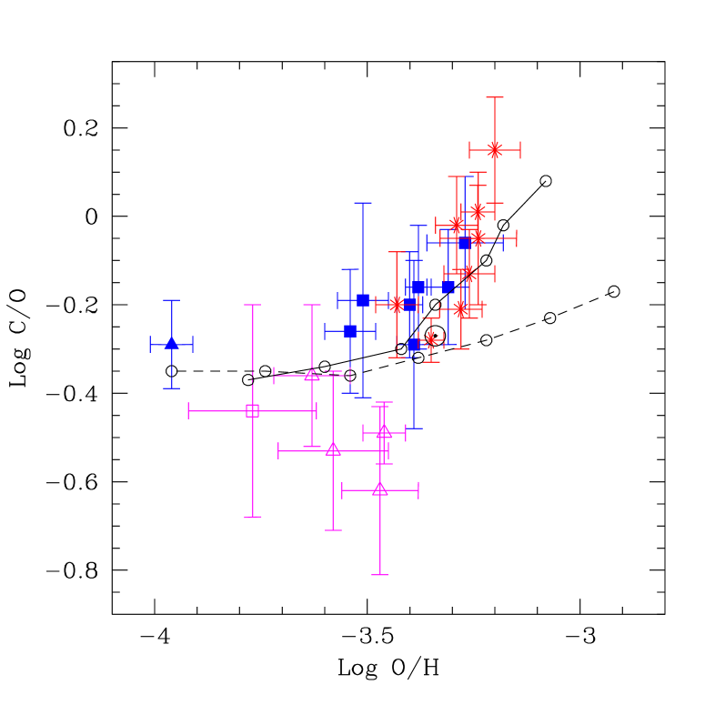
Figure 4: C/O vs. O/H ratios of Galactic and extragalactic H II regions (EHRs) determined from recombination lines. Filled (blue) symbols represent the data analysed in this paper; the filled squares correspond to abundance ratios of EHRs in spiral galaxies and the filled triangle to NGC 2363, an EHR in a dwarf galaxy. The empty (magenta) square corresponds to NGC 5471, an EHR at the outskirts of M 101 (data from Esteban et al., 2002). Empty (magenta) triangles correspond to data for EHRs in dwarf galaxies taken from the literature: 30 Dor (Peimbert, 2003), region V of NGC 6822 (Peimbert et al., 2005), and regions A and C of NGC 5253 (López-Sánchez et al., 2007). The (red) asterisks correspond to data for Galactic H II regions (García-Rojas, 2006; García-Rojas & Esteban, 2007). The solar symbol (large circle) represents the abundances of the Sun (Grevesse et al., 2007). The lines show the predictions of chemical evolution models by Carigi et al. (2005) and Carigi & Peimbert (2008) for the present-day Galactic disk at different Galactocentric distances for high-wind yields and M_up = 80 M_⊙ (solid line) and for low-wind yields and M_up = 80 M_⊙ (dashed line). In both lines, the small open circles represent the predictions of the models at different Galactocentric distances, from right to left: 4, 6, 8, 10, 12, 14, and 16 kpc.

6 Conclusions

Echelle spectrophotometry from 3550 to 7440 Å has been obtained with the HIRES spectrograph at the Keck I telescope for 13 extragalactic H II regions (EHRs). One additional object was observed with the WHT telescope at lower spectral resolution. The EHRs observed include objects in the spiral galaxies M 31, M 33, M 83, M 101, NGC 2403, and NGC 4395 as well as in irregular and blue compact dwarf galaxies: NGC 1741, NGC 2366, and NGC 4861.

The spectra are very deep and a number of lines between 38 and 135 have been measured in each EHR. We detected C II lines in 10 of the objects and O II lines in 8 of them. This allows us to derive the C⁺⁺ and O⁺⁺ abundances from recombination lines, which are independent of possible variations of the spatial distribution of the electron temperature in the nebulae.

We have obtained a large number of different $T_{\rm e}$ determinations, in particular those associated with low ionization potential ions: [N II], [O II], and [S II]. We have obtained a rather tight empirical linear relation between $T_{\rm e}$([N II]) and $T_{\rm e}$([O III]), which is almost identical to the relationship found by Garnett (1992) from photoionization models. The use of this relation is of interest for abundance determinations of H II regions where $T_{\rm e}$([O III]) can not be determined. A linear relationship is also found between $T_{\rm e}$([O II]) and $T_{\rm e}$([O III]) and between $T_{\rm e}$([S II]) and $T_{\rm e}$([O III]), but with a larger scatter in this last case.

The O⁺⁺ abundance determined from O II recombination lines is always larger than that determined from collisionally excited lines of [O III] in all the objects where both quantities have been calculated. The mean difference between both abundances –the so-called abundance discrepancy factor (ADF)– is 0.26 $\pm$ 0.09 dex –about a factor of 2, which is also similar to the typical values of this parameter in Galactic H II regions and EHRs from the literature. This result indicates that whatever mechanism is producing the abundance discrepancy in H II regions, it seems independent of the properties of the H II regions and of the parent galaxy.

We have determined the O/H, C/H, and C/O radial gradients in the spiral galaxies: M 33, M 101, and NGC 2403. We find that the C/H gradients are always steeper than those of O/H, producing negative slopes of the C/O gradient. The behavior of these gradients is similar to that of the Milky Way determined by Esteban et al. (2005), and can be reproduced when carbon yields that increase with metallicity owing to stellar winds in massive stars are considered (Carigi et al., 2005; Carigi & Peimbert, 2008). The relation between C/O and O/H in extragalactic and Galactic H II regions shows a rather clear trend, where the C/O ratio shows a strong increase for O abundances between 8.5 and 8.8, indicating that the low- and intermediate-mass stars should be important contributors to the C enrichment at higher metallicities.

We are grateful to the referee of this paper for his/her useful comments. This work has been funded by the Spanish Ministerio de Ciencia y Tecnolog a (MCyT) under project AYA2004-07466, Ministerio de Educación y Ciencia (MEC) under project AYA2007-63030, and the Mexican CONACyT grant 46904. F.B gratefully acknowledges the support from the NSF grant AST-0707911.

References

- Akerman et al. (2004) Akerman, C. J., Carigi, L., Nissen, P. E., Pettini, M., & Asplund, M. 2004, A&A, 414, 931
- Benjamin et al. (2002) Benjamin, R.A., Skillman, E.D. & Smits, D.P. 2002, ApJ, 569, 288
- Bensby & Feltzing (2006) Bensby, T., & Feltzing, S. 2006, MNRAS, 367, 1181
- Bresolin (2006) Bresolin, F. 2006, arXiv:astro-ph/0608410
- Bresolin (2007) Bresolin, F. 2007, ApJ, 656, 186
- Bresolin (2008) Bresolin, F. 2008, IAU Symposium, 250, 273
- Bresolin et al. (2009) Bresolin, F., Gieren, W., Kudritzki, R.-P., Pietrzynski, G., Urbaneja, M., & Carraro, G. 2009, ApJ, submitted
- Bresolin et al. (2005) Bresolin, F., Schaerer, D., González Delgado, R. M., & Stasińska, G. 2005, A&A, 441, 981
- Campbell et al. (1986) Campbell, A., Terlevich, R., & Melnick, J. 1986, MNRAS, 223, 811
- Carigi & Peimbert (2008) Carigi, L., & Peimbert, M. 2008, Revista Mexicana de Astronomia y Astrofisica, 44, 341
- Carigi et al. (2005) Carigi, L., Peimbert, M., Esteban, C., & García-Rojas, J. 2005, ApJ, 623, 213
- Cedrés & Cepa (2002) Cedrés, B., & Cepa, J. 2002, A&A, 391, 809
- Conti & Massey (1981) Conti, P. S., & Massey, P. 1981, ApJ, 249, 471
- Crockett et al. (2006) Crockett, N. R., Garnett, D. R., Massey, P., & Jacoby, G. 2006, ApJ, 637, 741
- Davey et al. (2000) Davey, A. R., Storey, P. J., & Kisielius, R. 2000, A&AS, 142, 85
- de Vaucouleurs et al. (1976) de Vaucouleurs, G., de Vaucouleurs, A., & Corwin, H. G. 1976, University of Texas Monographs in Astronomy, Austin: University of Texas Press, 1976.
- de Vaucouleurs et al. (1991) de Vaucouleurs, G., de Vaucouleurs, A., Corwin, H. G., Jr., Buta, R. J., Paturel, G., & Fouque, P. 1991, Volume 1-3, XII, 2069 pp. 7 figs.. Springer-Verlag Berlin Heidelberg New York, 1991.
- Dinerstein & Shields (1986) Dinerstein, H. L., & Shields, G. A. 1986, ApJ, 311, 45
- Esteban et al. (2005) Esteban, C., García-Rojas, J., Peimbert, M., Peimbert, A., Ruiz, M. T., Rodríguez, M., & Carigi, L. 2005, ApJ, 618, L95
- Esteban et al. (2004) Esteban, C., Peimbert, M., García-Rojas, J., Ruiz, M. T., Peimbert, A., & Rodríguez, M. 2004, MNRAS, 355, 229
- Esteban et al. (1998) Esteban, C., Peimbert, M., Torres-Peimbert, S., & Escalante, V. 1998, MNRAS, 295, 401
- Esteban et al. (2002) Esteban, C., Peimbert, M., Torres-Peimbert, S., & Rodríguez, M. 2002, ApJ, 581, 241
- Fierro et al. (1986) Fierro, J., Torres-Peimbert, S., & Peimbert, M. 1986, PASP, 98, 1032
- Freedman et al. (2001) Freedman, W. L., et al. 2001, ApJ, 553, 47
- Froese Fischer et al. (2008) Froese Fischer, C., Rubin, R. H., & Rodríguez, M. 2008, MNRAS, 391, 1828
- Galarza et al. (1999) Galarza, V. C., Walterbos, R. A. M., & Braun, R. 1999, AJ, 118, 2775
- García-Rojas (2006) García-Rojas, J. 2006, PhD thesis, Universidad de La Laguna
- García-Rojas & Esteban (2007) García-Rojas, J., & Esteban, C. 2007, ApJ, 670, 457
- García-Rojas et al. (2005) García-Rojas, J., Esteban, C., Peimbert, A., Peimbert, M., Rodríguez, M., & Ruiz, M. T. 2005, MNRAS, 362, 301
- García-Rojas et al. (2007) García-Rojas, J., Esteban, C., Peimbert, A., Rodríguez, M., Peimbert, M., & Ruiz, M. T. 2007, Rev. Mexicana Astron. Astrofis., 43, 3
- García-Rojas et al. (2006) García-Rojas, J., Esteban, C., Peimbert, M., Costado, M. T., Rodríguez, M., Peimbert, A., & Ruiz, M. T. 2006, MNRAS, 368, 253
- García-Rojas et al. (2004) García-Rojas, J., Esteban, C., Peimbert, M., Rodríguez, M., Ruiz, M. T., & Peimbert, A. 2004, ApJS, 153, 501
- Garnett (1992) Garnett, D. R. 1992, AJ, 103, 1330
- Garnett et al. (1999) Garnett, D.R., Shields, G.A., Peimbert, M., Torres-Peimbert, S., Skillman, E.D., Dufour, R.J., Terlevich, E. & Terlevich, R.J. 1999, ApJ, 513, 168
- Garnett et al. (1997) Garnett, D. R., Shields, G. A., Skillman, E. D., Sagan, S. P., & Dufour, R. J. 1997, ApJ, 489, 63
- Garnett et al. (1995) Garnett, D. R., Skillman, E. D., Dufour, R. J., Peimbert, M., Torres-Peimbert, S., Terlevich, R., Terlevich, E., & Shields, G. A. 1995, ApJ, 443, 64
- Gil de Paz et al. (2003) Gil de Paz, A., Madore, B. F., & Pevunova, O. 2003, ApJS, 147, 29
- González-Delgado et al. (1994) González-Delgado, R. M., et al. 1994, ApJ, 437, 239
- Grevesse et al. (2007) Grevesse, N., Asplund, M., & Sauval, A. J. 2007, Space Science Reviews, 130, 105
- Hägele et al. (2006) Hägele, G. F., Pérez-Montero, E., Díaz, Á. I., Terlevich, E., & Terlevich, R. 2006, MNRAS, 372, 293
- Hägele et al. (2008) Hägele, G. F., Díaz, Á. I., Terlevich, E., Terlevich, R., Pérez-Montero, E., & Cardaci, M. V. 2008, MNRAS, 383, 209
- Hickson (1982) Hickson, P. 1982, ApJ, 255, 382
- Hirschi et al. (2005) Hirschi, R., Meynet, G., & Maeder, A. 2005, A&A, 433, 1013
- Hodge et al. (1990) Hodge, P. W., Gurwell, M., Goldader, J. D., & Kennicutt, R. C., Jr. 1990, ApJS, 73, 661
- Hummer & Storey (1987) Hummer, D. G., & Storey, P. J. 1987, MNRAS, 224, 801
- Izotov et al. (1994) Izotov, Y.I., Thuan, T.X., & Lipovetski, 1994
- Johansson et al. (2000) Johansson, S., Zethson, T., Hartman, H., Ekberg, J. O., Ishibashi, K., Davidson, K., & Gull, T. 2000, A&A, 361, 977
- Kamphuis (1993) Kamphuis, J. J. 1993, Ph.D. Thesis, Univ. Groningen
- Kennicutt et al. (2003) Kennicutt, R. C., Jr., Bresolin, F., & Garnett, D. R. 2003, ApJ, 591, 801
- Kennicutt & Garnett (1996) Kennicutt, R. C., Jr., & Garnett, D. R. 1996, ApJ, 456, 504
- Kingdon & Ferland (1995) Kingdon, J. & Ferland, G.J. 1995, ApJ, 442, 714
- Kobulnicky & Skillman (1998) Kobulnicky, H. A., & Skillman, E. D. 1998, ApJ, 497, 601
- Liu (2006) Liu, X.-W. 2006, Planetary Nebulae in our Galaxy and Beyond, 234, 219
- Liu et al. (2000) Liu, X.-W., Storey, P. J., Barlow, M. J., Danziger, I. J., Cohen, M., & Bryce, M. 2000, MNRAS, 312, 585
- López-Sánchez et al. (2006) López-Sánchez, Á. R., Esteban, C., & García-Rojas, J. 2006, A&A, 449, 997
- López-Sánchez et al. (2007) López-Sánchez, A. R., Esteban, C., García-Rojas, J., Peimbert, M., & Rodríguez, M. 2007, ApJ, 656, 168
- López-Sánchez et al. (2004) López-Sánchez, Á. R., Esteban, C., & Rodríguez, M. 2004, ApJS, 153, 243
- Maeder (1992) Maeder, A. 1992, A&A, 264, 105
- Magrini et al. (2007) Magrini, L., Vílchez, J. M., Mampaso, A., Corradi, R. L. M., & Leisy, P. 2007, A&A, 470, 865
- Mazzarella & Boroson (1993) Mazzarella, J.M. & Boroson, T.A. 1993, ApJS, 85, 27
- McCall et al. (1985) McCall, M. L., Rybski, P. M., & Shields, G. A. 1985, ApJS, 57, 1
- Mesa-Delgado et al. (2009) Mesa-Delgado, A., Esteban, C., García-Rojas, J., Luridiana, V., Bautista, M., Rodríguez, M., López-Marín, L., & Peimbert, M. 2009, MNRAS, in press
- Meynet & Maeder (2002) Meynet, G., & Maeder, A. 2002, A&A, 390, 561
- Meynet & Maeder (2005) Meynet, G., & Maeder, A. 2005, A&A, 429, 581
- Peimbert (2003) Peimbert, A. 2003, ApJ, 584, 735
- Peimbert et al. (2002) Peimbert, A., Peimbert, M. & Luridiana, V. 2002, ApJ, 565, 688
- Peimbert et al. (2005) Peimbert, A., Peimbert, M., & Ruiz, M. T. 2005, ApJ, 634, 1056
- Peimbert & Costero (1969) Peimbert M. & Costero, R. 1969, Bol. Obs. Tonantzintla y Tacubaya, 5, 3
- Peimbert et al. (1992) Peimbert, M., Torres-Peimbert, S., & Ruiz, M.T. 1992, Rev. Mex. Astron. Astrofís., 24, 155
- Peimbert et al. (2000) Peimbert, M., Peimbert, A., & Ruiz, M.T. 2000, ApJ, 541, 688
- Peimbert et al. (2007) Peimbert, M., Peimbert, A., Esteban, C., García-Rojas, J., Bresolin, F., Carigi, L., Ruiz, M. T., & López-Sánchez, A. R. 2007, Revista Mexicana de Astronomia y Astrofisica Conference Series, 29, 72
- Pérez-Montero & Díaz (2003) Pérez-Montero, E., & Díaz, A. I. 2003, MNRAS, 346, 105
- Pilyugin et al. (2006) Pilyugin, L. S., Vílchez, J. M., & Thuan, T. X. 2006, MNRAS, 370, 1928
- Porter et al. (2005) Porter, R. L., Bauman, R. P., Ferland, G. J., & MacAdam, K. B. 2005, ApJ, 622, L73
- Porter et al. (2007) Porter, R. L., Ferland, G. J., & MacAdam, K. B. 2007, ApJ, 657, 327
- Rayo et al. (1982) Rayo, J. F., Peimbert, M., & Torres-Peimbert, S. 1982, ApJ, 255, 1
- Quinet (1996) Quinet, P. 1996, A&AS, 116, 573
- Rodríguez (1999) Rodríguez, M. 1999, A&A, 348, 222
- Rodríguez & Rubin (2005) Rodríguez, M. & Rubin, R.H. 2005, ApJ, 626, 900
- Rosolowsky & Simon (2008) Rosolowsky, E., & Simon, J. D. 2008, ApJ, 675, 1213
- Ruiz et al. (2003) Ruiz, M. T., Peimbert, A., Peimbert, M., & Esteban, C. 2003, ApJ, 595, 247
- Sakai et al. (2004) Sakai, S., Ferrarese, L., Kennicutt, R. C., Jr., & Saha, A. 2004, ApJ, 608, 42
- Salzer et al. (2005) Salzer, J. J., Lee, J. C., Melbourne, J., Hinz, J. L., Alonso-Herrero, A., & Jangren, A. 2005, ApJ, 624, 661
- Sawey & Berrington (1993) Sawey, P. M. J., & Berrington, K. A. 1993, Atomic Data and Nuclear Data Tables, 55, 81
- Seaton (1979) Seaton, M. J., 1979, MNRAS, 187, 73
- Shaw & Dufour (1995) Shaw, R. A., & Dufour, R. J. 1995, PASP, 107, 896
- Smith et al. (1996) Smith, L.F., Shara, M.M. & Moffat, A.F.J. 1996, MNRAS, 281, 163
- Stasińska (1978) Stasińska, G. 1978, A&A, 66, 257
- Stasińska (1990) Stasińska, G. 1990, A&AS, 83, 501
- Stasińska (2005) Stasińska, G. 2005, A&A, 434, 507
- Stasińska et al. (2007) Stasińska, G., Tenorio-Tagle, G., Rodríguez, M., & Henney, W. J. 2007, A&A, 471, 193
- Storey (1994) Storey, P. J. 1994, A&A, 282, 999
- Storey & Hummer (1995) Storey, P. J., & Hummer, D. G. 1995, MNRAS, 272, 41
- Torres-Peimbert et al. (1989) Torres-Peimbert, S., Peimbert, M., & Fierro, J. 1989, ApJ, 345, 186
- Tsamis et al. (2003) Tsamis, Y. G., Barlow, M. J., Liu, X.-W., Danziger, I. J., & Storey, P. J. 2003, MNRAS, 338, 687
- Tsamis & Péquignot (2005) Tsamis, Y. G., & Péquignot, D. 2005, MNRAS, 364, 687
- Urbaneja et al. (2005) Urbaneja, M. A., Herrero, A., Kudritzki, R.-P., Najarro, F., Smartt, S. J., Puls, J., Lennon, D. J., & Corral, L. J. 2005, ApJ, 635, 311
- van Zee et al. (1998) van Zee, L., Salzer, J. J., Haynes, M. P., O’Donoghue, A. A., & Balonek, T. J. 1998, AJ, 116, 2805
- Verner et al. (2000) Verner, E.M., Verner, D.A., Baldwin, J.A., Ferland, G.J. & Martin, P.G. 2000, ApJ, 543, 831
- Véron & Sauvayre (1965) Véron, P., & Sauvayre, A. 1965, Annales d’Astrophysique, 28, 698
- Vílchez et al. (1988) Vílchez, J. M., Pagel, B. E. J., Diaz, A. I., Terlevich, E., & Edmunds, M. G. 1988, MNRAS, 235, 633
- Vogt et al. (1994) Vogt, S. S., et al. 1994, Proc. SPIE, 2198, 362
- Walterbos & Braun (1992) Walterbos, R. A. M., & Braun, R. 1992, A&AS, 92, 625
- Zaritsky et al. (1989) Zaritsky, D., Elston, R., & Hill, J. M. 1989, AJ, 97, 97
- Zaritsky et al. (1994) Zaritsky, D., Kennicutt, R. C., Jr., & Huchra, J. P. 1994, ApJ, 420, 87
- Zhang (1996) Zhang, H. L. 1996, A&AS, 119, 523
- Zhang & Pradhan (1997) Zhang, H. L., & Pradhan, A. K. 1997, A&AS, 126, 373