The state of a non-relativistic gravitational dynamical system is known at any time $t$ if the dynamical rule, i.e. Newton’s equations of motion, can be solved; this requires specification of the gravitational potential. The evolution of a bunch of phase space coordinates ${\bf w}$ is deterministic, though generally non-linear. We discuss the novel Bayesian non-parametric algorithm CHASSIS that gives phase space $pdf$ $f({\bf w})$ and potential $\Phi({\bf x})$ of a relaxed gravitational system. CHASSIS is undemanding in terms of input requirements in that it is viable given incomplete, single-component velocity information of system members. Here ${\bf x}$ is the 3-D spatial coordinate and ${\bf w}={\bf x+v}$ where ${\bf v}$ is the 3-D velocity vector. CHASSIS works with a 2-integral $f=f(E,L)$ where energy $E=\Phi+v^{2}/2,\>v^{2}=\sum_{i=1}^{3}{v_{i}^{2}}$ and the angular momentum is $L=|{\bf r}\times{\bf v}|$, where ${\bf r}$ is the spherical spatial vector. Also, we assume spherical symmetry. CHASSIS obtains the $f(\cdot)$ from which the kinematic data is most likely to have been drawn, in the best choice for $\Phi(\cdot)$, using an MCMC optimiser (Metropolis-Hastings). The likelihood function ${\cal{L}}$ is defined in terms of the projections of $f(\cdot)$ into the space of observables and the maximum in ${\cal{L}}$ is sought by the optimiser. The recovered solutions can be susceptible to large uncertainties given the dimensionality of the domain of the unconstrained $f(\cdot)$ and the typically small, observed velocity samples in distant astrophysical systems. This scenario is tackled by assuming $f=f(E)$, i.e. we assume the phase space to be isotropic. However, this simplifying assumption of isotropy is addressed by undertaking a Bayesian test of significance that is developed to be used in the non-parametric context.

A test based on the $p$-value estimates of the goodness of isotropy in the data was previously undertaken (Chakrabarty $\&$ Saha 2001). However, $p$-values are sensitive to sample sizes and obfuscate interpretation of analyses of differently sized kinematic samples. Thus, a Bayesian formalism is a better alternative, eg. Fully Bayesian Significance Test or FBST (Pereira $\&$ Stern 1999, Pereira, Stern $\&$ Wechsler 2008). The null hypothesis that we aim to test, is that the data are drawn from an isotropic $f(\cdot)$, i.e. $H_{0}:{\hat{f}}=\Psi[E(v^{2}/2+\Phi(r))]$ where the data are drawn from $\hat{f}$ and $\Psi$ is some function: $\Psi>0$ for $E<0$ and $\Psi=0$ otherwise. Within FBST, the evidence value ($ev$) in favour of $H_{0}$ is obtained by first numerically spotting the most likely configuration ($\theta^{*}$) that is compatible with $H_{0}$ and then finding the volume of the tangential set $T$ by numerical integration. Here $T$ is the set of all configurations with posterior probability in excess of that of $\theta^{*}$. We have developed the implementation of this scheme in the non-parametric context; in CHASSIS, the configurations are $f(E)$ and $\Phi(r)$. To have configurations obeying $H_{0}$, we perform sampling from the $f(E)-\Phi(r)$ pair identified upon convergence of a run of CHASSIS. From this sampling, the resulting $f(E)-\Phi(r)$ configuration corresponding to the highest ${\cal{L}}$ is compared to all the other $f(E)-\Phi(r)$ pairs, in order to obtain a measure of the volume of $T$.

We discuss two distinct applications of the isotropic version of CHASSIS. In one, 2 distinct kinematic data sets of 2 distinct types of members of an example galaxy are analysed by CHASSIS under the assumption of isotropy. The $f(\cdot)$ and $\Phi(\cdot)$ recovered from runs done with the two data sets are identified as distinct. Given that the same galaxy cannot be described by two different gravitational potentials, the risk involved in the very method of extracting the galactic potential from kinematic data of individual galactic members is demonstrated here for the first time. The goodness of the assumption of isotropy, given the 2 data sets, is quantified by our Bayesian test of hypothesis.

In the second application, it is shown that once the amount of gravitational matter inside a fiduciary radius is pinned down from independent measurements, the recovered $\Phi(\cdot)$ is unique, irrespective of the toy $f(\cdot)$, from which kinematic data samples are drawn as input for CHASSIS, as long as velocity dispersion values are measured at 1 or more different locations in the system. This consistent nature of $\Phi(\cdot)$ is arrived at, notwithstanding varied forms for the assumed toy $f(\cdot)$, including isotropic as well as $E\>\&\>L$ dependent forms.

Keywords: Bayes theorem, Bayesian significance test, Astrophysical applications.

1 Introduction

The complete characterisation of a gravitationally bound, non-relativistic dynamical system can be undertaken with the help of $f({\bf{w}},t)$ - the $pdf$ of phase space $W$ - and the gravitational potential $\Phi(\bf{x})$; here $t$ is time and ${\bf{w=x+v}}$, where ${\bf{x}}$ represents the spatial coordinates and the velocity vector is ${\bf{v}}={\bf{\dot{x}}}$. A sample of phase space coordinates can be drawn from $f(\cdot)$ and allowed to evolve in $\Phi(\cdot)$, in accordance to Newton’s laws. In this way, the evolution of the system is deterministic at any time $t$, though non-linear in general. Hence, we aim to estimate $f(\cdot)$ and $\Phi(\cdot)$; we focus on the characterisation of astrophysical systems in this paper. A related aim is to derive the distribution of the total gravitating matter from the estimated $\Phi(\cdot)$, while keeping in mind that such $total$ mass is accounted for only partly by luminous matter while the greater fraction is dark matter in these systems.

Conventionally,

• $f(\cdot)$ and $\Phi(\cdot)$ are almost always parametrically described. However, given that astrophysical systems such as galaxies are more likely to manifest complexity in their dynamics than otherwise, any smooth parametric description of such systems is erroneous.

• mass determination is typically pursued via observed photometric or luminous information though no functional dependence of the total (luminous+dark) matter content on such measurements exist.

• inhomogeneities in the measurement errors notwithstanding, goodness-of-fit parameters are often invoked to seek the solution. For galaxies, measurements are typically noisy and such goodness-of-fit parameters can be artificially inflated (Bissantz $\&$ Munk, 2001).

All these issues suggest a better - preferably, a nonparametric - route to $f(\cdot)$ and $\Phi(\cdot)$ determination. It is such a novel, data driven characterisation of real (as distinguished from simulated) astrophysical systems that CHASSIS offers, using the few kinematic measurements that are typically available. Importantly, we test the chief assumption of our algorithm using a test of significance that is developed in this regard.

As motivated above, we discard all photometric information that may be available for a system at hand and use the kinematic information that is sometimes available, namely velocities along the line-of-sight (LOS) of individual system members, (such as stars). We define the galaxy such that the $x_{1}-x_{2}$ coordinate system spans the plane-of-the-sky (POS) and the LOS is along the z-axis. Thus, our data comprise 1-component $v_{3}$ values of individual galactic members and their POS coordinates. We also account for the errors in $v_{3}$ measurement. The observed data samples often bear $\lesssim$ 100 data points. These data are input into the Bayesian algorithm CHASSIS (Chakrabarty $\&$ Saha 2001, Chakrabarty $\&$ Portegies Zwart 2005).

2 CHASSIS

CHASSIS helps constrain $\Phi(\cdot)$ and $f(\cdot)$ of galaxies, given the data $u$ (say). Actually, within CHASSIS, we constrain the gravitational matter density $\rho({\cdot})$ rather than $\Phi(\cdot)$, where Poisson equation connects $\rho(\cdot)$ and $\Phi(\cdot)$ as in:

$$\Phi(\bf{x})=-4\pi G\nabla^{2}\rho(\bf{x})$$ (1)

This helps to avoid problems about negative $\rho(\cdot)$. The calculation of $\Phi(\cdot)$ from $\rho(\cdot)$ is undertaken at every step.

Dynamical theory tells us (Dubrovin, Fomenko $\&$ Petrovich, 1990):

$$f=f[{K_{i}({\bf{w}})}],\quad{\textrm{where}}\quad\dot{{K_{i}}}=0\quad\forall i=1,2,3\ldots.$$ (2)

i.e. ${K_{i}}$ is an integral of motion. Now, we realise that the size of the data $u$ is small to moderate and typically bears no more information other than a single component of velocity. In such a case, we feel that the data are not sufficient to constrain the extended forms of $f(\cdot)$ and $\Phi(\cdot)$. In other words, we resort to making assumptions about $f(\cdot)$ and $\Phi(\cdot)$.

In fact, we assume $K_{i}\neq$constant, only for $i=1,2$. Thus, $f=f[K_{1}({\bf w}),K_{2}({\bf w})]$ where $K_{1}\equiv$energy $E$ of the galactic particle and $K_{2}\equiv$ the angular momentum or $L$. Here $E=\sum_{j}v_{j}^{2}/2+\Phi({\bf x})$ and $L=|{\bf r}\times{\bf v}|$ where ${\bf r}$ is the spherical radius and ${\bf v}$ is the 3-D velocity vector: $\sum_{j}x_{j}^{2}=r^{2}$, $v^{2}=\sum_{j}v_{j}^{2}$. We also assume radial symmetry in the potential, i.e. $\Phi({\bf x})=\Phi(r)$. Thus, the particle energy is $E=v^{2}/2+\Phi(r)$. In this geometry, the Poisson equation (Equation 1) is solved numerically by assuming the mass to be stratified on spherical shells. In other words, the relevant radial range is discretised and over each radial bin, $\rho(r)$ is held a constant.

In this background, we seek

$$\Pr(f,\rho|u)\propto\Pr(u|f,\rho)\Pr(f,\rho)$$ (3)

where the only constraints posed by the priors are physically realistic requirements of positivity and monotonicity. This owes to the fact that in general, we do not possess any other prior information that could help constrain the forms of the sought functions. Thus,

$$\Pr(f,\rho) = \Pr(f)\Pr(\rho),\quad{\textrm{where}}$$

$$\Pr(f) = 1\quad{\textrm{if}}\quad f\geq 0\>\vee{\displaystyle{\frac{\partial f}{\partial E}{\bigg{|}}_{L}\leq 0}}$$

$$= 0\quad{\textrm{otherwise}}$$

$$\Pr(\rho) = 1\quad{\textrm{if}}\quad\rho\geq 0\>\vee{\displaystyle{\frac{d\rho}{dr}\leq 0}}$$ (4)

$$= 0\quad{\textrm{otherwise}}$$

We adopt the above priors and estimate the $f(\cdot)$ from which the data $u$ is most likely to have been drawn, in the estimated $\Phi(\cdot)$. This is done by iterating towards the most likely set of $\{f(\cdot),\rho(\cdot)\}$ starting with an arbitrarily chosen seed. At every step, the current choice of $f(\cdot)$ is projected into the space of observables (spanned by $x_{1},x_{2},v_{3}$); a ready definition for the likelihood function ${\cal{L}}$ is in terms of the projection $\eta(\cdot)$ of $f(E,L)$.

$$\eta_{i}(x_{1}^{i},x_{2}^{i},v_{3}^{i}) = \displaystyle\int{f[E(v,\Phi(r)),\>L]\>dx_{3}dv_{1}dv_{2}}\quad{\textrm{and}}$$

$${\cal{L}} = \displaystyle{\sum_{i=1}^{N_{data}}\log\eta_{i}}$$ (5)

where $x_{1}^{i},x_{2}^{i},v_{3}^{i}$ is the $i^{th}$ data point in the $N_{data}$ sized data sample.

The numerical implementation of a trial $f(\cdot)$ function, at a trial ($\rho(\cdot)$ or) $\Phi(\cdot)$ is the crucially important question from the point of view of algorithm design. We do this by discretising the $E-L$ space and holding $f(\cdot)$ a constant (=$f_{cell}$) over a given $E-L$ cell. The contribution to $\eta(\cdot)$, from this $E-L$ cell - defined by say, $E\in[E_{1},E_{2}],\>L\in[L_{1},L_{2}]$ - is given as:

$$\eta_{i}^{cell} = \displaystyle{f_{cell}\int{dx_{3}dv_{1}dv_{2}}}\quad{\textrm{and}}$$

$$\eta_{i} = \displaystyle{\sum_{cell}\eta_{i}^{cell}}$$ (6)

Let the integral on the right hand side of the former of these two equations be $A$. Then, we seek the mapping $A:\longrightarrow E-L$space.

In order to establish this, first we determine the 2-D area of intersection between the locii of $E=E_{1}$, $E=E_{2}$, $L=L_{1}$, $L=L_{2}$, in the $v_{1}-v_{2}$ space. This gives the connection between the $E-L$ cell at hand and $v_{1},v_{2}$. Mapping $x_{3}$ to this cell requires knowledge of the minimum and maximum values of $x_{3}$ that are allowed in the cell, given the data point $x_{1}^{i},x_{2}^{i},v_{3}^{i}$. This maximum value is $\sqrt{r_{0}^{2}-(x_{1}^{i})^{2}-(x_{2}^{i})^{2}}$ where $r_{0}$ is the solution to: $E_{2}=v_{3}^{2}/2+L^{2}/2r_{0}^{2}+\Phi(r_{0})$. The minimum $x_{3}$ is 0.

This explains the background to the structures of $\rho(\cdot)$ and $f(\cdot)$.

2.1 $\rho$-histogram and $f$-histogram

The representation of $f(E,L)$ over the discretised $E-L$ space, is akin to a 2-D histogram. Similarly, the $\rho(r)$ structure is represented as a 1-D histogram. These histograms are updated at the beginning of every step, while maintaining positivity and monotonicity.

The jump distribution we use is discussed below. If in step $k$, for $r\in[r_{q-1},r_{q}]$ ($\forall q=1,\ldots,N_{r}$, $r_{0}$=0), $\rho(r_{q})=\alpha_{q}^{k}$, then in the $k+1^{th}$ step:

$$\alpha_{q}^{k+1}=\alpha_{q+1}^{k}+\displaystyle{(\alpha_{q}^{k}-\alpha_{q+1}^{k})\exp\left(\frac{{\cal R}}{s_{1}}\right)}$$ (7)

where ${\cal R}$ is a random number with ${\cal R}\in[-0.5,0.5]$ and $s_{1}$ is an experimentally optimised scale that determines the scale over which the shape of the $\rho$-histogram is changed. This updating is done $\forall q$. Once the shape of the $\rho$-histogram is updated in this way, the whole structure is scaled by the factor $\exp({\cal R}/s_{2})$ where $s_{2}$ is another scale. The $f$-histogram is similarly updated in shape and subsequently normalised.

2.2 Optimisation

Once the histograms are updated, we project the current $f(\cdot)$ over an $E-L$ cell, into the space of observables, for the $i^{th}$ data point and then sum over all such cells to get $\eta_{i}$ (Equation 7). This is done $\forall\>i$, to obtain ${\cal L}$ (Equation 6). The global maxima in ${\cal L}$ is sought by the Metropolis-Hastings algorithm (Metropolis et. al 1953, Hastings 1970, Chib $\&$ Greenberg 1995). Anticipating the likelihood distribution to be multimodal, we work with highly dispersed seeds to initiate several chains (Gelman $\&$ Rubin 1992) as well as employ simulated annealing on a single chain. The latter approach, though perhaps less obvious, is one that we find very effective in test runs.

While the optimisation routine is hard-wired within CHASSIS, the user is allowed the flexibility to adjust details of the used cooling schedule and other optimisation parameters such as the scales relevant to the jump distribution ($s_{1}$, $s_{2}$). In this note, it is worth mentioning that the current implementation of optimisation is modular, and it is simple to replace it by a more effcient routine.

2.3 Required User Input

The methodology discussed above is incorporated into CHASSIS and all that user is required to input is the velocity data, the source of which is independent of CHASSIS. Thus, measured kinematic data, irrespective of its source, is acceptable, as long as the columns pertain to the observables $r_{p}$, $v_{3}$ and the measured errors in $v_{3}$. Here $r_{p}=\sqrt{x_{1}^{2}+x_{2}^{2}}$. Besides, the user is allowed to input details such as the number of bins, bin widths, fraction of data she wants to perform the run with, the seeds for the sought solutions and the optimisation related details (see Section 2.2). The user inputs are advanced via an input file that CHASSIS calls at the beginning of a run.

2.4 Assumption of Isotropy

Given the limited data sample, we find that limiting the domain of $f$ to 2-D is not constraining enough in reducing the magnitude of uncertainties in the estimated solutions to useful levels. Thus, we resort to imposing the further constraint that $f=f(E)$, i.e. we assume isotropy to exist in phase space (since $E$ is symmetrical in $v_{j}$ and $x_{j}$, where $j$=1,2,3). Then we resort to (1) justifying or rejecting our assumption in the data by performing a test of hypothesis exercise (2)exploring independent measurements that may be available in the literature to obtain a $\rho$ that is unaffected by the amount of anisotropy in the data.

3 Testing for Isotropy - Nonparametric FBST

We test for isotropy in the data, i.e. the null hypothesis $H_{0}:{\hat{f}}=\Psi[E(v,r)]$, where ${\hat{f}}$ is the phase space $pdf$ from which the observed data are drawn and $\Psi$ is some function that manifests phase space isotropy: $\Psi(E)=0\forall E>0$ and $\Psi(E)>0$ otherwise.

This $H_{0}$ is tested in the data $u$ along the lines of the Fully Bayesian Significance Test or FBST (Pereira $\&$ Stern 1999; Pereira, Stern $\&$ Wechsler 2008), except that here, we advance a nonparametric implementation of the same. Our null is sharp, as is the requirement for FBST (Madurga, Esteves $\&$ Wechsler 2001). We refer to our object functions $\{\rho(\cdot),f(\cdot)\}\equiv\theta$ (say); let $\theta\in\Theta$-space. We assume that $\theta$ is continuous in the $\Theta$-space. According to FBST, the evidence in favour of $H_{0}$ is $1-ev$, where:

$$ev = 1-\Pr(\theta\in T|u),\quad{\textrm{where}}\quad$$

$$T = \{\theta:\Pr(\theta|u)>\Pr(\theta^{*}|H_{0})\}.$$ (8)

Here $\theta^{*}$ is the value of $\theta$ which, under the null, maximises the posterior $\Pr(\theta|u)$.

At the end of every iterative step during a run of CHASSIS, a $\theta$ configuration is identified. The $f(\cdot)$ recovered upon convergence of the run is indeed a function of $E$ and $E$ only but the true ${\hat{f}}$ is not necessarily so.

Upon convergence of a run of CHASSIS performed with data $u$, we sample the recovered $\theta$, $N$ times, such that the $i^{th}$ sampling of $\theta$ gives the $i^{th}$ set of observables or $u_{i}$; $i=1,2,\ldots,N$. These $N$ data samples are then input into $N$ different new runs of the algorithm. During the run performed with the data $u_{i}$, the $j^{th}$ iterative step yields the configuration $\theta_{i}^{j}$ (say), where $\theta_{i}^{j}\equiv\{f(\cdot)_{i}^{j},\rho(\cdot)_{i}^{j}\}$. Then $f(\cdot)_{i}^{j}$ is isotropic $\forall i,j$, since the phase space $pdf$ from which $u_{i}$ is drawn is the recovered $f(E)$, which by construction, is indeed isotropic.

We scan over all $i,j$ to identify $i^{*},j^{*}$ for which the posterior is maximised. Thus, $\theta_{i^{*}}^{j^{*}}=\theta^{*}$ is identified. Here $\theta^{*}\equiv\{f^{*}(E),\>\rho^{*}(r)\}$, i.e. functions recovered at the end of the $j^{*}$-th step, in a run performed with the data $u_{i^{*}}$.

In this nonparametric implementation, $\Pr(\theta\in T|u)=X/Y$, where $X$ is the number of times that a step yields a likelihood in excess of $\Pr(\theta^{*}|H_{0})$ in all the undertaken runs. $Y$ is the total number of iterative steps in all the runs undertaken.

4 Application 1 - multistability in galaxies

It is a common practise in astrophysics to employ the measured 1-D velocity data of suitable galactic members, with the aim of recovering the total gravitational mass distributions. To examine the viability of such a practise, we employ the available measured kinematic data of two distinct classes of galactic members in an example galaxy - as an aside, these are planetary nebulae (PNe) and globular clusters (GCs). The data of 164 PNe ($u_{P}$) are due to Douglas et al (2007) and that of 30 GCs ($u_{G}$) are due to Bergond et. al (2006). These sample sizes are too discrepant to allow for easy interpretation of any $p$-value based testing of $H_{0}$ defined in Section 3. Instead, we resort to the non-parametric FBST discussed above.

$\begin{array}[]{c c}\includegraphics[height=130.82742pt]{compare_2.ps}&\includegraphics[height=130.82742pt]{fbst_2.ps}\end{array}$

Figure 1: Left: The (normalised) phase space distribution functions recovered from two runs of CHASSIS, performed with the GC data $u_{G}$ (in black) and PNe data $u_{P}$ (in red). The normalisation is performed to ensure that $f(E)$=1 for $E$=-1. These $pdf$s are recovered under the assumption of isotropy and our implementation of nonparametric FBST shows that the profile in black is expected to be closer to the true phase space $pdf$ than is the profile in red. The errors are $\pm$1-$\sigma$ uncertainties identified on the solution by the optimiser. Middle: Gravitational matter density distributions from three runs with $u_{G}$ performed with three different seeds (in magenta, cyan and black) and from 3 runs with $u_{P}$ (in yellow, red and blue). The units of density and radius are astrophysical. Right: $\rho(r)$ from one of the runs done with $u_{G}$ is shown in black while that with $u_{P}$ is in red. The $\rho^{*}(r)$ corresponding to the implementation of data $u_{G}$ is shown in green while that corresponding to $u_{P}$ is in blue. We notice that $\rho_{G}(r)$ is consistent with $\rho^{*}(r)$ obtained from $u_{G}$ while $\rho^{*}(r)$ obtained from $u_{P}$ is significantly lower than $\rho_{P}(r)$.

The two data sets are input into the isotropy-assuming and sphericity-assuming CHASSIS. The $f(E)$ and $\rho(r)$ recovered from the two distinct data are found to be inconsistent with each other, within error bars (Figure 1). The difference in the recovered $f(\cdot)$ could arise from different divergences between an isotropic phase space $pdf$ and the ${\hat{f}}$ from which $u_{P}$ are drawn, as compared to that from which $u_{G}$ are drawn. However, the distribution of gravitational matter in the galaxy should be uniquely determined. That such is not our conclusion, prompts us to examine if the inherent assumption of isotropy is to be blamed. Thus, we test for our null $H_{0}$ (defined above in Section 3) in the data $u_{P}$ and $u_{G}$ separately.

The results of our implementation of FBST are shown in Figure 1. We find that for three different runs done with distinct seeds, given $u_{P}$, the average evidence in favour of the null is about 0.60 For three runs done with different seeds, given $u_{G}$, the average $1-ev$ is 0.95. Thus we conclude that the degree of isotropy of the $pdf$ that $u_{G}$ is drawn from is higher than that of the $pdf$ that $u_{P}$ is drawn from.

We wonder if the difference in the recovered mass distributions be due to the concluded difference in isotropy in the two data sets? To understand this, we invoke the peculiarity of CHASSIS that the algorithm overestimates mass density at all $r$ where phase space anisotropy prevails (discussed in Section 5). Thus, we expect that $\rho(r)$ recovered using $u_{P}$ ($\rho_{P}(r)$) is more of an over-estimate compared to the galactic mass density than is the $\rho(r)$ recovered using $u_{G}$ ($\rho_{G}(r)$).

However, as shown in Figure 1, at all $r\gtrsim$ 6 kpc, $\rho_{G}(r)>\rho_{P}(r)$. Therefore, to reconcile the difference between $\rho_{P}(r)$ and $\rho_{G}(r)$, the isotropy issue cannot help unless we propose that $u_{G}$ is drawn from a more anisotropic $pdf$ than $u_{P}$. This is of course not true but its inverse is. Hence we conclude that differences in $\rho_{G}(r)$ and $\rho_{P}(r)$ are intrinsic to the system and not due to our assumption of isotropy.

Thus we have demonstrated the potential risk in employing kinematic data of individual galactic members of a particular population type, to compute the gravitational mass distribution of galaxies. We have also shown that the galactic phase space is described by at least two distinct basins of attractions, i.e. the galaxy is multistable, as we would expect complex systems like galaxies to be.

5 Application 2 - using the total mass constraint

Motivated by the need to simplify our analysis by reducing the number of degrees of freedom to the bare minimum, we persist with the assumption of $f=f(E)$, i.e. phase space is isotropic. We envisage that when the data have been drawn from an anisotropic $pdf$, the algorithm will imply erroneous answers. Using physical arguments we can predict the nature of this error - CHASSIS overestimates $\rho(r)$ at $r$ where phase space anisotropy prevails.

We implement an independent measure of the total gravitational matter ($M_{0}$) inside a given radius ($R_{E}$) in an example galaxy with the aim of recovering the correct solution for $\rho(r)$ under our assumption of isotropy, irrespective of the degree of anisotropy of the $pdf$ from which the input data is drawn. If the system is at a large distance from us, we cannot get velocity data of individual galactic members. Then, we can only get projected velocity dispersion values ($\sigma_{p}$) at 1 or a few radial locations in the galaxy. In this background of sparse and incomplete velocity data, we prepare velocity data samples for inputting to CHASSIS, in the following way.

We select observables ($x_{1},x_{2},v_{3}$) from 3 different toy $f(\cdot)$, two of which are selected to depend on $E$ and $L$ while the third is isotropic. For the example galaxy, $\sigma_{p}$ is known at $r_{1}$, $r_{2}$ and $r_{3}$ say. Then we consider the system to be divided into 3 anulii with $r\in[0,r_{1}],(r_{1},r_{2}],(r_{2},r_{3}]$. The error $\delta$ in the $\sigma_{p}$ measured at $r_{i}$ ($i=1,2,3$) can be related to the size of the data sample $N_{i}$ we intend to draw from the given annulus, assuming normal error distribution. The phase space $pdf$ that we choose our samples from are $f_{Gauss},\>f_{WD}\>f_{Michie}$:

$$f_{Gauss}(E) = \displaystyle{\frac{1}{\sqrt{2\pi\sigma^{2}}}}\displaystyle{exp\left(\frac{-E}{\sigma^{2}}\right)}\quad E<0,$$

$$= 0\quad E>0,$$

$$f_{WD}(E,L) = \displaystyle{\frac{1}{\sqrt{2\pi\sigma^{2}}}}\displaystyle{\exp\left(-\frac{L^{2}}{r_{a}\sigma^{2}}\right)\exp\left(\frac{-E}{\sigma^{2}}\right)}\quad E<0,$$

$$= 0\quad E>0.$$

$$f_{Michie}(E,L) = \displaystyle{\frac{1}{\sqrt{2\pi\sigma^{2}}}}\displaystyle{\exp\left(-\frac{L^{2}}{r_{a}\sigma^{2}}\right)\left[\exp\left(\frac{-E}{\sigma^{2}}\right)-1\right]}\quad E<0,$$ (9)

$$= 0\quad E>0.$$

The samples chosen from $f_{Gauss},\>f_{WD}\>f_{Michie}$ are $S_{Gauss},\>S_{WD}\>S_{Michie}$ (say). Also, to test for the effect of data from different forms of $f(\cdot)$, we define $E=v^{2}/2+\Phi_{test}(r)$ where we choose $\Phi_{test}(r)\sim 1/\sqrt{r^{2}+r_{c}^{2}}$.

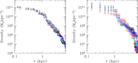
Figure 2: Gravitational mass density distributions over radius, obtained from runs done with data drawn from three different phase space distributions ($f_{Gauss},\>f_{WD}\>f_{Michie}$) that are distinguished from each other in terms of the inherent degree of anisotropy in their forms. $\rho(r)$ estimated from run performed with data $S_{isotropy}$ is in black, with $S_{WD}$ is in red and with $S_{Michie}$ is in blue. The $\rho(r)$ implied by the fiduciary test potential $\Phi_{test}(r)$ is in cyan. The left panel displays results obtained when the constraint of total mass is included ($M_{0}\approx 4.06\times 10^{11}$ M_⊙ within about 8.7 kpc). On the right, the general inconsistency between the estimated profiles, when the mass constraint is excluded, is brought out.

The total mass constraint is expected to narrow down the range of solutions possible; in this sense it acts as a prior on the solution for $\rho(\cdot)$. We test if the chosen data samples, when input into CHASSIS, recover a $\Phi(r)$ that is concurrent with $\Phi_{test}(r)$ when we include/exclude the constraint that total mass within $r=R_{E}$ is $M_{0}$. Here $M_{0}$ is obtained from literature as about 4.06$\times 10^{11}$ M_⊙, with errors of $\delta M_{0}=\pm 0.2\times 10^{11}$ M_⊙ and $R_{E}\approx$8.7 kpc (Koopmans $\&$ Treu 2003). We incorporate the constraint by adding a penalty function to the definition of the likelihood; the role of this penalty function is to penalise any solution that implies a total gravitational mass within $R_{E}$ ($M_{c}(R_{E})$) different from $M_{0}$. This penalty function is $\alpha|M_{c}(R_{E})-M_{0}|/2\delta M_{0}$. Here $\alpha$ is a flag, designed to include or exclude the constraint from the definition of the likelihood, depending on whether it is 1 or 0 respectively.

The results of conducting our test runs are shown in Figure 2. We find that when the constraint is included, the $\rho(r)$ profiles are consistent with each other within errors, irrespective of the anisotropy in the data used to obtain this profile. In absence of guidance from the constraint, anisotropy affects results.

6 Summary

Here we have discussed the novel nonparametric Bayesian algorithm CHASSIS that estimates the most likely phase space $pdf$ ($f(\cdot)$) from which an observed sample of 1-D component of velocities of individual galactic members is drawn, at the most likely gravitational potential $\Phi(\cdot)$ of the galaxy. The main purpose of this paper is to bring out the fact that CHASSIS is a robust and viable algorithm that can be implemented to extract the all-important gravitational matter density distribution in distant galaxies, even within the domain of very sparse and incomplete data. Given the dearth of measurements in these systems, it is prudent to work with a small number of degrees of freedom. With this in mind, one version of CHASSIS has been designed to work under the purview of the assumption of isotropy in phase space, by which we imply an $f(\cdot)$ that is symmetric in the 3 velocity and 3 spatial coordinates. In another version, the assumption of isotropy is not made and CHASSIS is made to work with a greater number of dof (Chakrabarty $\&$ Saha, under preparation).

We offer independent means of tackling the obvious fallout of the assumption of isotropy, when invoked; phase space $pdf$s from which realistic data are drawn, will not be isotropic in general, leading to spurious solutions for $f(\cdot)$ and $\Phi(\cdot)$. Firstly, a robust test of hypothesis is developed that tests the assumption of isotropy, given the data. This test is modelled after Pereira $\&$ Stern’s (1999) FBST and is designed to work in the nonparametric context. Data available in astrophysical literature are implemented to conclude that kinematic data of distinct galactic member populations will in general provide distinct gravitational mass distributions. The multistability of the example galaxy is demonstrated and the folly of this mode of mass determination is indicated. Secondly, we demonstrate that the usage of information about total gravitational mass, available in the literature, can constrain the sought gravitational matter density distribution, irrespective of anisotropy in the data. Such a constraint basically supplements for the uninformative priors that we use within CHASSIS.

Currently, we are working on the establishment of a critical value of the evidence value in favour of a given null. This will enable the quantified judgement of when to reject or accept the null, given the data. At the moment, our implementation of FBST only allows for a comparative judgement.

References

- [1]
- [2] Gelman, A. Rubin, D. B.1992, Statistical Science, 7, 457.
- [3] Hastings, W. K., 1970, Biometrika, 57, 97.
- [4] Chib, S. Greenberg, E. 1995, American Statistician, 49, 327.
- [5] Metropolis, N., Rosenbluth, A. W., Rosenbluth, M. N., Teller, A., Teller, H. 1953, Jl. of Chemical Physics, 21, 1087.
- [6] Dubrovin, B. A., Fomenko, A. T. & Novikov, S. P. 1990 Modern Geometry: Methods and Applications, pg. 314.
- [7] Chakrabarty, D. & Portegies Zwart, S. 2004, Astronomical Jl., 128, 1046.
- [8] Chakrabarty, D. & Saha, P. 2001, Astronomical Jl., 122, 232.
- [9] Bissantz, N., & Munk, A. 2001, Astronomy Astrophysics, 376, 735.
- [10] Koopmans, L. V. E., & Treu, T. 2003, Astrophysical Jl., 583, 606.
- [11] Madruga, R. M., Esteves, L. G. Wechsler, S., 2001 Test, 10, 291.
- [12] Pereira, C. A. de B., Stern, J. M. Wechsler, S., 2008, Bayesian Analysis, 3, 79.
- [13] Pereira, C. A. de B. Stern, J.M., 1999, Entropy, 1, 99.
- [14] Douglas, N. G., Napolitano, N. R., Romanowsky, A. J., Coccato, L., Kuijken, K., Merrifield, M. R., Arnaboldi, M., Gerhard, O., Freeman, K. C., Merrett, H. R., Noordermeer, E. Capaccioli, M., 2007, Astrophysical Jl., 664, 257.
- [15] Bergond, G., Zepf, S. E., Romanowsky, A. J., Sharples, R. M., & Rhode, K. L., 2006, Astronomy Astrophysics, 448, 155.
- [16]