RUB-TPII-07/09
Pion form factor in the QCD sum-rule approach
with nonlocal condensates

Abstract

We present results of a calculation of the electromagnetic pion form factor within the framework of QCD Sum Rules with nonlocal condensates, using a perturbative spectral density which includes $O(\alpha_{s})$ contributions.

1 Introduction

The pion—its distribution amplitude and form factor—stands tall as a role model for the modern description of hadrons in terms of quarks and gluons within QCD. At high momenta $Q^{2}$, the pion form factor can be written as a convolution $F_{\pi}(Q^{2})=\varphi_{\pi}^{\text{out}}\otimes T(Q^{2})\otimes\varphi_{\pi}^{\text{in}}$ on account of the factorization theorem, where the symbol $\otimes$ means an integration over the longitudinal momenta of the quark and antiquark in the pion state factorized at some scale $\mu^{2}$. All binding effects due to the nonperturbative color dynamics are absorbed into the pion distribution amplitudes $\varphi_{\pi}^{\text{in}}$ for the incoming and $\varphi_{\pi}^{\text{out}}$ for the outgoing pion. However, at low and intermediate momenta $Q^{2}$ this factorization procedure becomes inapplicable because the long-range interactions cannot be separated into factorizing pion distribution amplitudes $\varphi_{\pi}$, as above, so that the convolution approach is not very reliable.

In a recent paper [1], we have proposed a different theoretical framework for the calculation of the pion form factor, which is based on QCD sum rules with nonlocal condensates (NLC) [2, 3, 4], employing an Axial-Axial-Vector (AAV) correlator. Suffice it to say here that our scheme differs from previous ones in several respects that will be considered in the next section. A prolegomenon of the results we derived (see Sec. 3): the proposed method yields predictions for the spacelike pion form factor that compare well with the data in that momentum region which is currently accessible to measurements, covering also the range of momenta to be probed by the 12 GeV upgraded CEBAF accelerator at JLab. Our conclusions are summarized in Sec. 4.

2 Three-point QCD sum rule for the pion form factor

Let us make here a second, more detailed pass, on some of the topics briefly mentioned in the Introduction, recalling the AAV correlator

$$\int\!\!\!\!\int\!\!d^{4}x\,d^{4}y\,e^{i(qx-p_{2}y)}\langle 0|T\!\left[J^{+}_{5\beta}(y)J^{\mu}(x)J_{5\alpha}(0)\right]\!|0\rangle\,,$$ (1)

where $q$ denotes the photon momentum ($q^{2}=-Q^{2}$) and $p_{2}$ is the outgoing pion momentum. The quantities $J^{\mu}(x)=e_{u}\,\overline{u}(x)\gamma^{\mu}u(x)+e_{d}\overline{d}(x)\gamma^{\mu}d(x)$ and $J_{5\alpha}(x)=\overline{d}(x)\gamma_{5}\gamma_{\alpha}u(x)$, $J^{+}_{5\beta}(x)=\overline{u}(x)\gamma_{5}\gamma_{\beta}d(x)$ are the electromagnetic current and the axial-vector currents, respectively, where $e_{u}=2/3$ and $e_{d}=-1/3$ stand for the electric charges of the $u$ and the $d$ quarks. Referring for further details to [5, 6] for the case of local condensates and to [4] for nonlocal ones, we proceed by writing down the sum rule we will employ:

$$f_{\pi}^{2}\,F_{\pi}(Q^{2}) = \int\limits_{0}^{s_{0}}\!\!\int\limits_{0}^{s_{0}}\!ds_{1}\,ds_{2}\ \rho_{3}(s_{1},s_{2},Q^{2})\,e^{-(s_{1}+s_{2})/M^{2}}$$ (2)

$$+\Phi_{\text{G}}(Q^{2},M^{2})+\Phi_{\langle\bar{q}q\rangle}(Q^{2},M^{2})\,.$$

Note that the quark-condensate contribution

$$\Phi_{\langle\bar{q}q\rangle}(Q^{2},M^{2})=\Phi_{\text{4Q}}(Q^{2},M^{2})+\Phi_{\text{2V}}(Q^{2},M^{2})+\Phi_{\bar{q}Aq}(Q^{2},M^{2})$$ (3)

contains the four-quark condensate (4Q), the bilocal vector-quark condensate (2V), and the antiquark-gluon-quark condensate ($\bar{q}Aq$), while the term $\Phi_{\text{G}}(Q^{2},M^{2})$ represents the gluon-condensate contribution to the sum rule. The crucial quantity in the sum rule is the three-point spectral density

$$\rho^{(1)}_{3}(s_{1},s_{2},Q^{2}) = \left[\rho_{3}^{(0)}(s_{1},s_{2},Q^{2})+\frac{\alpha_{s}(Q^{2})}{4\pi}\,\Delta\rho_{3}^{(1)}(s_{1},s_{2},Q^{2})\right]\,.$$ (4)

The leading-order spectral density has been calculated long ago [5, 6], whereas the analogous next-to-leading order (NLO) version $\Delta\rho_{3}^{(1)}(s_{1},s_{2},Q^{2})$ has been derived recently in [7]. The contribution from higher resonances is usually taken into account in the form

$$\rho_{\text{HR}}(s_{1},s_{2})=\left[1-\theta(s_{1}<s_{0})\theta(s_{2}<s_{0})\right]\,\rho_{3}(s_{1},s_{2},Q^{2})$$ (5)

and contains the continuum threshold parameter $s_{0}$. In the investigation [1], reported upon here, we use in the perturbative spectral density a version of the running coupling that avoids Landau singularities by construction (see for reviews in [8, 9, 10]). At the one-loop level, one has [8]

$$\alpha_{s}(Q^{2}) = \frac{4\pi}{b_{0}}\left(\frac{1}{\ln(Q^{2}/\Lambda_{\text{QCD}}^{2})}-\frac{\Lambda_{\text{QCD}}^{2}}{Q^{2}-\Lambda_{\text{QCD}}^{2}}\right)$$ (6)

with $b_{0}=9$ and $\Lambda_{\text{QCD}}=300$ MeV.

The key elements of our analysis are these: (i) All interquark distances in the quark-gluon-antiquark condensate are nonlocal and the nonlocality is parameterized via the quark-virtuality parameter $\lambda_{q}^{2}$ [2] with the value 0.4 GeV². (ii) A modified Gaussian model for the nonlocal condensate is used, recently proposed in [11], and the prediction for $F_{\pi}$ is compared with the results derived in [12], obtained by using the minimal Gaussian model [3, 13, 14], and from other theoretical models [15, 16] as well. The virtue of the modified NLC model is that it helps minimizing the transversality violation of the two-point correlator of vector currents. (iii) A spectral density is used that includes terms of $O(\alpha_{s})$, i.e., NLO perturbative contributions. Moreover, the coupling entering the spectral density is analytic, as stated above, so that the calculation of the pion form factor is not influenced by the Landau pole. It was shown in [17, 12] that the Landau pole can obscure the predictions for the pion form factor even at momentum values much larger than $\Lambda_{\text{QCD}}$.

3 Predictions

Using the presented scheme, we obtain predictions for the pion form factor [1], which are shown in Fig. 1. Our results are presented in the form of shaded bands, the aim being to include the inherent theoretical uncertainties of the method. The band contained within the solid lines gives the predictions we obtained with the improved Gaussian NLC model, whereas the corresponding findings from the minimal NLC model are shown in the band with the dashed boundaries. The central curves in each band (illustrated by a thick solid and a thick dashed line) are interpolation formulas, whose explicit form can be found in [1]. For the understanding of these predictions it is instructive to remark that our method provides results that remain valid—though with reduced accuracy—even at higher values of the momentum up to $Q^{2}\approx 10$ GeV².

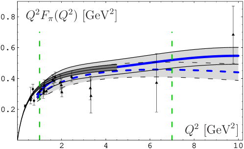
Figure 1: Scaled pion form factor $Q^{2}F_{\pi}(Q^{2})$ for the minimal (dashed blue lines) and the improved (solid blue lines) NLC model using $\lambda_{q}^{2}=0.4$ GeV² in comparison with experimental data of the Cornell [18] (triangles) and the JLab Collaboration [19] (diamonds). The shaded band within dashed lines shows the minimal model, whereas the variance of the improved model is indicated by solid lines. The lattice result of [20] is also shown as a dark-grey strip. The two broken vertical lines mark the region, where the influence of the particular Gaussian NLC model used is not severe.

Let us now discuss some technical details. The value of $s_{0}(Q^{2})$ at a given value of $Q^{2}$ is determined by demanding minimal sensitivity of $F_{\pi}(M^{2},s_{0})$ on the Borel parameter $M^{2}$ in the fiducial interval of the SR. These intervals $M^{2}\in[M^{2}_{-}/2,M^{2}_{+}/2]$ are determined from the corresponding two-point NLC QCD SR and turn out to be $M^{2}_{-}=1$ GeV², $M^{2}_{+}=1.7$ GeV² for the minimal NLC model and $M^{2}_{-}=1$ GeV², $M^{2}_{+}=1.9$ GeV² for the improved NLC model, while the associated values of the pion decay constant read $f_{\pi}=0.137$ GeV² and $f_{\pi}=0.142$ GeV², respectively. Notice that the value of the Borel parameter $M^{2}$ in the three-point SR roughly corresponds to the Borel parameter in the two-point SR, having, however, twice its magnitude. A stable window for the Borel parameter is obtained for thresholds in the range between 0.65 and 0.85 GeV² [1]. As a rule, the higher the value of $s_{0}$, the larger the form factor because the perturbative input increases. The sensitivity of the obtained form-factor predictions on the particular NLC model employed is rather weak in the region of momenta delimited in Fig. 1 by two vertical broken lines. We close this discussion by remarking that the overall agreement between the obtained predictions and the available experimental data from [18, 19] is rather good. Moreover, they comply with the recent lattice calculation of [20], which is shown in the same figure in terms of a dark-grey strip, bounded from high-$Q^{2}$ values at $Q^{2}\simeq 4$ GeV².

In Fig. 2, we compare our predictions with other theoretical results, derived from the AdS/QCD correspondence (so-called holographic QCD), and some other models (including also the experimental data). As in the previous figure, the shaded bands show our predictions for the minimal (dashed lines) and the improved NLC model (solid lines). The dashed (red) line at low-$Q^{2}$ (terminating at about 4 GeV²) represents the prediction derived in [5] from QCD SR, while the thicker broken line below all other curves is the result of a calculation [21] based on Local Duality QCD SR. The predictions from AdS/QCD are denoted by the upper short-dashed (green) line—soft-wall model [15]—and the penultimate dash-dot-dotted (green) line, obtained with a Hirn–Sanz-type holographic model [16]. The LD result of [21] is shown as a dash-dotted (red) line.

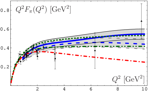
Figure 2: Scaled pion form factor $Q^{2}F_{\pi}(Q^{2})$ within a band including uncertainties for the minimal (dashed lines) and the improved (solid lines) NLC model, using in both cases $\lambda_{q}^{2}=0.4$ GeV². The experimental data are as in Fig. 1. The predictions from AdS/QCD are: upper short-dashed (green) line—soft-wall model [15]; dash-dot-dotted (green) line—Hirn–Sanz-type holographic model [16]. The dash-dotted (red) line corresponds to the LD result of [21].

4 Conclusions

Here we have studied a three-point AAV correlator within the QCD sum-rule approach with nonlocal condensates in order to obtain predictions for the spacelike pion form factor pertaining to that momentum region accessible to experiment at present and in the near future. The full-fledged analysis can be found in [1], where we also included in our discussion the so-called Local-Duality approach [5].

The principal ingredients of our approach are a spectral density that includes $O(\alpha_{s})$ corrections, whereas the coupling used has an analytic structure without Landau singularities, and an improved Gaussian ansatz for the nonlocal condensate. Our findings are supported by both the existing experimental data and also a recent lattice calculation in the momentum range up to approximately 10 GeV².

References

- [1] A. P. Bakulev, A. V. Pimikov, and N. G. Stefanis, Phys. Rev. D79, 093010 (2009).
- [2] S. V. Mikhailov and A. V. Radyushkin, JETP Lett. 43, 712 (1986).
- [3] S. V. Mikhailov and A. V. Radyushkin, Phys. Rev. D45, 1754 (1992).
- [4] A. P. Bakulev and A. V. Radyushkin, Phys. Lett. B271, 223 (1991).
- [5] V. A. Nesterenko and A. V. Radyushkin, Phys. Lett. B115, 410 (1982).
- [6] B. L. Ioffe and A. V. Smilga, Phys. Lett. B114, 353 (1982).
- [7] V. V. Braguta and A. I. Onishchenko, Phys. Lett. B591, 267 (2004).
- [8] D. V. Shirkov and I. L. Solovtsov, Phys. Rev. Lett. 79, 1209 (1997); Theor. Math. Phys. 150, 132 (2007).
- [9] A. P. Bakulev, Phys. Part. Nucl. 40, 715 (2009).
- [10] N. G. Stefanis, arXiv:0902.4805 [hep-ph].
- [11] A. P. Bakulev and A. V. Pimikov, PEPAN Lett. 4, 637 (2007).
- [12] A. P. Bakulev, K. Passek-Kumerički, W. Schroers, and N. G. Stefanis, Phys. Rev. D70, 033014 (2004); D70, 079906(E) (2004).
- [13] A. P. Bakulev and S. V. Mikhailov, Phys. Lett. B436, 351 (1998).
- [14] A. P. Bakulev, S. V. Mikhailov, and N. G. Stefanis, Phys. Lett. B508, 279 (2001).
- [15] S. J. Brodsky and G. F. de Teramond, Phys. Rev. D77, 056007 (2008).
- [16] H. R. Grigoryan and A. V. Radyushkin, Phys. Rev. D78, 115008 (2008).
- [17] N. G. Stefanis, W. Schroers, and H.-C. Kim, Phys. Lett. B449, 299 (1999); Eur. Phys. J. C18, 137 (2000).
- [18] C. J. Bebek et al., Phys. Rev. D9, 1229 (1974); D13, 25 (1976); D17, 1693 (1978).
- [19] G. M. Huber et al., Phys. Rev. C78, 045203 (2008).
- [20] D. Brommel et al., Eur. Phys. J. C51, 335 (2007).
- [21] V. Braguta, W. Lucha, and D. Melikhov, Phys. Lett. B661, 354 (2008).