Avoid the Tsunami of the Dirac sea in the Imaginary Time Step method

Abstract

The discrete single-particle spectra in both the Fermi and Dirac sea have been calculated by the imaginary time step (ITS) method for the Schrödinger-like equation after avoiding the ”tsunami” of the Dirac sea, i.e., the diving behavior of the single-particle level into the Dirac sea in the direct application of the ITS method for the Dirac equation. It is found that by the transform from the Dirac equation to the Schrödinger-like equation, the single-particle spectra, which extend from the positive to the negative infinity, can be separately obtained by the ITS evolution in either the Fermi sea or the Dirac sea. Identical results with those in the conventional shooting method have been obtained via the ITS evolution for the equivalent Schrödinger-like equation, which demonstrates the feasibility, practicality and reliability of the present algorithm and dispels the doubts on the ITS method in the relativistic system.

The imaginary time step (ITS) method ev8-80 , which searches for the direction of the steepest descent of energy and follows it in iterative steps until the local minimum on the energy surface is reached, is an effective approach to solve the non-relativistic problems in coordinate space and has achieved lots of success in the conventional mean field ev8-cpc05 . As noted already in Ref. ev8-80 , since only the lowest eigenstate is reached after several exponential transformations, the method is applied to the single-particle Hamiltonians of which the spectrum is bounded from below.

From the physics point of view, a lot of novel aspects of nuclear structure and entirely unexpected features have been found in the ”exotic nuclei” Tanihata85 ; RIB01 ; Jonson04 ; Jensen04 . The extreme neutron richness of exotic nuclei and the physics related to the low density in the tails of matter distributions have not only attracted attention in nuclear physics and astrophysics but also provided a challenge to solve complex many-body problem in coordinate space.

As one of the best candidates for the description of exotic nuclei, the Relativistic Mean Field approach Serot86 has achieved lots of success in describing many nuclear phenomena during the past years Ring96 ; Vretenar05 ; MengPPNP .

Subsequently, the Relativistic Continuum Hartree-Bogoliubov (RCHB) theory MengHaloPRL provides a fully self-consistent treatment of pairing correlations in the presence of the continuum and thus a reliable description of nuclei far away from the line of $\beta$-stability, which well reproduced the halo phenomena in ¹¹Li. A natural extension of the RCHB theory is the exploration of deformed exotic nuclei and to pin down the existence of deformed halo. Efforts along this line have been made in the past several years. Due to the difficulty in solving the coupled channel differential equations for deformed system in coordinate space Price87 , the method for expansion in Woods-Saxon basis was proposed ZhouWS03 , which becomes very time consuming for the heavy system.

For the ITS method, the extension from spherical to deformed systems is straightforward. However, whether the ITS method can be applied for the relativistic system still remains an interesting question due to the existence of the Dirac sea. Although, by implementing the effective Hamiltonian deduced for the upper component to the existing ITS routine for the Skyrme-Hartree-Fock approach, efforts have been made to get the single-particle levels in the Fermi sea, e.g., in Ref. Gogelein07 , further works are still necessary to justify its feasibility and reliability, and to understand the influence of the Dirac sea explicitly.

In this paper, the ITS method will be applied to solve the Dirac equation in coordinate space. The disaster of the Dirac sea confronted in the direct application of the ITS method for the Dirac equation will be analyzed and discussed in detail. Reliable and practical recipe to avoid the disaster will be provided by examining the relation between the Dirac equation and its ”equivalent” Schrödinger-like equation.

The main idea and detailed formalism of the ITS method can be found in Ref. ev8-80 . The ITS evolution of the single-particle wave functions reads

$$\left|\Psi_{a}^{(n+1)}\right\rangle={\left(1-\lambda\hat{h}\right)}\left|\varphi_{a}^{(n)}\right\rangle,\quad\lambda\equiv\Delta t/\hbar,$$ (1)

where the exponential series is truncated at the first order as in Ref. ev8-cpc05 , $\hat{h}$ is the single-particle Hamiltonian and {$\varphi_{a}^{(n)}$} is a set of orthogonal single-particle wave functions at time $t_{n}=n\Delta t$. Orthonormalizing {$\Psi_{a}^{(n+1)}$} thus obtained generates a new set of orthogonal wave functions {$\varphi_{a}^{(n+1)}$} which will be used for the next ITS evolution. The total energy of the system will decrease as the time evolves, until it finds a local minimum on the energy surface. The corresponding wave functions {$\varphi_{a}$} will simultaneously converge to the eigenstates of the single-particle Hamiltonian $\hat{h}$.

The ITS method has been successfully implemented in the conventional mean field approach. For the relativistic case, the main issue is to solve the Dirac equation,

$$\left\{\mbox{\boldmath$\alpha$}\cdot\mbox{\boldmath$p$}+\beta\left[M+S(\mbox{\boldmath$r$})\right]+V(\mbox{\boldmath$r$})\right\}\varphi_{a}=(\varepsilon_{a}+M)\varphi_{a},$$ (2)

with the scalar and vector potentials $S(\mbox{\boldmath$r$})$ and $V(\mbox{\boldmath$r$})$. For clarity and simplicity, $V(\mbox{\boldmath$r$})\pm S(\mbox{\boldmath$r$})$ are assumed to be the spherical Woods-Saxon potentials similar as in Ref. ZhouWS03 , then the Dirac spinor takes the form,

$$\varphi_{a}=\displaystyle\frac{1}{r}\left(\begin{array}[]{c}iF_{a}(r)\mathcal{Y}_{a}(\hat{\mbox{\boldmath$r$}})\\ G_{a}(r)\hat{\sigma}_{r}\mathcal{Y}_{a}(\hat{\mbox{\boldmath$r$}})\end{array}\right)\chi_{\frac{1}{2}}(q_{a}),$$ (3)

with the isospinor $\chi_{\frac{1}{2}}(q_{a})$, and the spherical spinor $\mathcal{Y}_{a}(\hat{\mbox{\boldmath$r$}})$. Throughout this paper, the single-particle state in either Fermi or Dirac sea is labeled by the quantum numbers $\{n_{a},l_{a},\kappa_{a},j_{a}\}$ of the upper component, where $\kappa_{a}=\pm|j_{a}+1/2|$ for $l_{a}=j_{a}\pm 1/2$. The radial Dirac equation for $F_{a}$ and $G_{a}$ can thus be obtained as

$$\left(\begin{array}[]{cc}V+S&\displaystyle-\frac{d}{dr}+\frac{\kappa_{a}}{r}\\ \displaystyle\frac{d}{dr}+\frac{\kappa_{a}}{r}&V-S-2M\end{array}\right)\left(\begin{array}[]{c}F_{a}(r)\\ G_{a}(r)\end{array}\right)=\varepsilon_{a}\left(\begin{array}[]{c}F_{a}(r)\\ G_{a}(r)\end{array}\right),$$ (4)

in which the $2\times 2$ matrix operator on the l.h.s. is the single-particle Hamiltonian $\hat{h}$ to be used in Eq. (1) for the ITS evolution.

For the initial orthogonal wave functions {$\varphi_{a}^{(1)}$}, the upper components are taken as spherical Bessel function and the lower components are assumed to be zero. The first(second)-order differential operator in the single-particle Hamiltonian is calculated by the seven(nine)-points formula as in Ref. ev8-cpc05 . The ITS evolution is carried out in coordinate space within a spherical box $[0,R]$ with the mesh size $dr=0.1\sim 0.5$ fm and a typical time step $\Delta t=10^{-26}$ s.

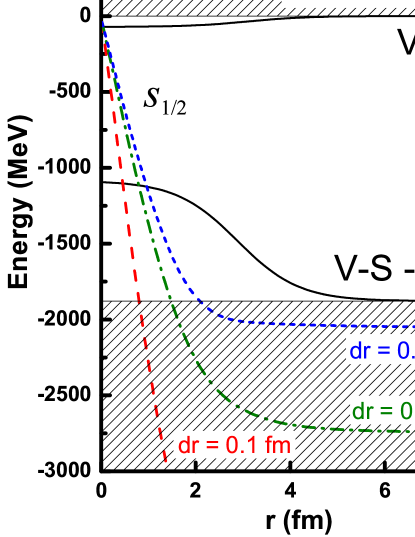
Figure 1: (color online) Disaster for solving the Dirac equation with scalar and vector Woods-Saxon potentials in the ITS method. Taking ¹⁶O as an example, the diving behaviors into the Dirac sea during the ITS evolution are shown for the neutron single-particle level $s_{1/2}$, which is evolved in a spherical box with $R=20$ fm, and mesh sizes $dr=0.5$ fm (short-dashed line), $0.2$ fm (dash-dotted line), and $0.1$ fm (dashed line) respectively. The shaded areas are the continuum in the Fermi and Dirac sea.

Taking the Woods-Saxon potentials for $V(\mbox{\boldmath$r$})\pm S(\mbox{\boldmath$r$})$ corresponding to ¹⁶O as an example, the ITS evolutions of the lowest $s_{1/2}$ orbital for neutron are shown in Fig. 1. It is found that although the initial state is set in the Fermi sea, the single-particle energy will inevitably dive into the Dirac sea as the time evolves. This is not surprising. Because the ITS method searches for the states with the lowest energy in the whole spectra, the single-particle energy should dive to the negative infinity corresponding to the wave function with infinite nodes. In practice, however, as the node number is limited by the given box and mesh sizes, one can always achieve convergence for the ITS evolution. The convergent single-particle energy will dive deeper in the Dirac sea for smaller mesh size.

One may wonder whether the ITS evolution is able to produce any $s_{1/2}$ orbital outside the Dirac sea. Attempts have been made but a dilemma has been found. As indicated in Fig. 1, if one takes a large mesh size, the lowest $s_{1/2}$ orbital may lie shallow in the Dirac sea, and the whole spectrum is sparse. Taking a box with $R=10$ fm and $dr=0.5$ fm as an example, a survivor $2s_{1/2}$ is found in the discrete region of the Dirac sea, and is compared with the ”exact” results obtained by the shooting method MengPPNP with $R=20$ fm and $dr=0.1$ fm in Fig. 2. Its single-particle energy and radial wave functions are in good agreement with the ”exact” ones, which shows that at least some physical solutions in the Dirac sea are accessible by the direct ITS evolution for the Dirac equation. However, it is at a cost of precision, and it is gloomy to go beyond the Dirac sea. To calculate more single-particle states, one should take smaller mesh size or larger box, which determines the number of orthogonal wave functions. However, the whole spectrum of $s_{1/2}$ orbitals becomes denser and dives deeper, thus it is incurable to go beyond the Dirac sea.

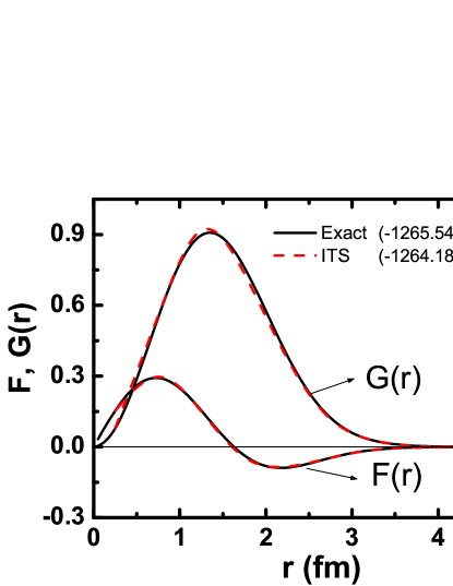
Figure 2: (color online) Neutron radial wave functions and single-particle energy for the survivor $2s_{1/2}$ in the disaster of the Dirac sea. The ITS evolution for the Dirac equation is performed in a spherical box with $R=10$ fm and $dr=0.5$ fm, while the ”exact” results are obtained by the shooting method with $R=20$ fm and $dr=0.1$ fm.

Therefore, this is indeed a great disaster to perform the ITS evolution directly for the Dirac equation, since physical solutions are completely submerged by the mighty flood with negative energy states, or the ”tsunami” of the Dirac sea.

In order to avoid the ”tsunami”, one possibility is to perform the ITS evolution for the Schrödinger-like equation instead of the Dirac equation. Naively, such possibility might be doubted as the Schrödinger-like equation is deduced from the Dirac equation, and they are equivalent in the sense that all the solutions of the Dirac equation satisfy the corresponding Schrödinger-like equation. However, they are not equivalent in the sense discussed below.

From Eq. (4), the relation between the upper and lower components can be obtained as,

$$G_{a}=\frac{1}{2M_{+}}\left(\frac{dF_{a}}{dr}+\frac{\kappa_{a}}{r}F_{a}\right),$$ (5)

with the effective mass $M_{+}=M+(S-V+\varepsilon_{a})/2$, and the corresponding Schrödinger-like equation for the upper component is $\hat{h}F_{a}=\varepsilon_{a}F_{a}$, with the effective Hamiltonian,

$$\hat{h}=-\frac{1}{2M_{+}}\frac{d^{2}}{dr^{2}}+\frac{1}{2M_{+}^{2}}\frac{dM_{+}}{dr}\frac{d}{dr}+\left[(V+S)+\frac{1}{2M_{+}^{2}}\frac{dM_{+}}{dr}\frac{\kappa_{a}}{r}+\frac{1}{2M_{+}}\frac{\kappa_{a}(\kappa_{a}+1)}{r^{2}}\right].$$ (6)

Now the difference between the Dirac equation and the corresponding Schrödinger-like equation is clear. For the Dirac equation, the single-particle spectra extend from the positive to the negative infinity. While for the Schrödinger-like equation, although the effective Hamiltonian in Eq. (6) which contains the single-particle energy is quite sophisticated, it can be reduced as $\hat{h}=\displaystyle\frac{P^{2}}{2M_{+}(\varepsilon_{a})}+U(\varepsilon_{a})$. Therefore, with the trial single-particle energy $\varepsilon_{a}$ in the Fermi sea, the positive definite effective mass will ensure that $\varepsilon_{a}\geq U(\varepsilon_{a})$. As a result, the single-particle spectrum in the Fermi sea can be separated from that in the Dirac sea, and then the ITS evolution could be applied for the Schrödinger-like equation to obtain the solutions in the Fermi sea. Furthermore, in order to obtain the solutions in the Dirac sea, one could apply the similar technique to perform the ITS evolution for the charge conjugated Schrödinger-like equation. Therefore, it is the transform from the Dirac equation to the Schrödinger-like equation that allows the ITS evolution for the single-particle spectra in either the Fermi sea or the Dirac sea, and thus provides a ”life buoy” to avoid the disaster of the Dirac sea.

Using the effective Hamiltonian in Eq. (6), the upper component is obtained by the ITS evolution for the Schrödinger-like equation. The corresponding lower component is obtained by Eq. (5). Then the Dirac spinor including both the upper and lower components are orthonormalized for the next iteration.

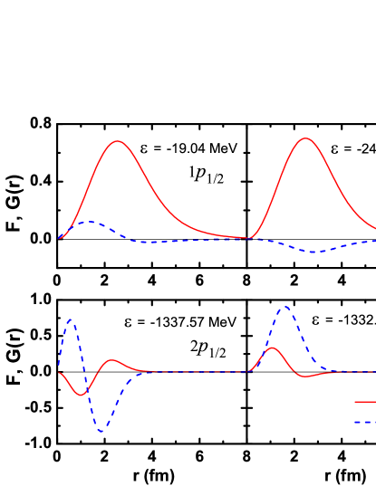
Figure 3: (color online) Neutron radial wave functions and single-particle energies for $1p$ spin doublets in the Fermi sea (upper panels) and $2p$ spin doublets in the Dirac sea (lower panels) obtained by the ITS evolution for the Schrödinger-like equation with $R=20$ fm and $dr=0.1$ fm.

As examples, the neutron radial wave functions and single-particle energies for $1p$ spin doublets in the Fermi sea and $2p$ spin doublets in the Dirac sea obtained by the ITS evolution for the Schrödinger-like equation with $R=20$ fm and $dr=0.1$ fm are respectively given in the upper and lower panels in Fig. 3. Both the wave functions and single-particle energies are identical with the ”exact” results obtained by the shooting method.

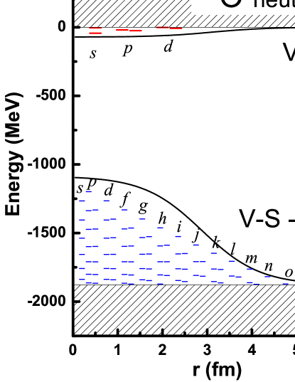
Figure 4: (color online) Neutron discrete single-particle spectra of ¹⁶O in the Fermi and Dirac sea obtained after avoiding the disaster of the Dirac sea via the ITS evolution for the Schrödinger-like equation. For each pair of the spin doublets, the left (right) is for $\kappa>0$ ($<0$).

Similarly, all the discrete single-particle spectra identical with the ”exact” ones for neutron of ¹⁶O in both the Fermi and Dirac sea are obtained as shown in Fig. 4. The spin doublets are presented in pairs, with the left (right) one is for $\kappa>0~{}(<0)$. It should be noted that the single-particle states are always labeled by the quantum numbers of the upper component, different from those in Ref. ZhouPRL03 . Therefore, it is clearly shown that the disaster of the Dirac sea can be avoided via the ITS evolution for the equivalent Schrödinger-like equation.

In conclusion, the discrete single-particle spectra in both the Fermi and Dirac sea have been calculated by the ITS evolution for the Schrödinger-like equation after avoiding the ”tsunami” of the Dirac sea.

The ITS method, which has been widely used in the conventional mean field approaches, will inevitably meet a serious challenge when it is directly applied for the Dirac equation. All the single-particle levels will dive into the Dirac sea during the ITS evolution, and the physical solutions of the Dirac equation are submerged by the ”tsunami” of the Dirac sea. Fortunately, the Schrödinger-like equation deduced from the Dirac equation provides the life buoy to survive the ”tsunami”. For a long time, the Schrödinger-like equation was generally regarded to be equivalent to the Dirac equation. However, by the transform from the Dirac equation to the Schrödinger-like equation, the single-particle spectra, which extend from the positive to the negative infinity, can be separately obtained by the ITS evolution in either the Fermi sea or the Dirac sea. The ITS evolution for the Schrödinger-like or charge conjugated Schrödinger-like equation will provide the solution in the Fermi or Dirac sea, which are identical with the ”exact” ones obtained by the shooting method.

The successful implementation here fully demonstrated the feasibility, practicality and reliability for the ITS method in the relativistic system.

References

- (1) K. T. R. Davies, H. Flocard, S. Krieger, and M. S. Weiss, Nucl. Phys. A 342, 111 (1980).
- (2) P. Bonche, H. Flocard, and P. H. Heenen, Com. Phys. Com. 171, 49 (2005).
- (3) I. Tanihata et al., Phys. Rev. Lett. 55, 2676 (1985).
- (4) C. A. Bertulani, M. S. Hussein, and G. Münzengerg, Physics of Radioactive Beams, Nova Science Publishers, Inc., (2001).
- (5) B. Jonson, Phys. Rep. 389, 1 (2004).
- (6) A. S. Jensen, K. Riisager, D. V. Fedorov, E. Garrido, Rev. Mod. Phys. 76, 215 (2004).
- (7) B. D. Serot and J. D. Walecka, Adv. Nucl. Phys. 16, 1 (1986).
- (8) P. Ring, Prog. Part. Nucl. Phys. 37, 193 (1996).
- (9) D. Vretenar, A. V. Afanasjev, G. A. Lalazissis, and P. Ring, Phys. Rep. 409, 101 (2005).
- (10) J. Meng, H. Toki, S. G. Zhou, S. Q. Zhang, W. H. Long, and L. S. Geng, Prog. Part. Nucl. Phys. 57, 470 (2006).
- (11) J. Meng and P. Ring, Phys. Rev. Lett. 77, 3963 (1996).
- (12) C. E. Price and G. E. Walker, Phys. Rev. C 36, 354 (1987).
- (13) S. G. Zhou, J. Meng and P. Ring, Phys. Rev. C 68, 034323 (2003).
- (14) P. Gögelein and H. Müther, Phys. Rev. C 76, 024312 (2007).
- (15) S. G. Zhou, J. Meng, and P. Ring, Phys. Rev. Lett. 91, 262501 (2003).