Multiple Interactions, Saturation, and Final States in $pp$ Collisions and DIS

Abstract

Dedicated to the memory of Jan Kwieciński

In high energy collisions saturation and multiple collisions are most easily accounted for in transverse coordinate space, while analyses in momentum space have been more suitable for calculating properties of exclusive final states. In this talk I describe an extension of Mueller’s dipole cascade model, which attempts to combine the good features of both these descriptions. Besides saturation it also includes effects of correlations and fluctuations, which have been difficult to account for in previous approaches. The model reproduces successfully total, elastic, and diffractive cross sections in $pp$ collisions and DIS, and a description of final states will be ready soon.

12.38-t, 13.60.Hb, 13.85-t

1 Introduction

In this talk I want to discuss some results related to saturation and multiple collisions obtained in collaboration with Emil Avsar, Christoffer Flensburg, and Leif Lönnblad [1, 2]. In high energy $pp$ collisions the minijet cross section is much larger than the total cross section. This implies that each event contains on average more than one minijet pair, and multiple subcollisions are an essential feature of high energy hadronic reactions. A formulation in transverse coordinate space and the eikonal approximation are particularly suited for a treatment of these features, and has been successfully applied to $\gamma^{*}p$ collisions, both for total and diffractive scattering cross sections [3, 4].

The application of the eikonal formalism is, however, mainly applicable for inclusive observables, and a description of exclusive final states is more easy in momentum space. At present the most successful model for high energy $pp$ collisions is the Pythia model by Sjöstrand and coworkers [5], which has been extensively tuned to Tevatron data by R. Field [6].

There are, however, a set of problems connected to these tunes. How does the partonic final state hadronize? A fit to data needs strong colour reconnections, for which we have a poor theoretical understanding. Also it is difficult to properly include effects of correlations and fluctuations in momentum space cascades.

In this talk I want to discuss a new approach based on Mueller’s dipole cascade model, which is an attempt to combine the good features of formulations in transverse coordinate space and in momentum space.

2 Minimum bias and underlying events

Figure 1: Integrated jet cross section above a cut $p_{\perp,\mathrm{min}}$ at 14 TeV, from ref. [7].

In collinear factorization the inclusive parton scattering cross section diverges like $d\hat{\sigma}/dp_{\perp}^{2}\sim 1/p_{\perp}^{4}$ for small $p_{\perp}$. An estimate of the integrated jet cross section above a cut $p_{\perp,\mathrm{min}}$ is shown in fig. 1 for $pp$ scattering at 14 TeV. We here see that for $p_{\perp,\mathrm{min}}<5$ GeV the integrated jet cross section exceeds the total cross section, which implies that an average collision must have several hard subcollisions.

Multiple collisions have also been directly observed in collider experiments. Thus four-jet events with pairwise back-to-back jets have been seen by AFS at the ISR, by UA2 at the CERN S$p\bar{p}$S collider, and by CDF at the Tevatron. At the Tevatron the most clear signal is observed in the analysis of 3 jets + a prompt photon [8].

It was early suggested that the increase in the $pp$ cross section is driven by minijet production, and that minimum bias events are dominated by (semi)hard parton subcollisions [9]. This is also an essential assumption in the Pythia model. This model is also based on collinear factorization, which implies that a cutoff is needed for the singularity at small $p_{\perp}$. This is motivated by the fact that hadrons are colour neutral, and therefore the Coulomb potential must be screened for large impact parameters or small $p_{\perp}$. Fits to collider data give a cutoff at around 2 GeV, slowly increasing at higher energies. (A similar cutoff is also obtained naturally in the $k_{\perp}$-factorization formalism [10]. In the dipole cascade model the transverse momentum $k_{\perp}$ of a colliding gluon is related to the dipole size in transverse coordinate space, and therefore also to the screening length.)

For the more recent version of Pythia this cutoff gives typically 2 - 3 interactions per event at the Tevatron, and 4 - 5 at the LHC. An important feature is also that the subcollisions are correlated. Central collisions have many interactions, while peripheral collisions have few. In the experimental analyses this is described in terms of an effective cross section $\sigma_{\mathrm{eff}}$. The cross section $\sigma_{\mathrm{DPS}}$ for the simultaneous hard reactions $A$ and $B$ (with $A\neq B$) is written as $\sigma_{\mathrm{DPS}}=\sigma_{A}\sigma_{B}/\sigma_{\mathrm{eff}}$. If the interactions $A$ and $B$ were uncorrelated we would have $\sigma_{\mathrm{eff}}$ equal to the inelastic nondiffractive cross section ($\sim$ 50 mb at the Tevatron). Instead the experimental results give the much smaller result $\sigma_{\mathrm{eff}}\approx 15$ mb, which thus corresponds to a very strong enhancement.

Although the Pythia model has been tuned to fit most of the CDF data on minimum bias and underlying events, there are a number of open questions:

- How does a many-parton system hadronize in an event with multiple hard subcollisions? The result expected in the string hadronization model is illustrated in fig. 2. In a hard gluon-gluon subcollision the outgoing gluons will be colour-connected to the projectile and target remnants, as shown in fig. 2a. Initial state radiation may give extra gluon “kinks”, which are ordered in rapidity. A second hard scattering would naively be expected to give two new strings connected to the remnants as in fig. 2b. As a result this would give almost doubled multiplicity. This is not in agreement with data. In the successful fits [6] it is instead assumed that the gluons are colour reconnected, so that the total string length becomes as short as possible, see fig. 2c. This colour reconnection implies that a minimum number of hadrons share the transverse momentum of the partons.

Figure 2: (a) In a hard gluon-gluon subcollision the outgoing gluons will be colour-connected to the projectile and target remnants. Initial state radiation may give extra gluon kinks, which are ordered in rapidity. (b) A second hard scattering would naively be expected to give two new strings connected to the remnants. (c) In the fits to data the gluons are colour reconnected, so that the total string length becomes as short as possible.

- In most analysis, including Pythia, it is assumed that the impact parameter and momentum distributions of the interacting partons factorize. In a dipole cascade model strong non-factorizing correlations are expected between impact parameter, momentum, and multiplicity of the colliding partons in a proton. Besides such correlations, also the expected large fluctuations in multiplicity and impact parameter distributions are more difficult to include in a momentum space formalism.

3 Eikonal formalism

A formalism in transverse coordinate space is very suitable for describing rescattering and multiple collisions. In a process where a particle undergoes successive interactions with transverse momenta $\mathbf{k}_{\perp i}$, the resulting transverse momentum $\mathbf{k}_{\perp}=\sum\mathbf{k}_{\perp i}$ is given by a convolution of the different interactions. As the Fourier transform of a convolution is given by a simple product, we see that in impact parameter space the multiple interactions are described by a product of the $S$-matrix elements for the individual interactions:

$$S(b)=S_{1}(b)S_{2}(b)S_{3}(b).$$ (1)

Thus for $S_{i}=e^{-\eta_{i}(b)}$ we find $S=e^{-\sum\eta_{i}}$.

3.1 Weizsäcker-Williams method of virtual quanta

Figure 3: A Coulomb field in a boosted frame is compressed to a flat pancake

A Coulomb field which is boosted is contracted to a flat pancake, with a dominantly transverse electric field

$$\mathbf{E}_{\perp}\sim g\frac{\mathbf{r}}{r^{2}},$$ (2)

and an orthogonal transverse magnetic field with the same magnitude. Here $\mathbf{r}$ is the (two-dimensional) distance between the position of the central charge and the point of observation (see fig. 3). The pulse will be very short in time, and can be approximated by a $\delta$-function:

$$I(t)\sim E_{\perp}B_{\perp}\sim g^{2}\frac{1}{r^{2}}\delta(t).$$ (3)

The frequency distribution is given by the Fourier transform of $I(t)$, which is a constant. Thus the distribution of photons, or gluons, seen by an observer at point $\mathbf{r}$ is given by

$$dn\sim g^{2}\frac{d^{2}r}{r^{2}}\frac{d\omega}{\omega}\sim g^{2}\frac{d^{2}q_{\perp}}{q_{\perp}^{2}}\frac{d\omega}{\omega}.$$ (4)

Inside a proton there is a very complicated colour field. We may however imagine that within some distance $r_{0}$ from a colour charge it is approximately a Coulomb field, while for larger distances the charge is screened by other charges. If $r_{0}$ is around 0.1 fm this would give an effective cutoff for hard subcollisions with $p_{\perp\mathrm{min}}\approx 10\,\mathrm{fm}^{-1}\approx 2$ GeV, as obtained in the fits to experimental data.

A bremsstrahlung gluon from this field will change the colour of the initial charge. If the initial charge is a red quark, it may emit a red-antiblue gluon and change its colour to blue. The result is that the initial red Coulomb field now terminates at the gluon charge, and a blue-antiblue dipole field is formed between the quark and the gluon. The emission of softer gluons now get two separate contributions, one from the modified Coulomb field and one from the new colour dipole between the quark and the gluon. The repeated emission of more gluons results in a cascade, as discussed in the next section.

3.2 The Mueller dipole model

Figure 4: (a) The transverse colour-electric field in a colour dipole. (b) Gluon emission splits the dipole into two dipoles. Repeated emissions give a cascade, which produces a chain of dipoles.

A dipole cascade model in transverse coordinate space was developed by A. Mueller in a series of papers [11]. We study an initial colour neutral quark-antiquark system. The colour dipole field gets two contributions of the form in eq. (2), as shown in fig. 4a. Adding these with opposite signs the resulting transverse colour-electric field $\mathbf{E}_{\perp}$ is given by

$$E_{\perp}^{2}\sim g^{2}\frac{R^{2}}{r_{1}^{2}\!r_{2}^{2}},$$ (5)

where $R$ is the size of the parent dipole, and $r_{1}$ and $r_{2}$ are the distances from the point $\mathbf{r}$ to the two charges (see fig. 4a). As discussed above this implies that the probability to emit a gluon in the point $\mathbf{r}$ becomes

$$\frac{d\mathcal{P}}{dy}=\bar{\alpha}\frac{d^{2}r}{2\pi}\frac{R^{2}}{r_{1}^{2}\,r_{2}^{2}}.$$ (6)

If the initial charges were red and antired, the emitted gluon may be red-antiblue, changing the initially red charge to blue. Therefore such an emission implies that the dipole is split in two connected dipoles, one blue-antiblue and one red-antired. These can then also split repeatedly in a dipole cascade, as shown in fig. 4b. In ref. [11] it is demonstrated that this cascade reproduces the LL BFKL evolution.

Figure 5: A symbolic picture of a $\gamma^{*}\gamma^{*}$ collision in $y-\mathbf{r}_{\perp}$-space. When two colliding dipoles interact via gluon exchange the colors are reconnected forming dipole chains stretched between the remnants of the colliding systems.

When two such cascades collide as in fig. 5, two dipoles ($i$ and $j$ with endpoints ($\mathbf{r}_{1},\mathbf{r}_{2}$) and ($\mathbf{r}_{3},\mathbf{r}_{4}$) respectively) may interact via gluon exchange. Adding coherently the exchange between charge or anticharge in both dipoles gives the interaction probability

$$f_{ij}=\frac{\alpha_{s}^{2}}{8}\ln^{2}\left(\frac{(\mathbf{r}_{1}-\mathbf{r}_{3})^{2}(\mathbf{r}_{2}-\mathbf{r}_{4})^{2}}{(\mathbf{r}_{1}-\mathbf{r}_{4})^{2}(\mathbf{r}_{2}-\mathbf{r}_{3})^{2}}\right).$$ (7)

As the exchanged gluon carries colour, the dipole chains are reconnected, as also indicated in fig. 5. The result is two dipole chains connecting the remnants of the projectile and the target systems, as also illustrated in fig. 2.

It is also possible that several pairs ($i,j$) interact. In the eikonal approximation the total, diffractive, and elastic cross sections are given by

$$\left\{\begin{array}[]{l}\sigma_{\mathrm{tot}}\sim d^{2}b\,2\langle(1-e^{-\sum f_{ij}})\rangle,\\ \sigma_{\mathrm{diff}}\!\sim d^{2}b\,\langle(1-e^{-\sum f_{ij}})^{2}\rangle\,\,\,\,\,\mathrm{(incl.\,\,elastic)},\\ \sigma_{\mathrm{el}}\,\,\sim d^{2}b\,(\langle 1-e^{-\sum f_{ij}}\rangle)^{2}.\end{array}\right.$$ (8)

We note that as the parentheses always are smaller than unity, unitarity is always satisfied. We also note that diffractive excitation, which is given by the difference between the second and third lines in eq. (8), is directly determined by the fluctuations in the cascade evolution.

A schematic picture of a collision between two evolved dipole cascades is shown in fig. 6. In this example there are in the cms (indicated by a dashed line) three separate subcollisions. These also correspond to the exchange of three pomerons. They result in two closed loops formed by chains of colour dipoles, in addition to the two dipole chains which connect the projectile and target remnants. Fig. 6 also contains a dipole loop (denoted $A$) inside the evolution of the left system, before it collides. Such loops are, however, not included in Mueller’s model, which only accounts for loops cut in the specific Lorentz frame used for the calculation. This implies that this model is not Lorentz frame independent.

Figure 6: A schematic picture of a collision between two evolved dipole cascades. In the cms (indicated by a dashed line) there are three separate subcollisions. There is also a dipole loop (marked $A$) within the left system, caused by a “dipole swing”. The parts of the evolutions marked $B$ and $C$ do not interact, and should be treated as virtual.

3.3 Problems

Although Mueller’s cascade model, and also the Balitsky-Kovchegov evolution equation, reproduce LL BFKL evolution and satisfies the unitarity constraints, they have a set of problems:

• LL BFKL is not good enough. NLL corrections are very large.

• Non-linear effects in the evolution are not included.

• Massless gluon exchange implies a violation of Froissart’s bound.

• It is difficult to include fluctuations and correlations; the BK equation represents a mean field approximation.

• They can only describe inclusive features, and not the production of exclusive final states.

• Analytic calculations are mainly applicable at extreme energies, well beyond what can be reached experimentally.

3.4 Monte Carlo simulations

Non-leading effects, effects of energy conservation and a running coupling, are often easier included in Monte Carlo simulations. A simulation of Muller’s cascade model has been presented by Salam [12]. However, as the dipole splitting diverges for small dipole sizes, $r$, (see eq. (6)) this simulation is hampered by numerical difficulties. It is noticed that the fluctuations in the number of dipoles is very large, which causes serious problems.

4 A new approach

In refs. [1, 2] we describe a modification of Mueller’s cascade model with the following features:

• It includes essential NLL BFKL effects.

• It includes non-linear effects in the evolution.

• It includes essential correlations and fluctuations.

• It can also describe exclusive final states.

The model is also implemented in a Monte Carlo simulation program. Here the NLL effects significantly reduce the production of small dipoles, and thereby also the associated numerical difficulties with very large dipole multiplicities are avoided. Confinement corrections are also included, but this is numerically less important than NLL and non-linear effects.

4.1 NLL effects

The NLL corrections to BFKL evolution have three major sources [13]:

• The running coupling.

  This is relatively easily included in a MC simulation process.

• Non-singular terms in the splitting function.

  These terms suppress large $z$-values in the individual branchings, and prevent the daughter from being faster than her recoiling parent. Most of this effect is taken care of by including energy-momentum conservation in the evolution.

• Projectile-target symmetry.

  This is also called energy scale terms, and is essentially equivalent to the so called consistency constraint. This effect is taken into account by conservation of both positive and negative lightcone momentum components, $p_{+}$ and $p_{-}$.

The treatment of these effects includes effects beyond NLL, in a way similar to the treatment by Salam in ref. [13]. Thus the power $\lambda_{\mathrm{eff}}$, determining the growth for small $x$, is not negative for large values of $\alpha_{s}$.

4.2 Non-linear effects and saturation

As mentioned above, dipole loops within the evolution, as indicated by the letter $A$ in fig. 6, are not included in Mueller’s cascade model or in the JIMWLK or BK equations. Like for dipole scattering the probability for such loops is given by $\alpha_{s}$, and therefore formally colour suppressed compared to dipole splitting, which is proportional to $\bar{\alpha}=N_{c}\alpha_{s}/\pi$. These loops are therefore related to the probability that two dipoles have the same colour. Two dipoles with the same colour form a quadrupole. Such a field may be better approximated by two dipoles formed by the closest colour-anticolour charges. This corresponds to a recoupling of the colour dipole chains, as indicated in fig. 7. We call this process a dipole “swing”. Although this mechanism does not give an explicitly frame independent result, MC simulations show that it is a very good approximation (see also fig. 8 below). We note that in this formulation the number of dipoles is not reduced. The saturation effect is obtained because the swing favours the formation of smaller dipoles, which have a smaller cross section. Thus in an evolution in momentum space the swing would not correspond to an absorption of gluons below the saturation line $k_{\perp}^{2}=Q_{s}^{2}(x)$; it would rather correspond to lifting the gluons to higher $k_{\perp}$ above this line.

Figure 7: Schematic picture of a dipole swing. If the two dipoles $a$ and $b$ have the same color, they can be replaced by the dipoles $c$ and $d$. The result is a closed loop formed within an individual dipole cascade.

4.3 Confinement

The exchange of massless gluons gives an interaction of infinite range, which eventually will violate Froissart’s bound. This long range interaction is suppressed by introducing an effective gluon mass. Thus the gluon propagater $1/k_{\perp}^{2}$ is replaced by $1/(k_{\perp}^{2}+m^{2})$. This implies that the expression for the transverse electric field in eq. (2) should be replaced by $\mathbf{r}/(rr_{\mathrm{max}})K_{1}(r/r_{\mathrm{max}})$, and in the interaction probability in eq. (7) the logarithms $\ln(1/r)$ are replaced by $K_{0}(r_{\mathrm{max}}/r)$. Here $r_{\mathrm{max}}=1/m$ and $K_{1}$ and $K_{0}$ are modified Bessel functions. For small values of $r$ the expressions are unchanged, but when $r$ becomes larger than $r_{\mathrm{max}}$ they become exponentially suppressed.

4.4 Exclusive final states

As the size of a dipole is also associated with (the inverse of) its transverse momentum, the event depicted in fig. 6 can also be interpreted as an exclusive final state with definite parton momenta. It is true that taking the Fourier transform is not exactly the same as replacing $\mathbf{r}$ by $\mathbf{r}/r^{2}$. Therefore, when there is a conflict, what we really are generating is perhaps not $r$ with the approximation $k_{\perp}\approx 1/r$, but rather generating $k_{\perp}$ with $r\approx 1/k_{\perp}$. There are also some other problems which have to be solved. In the evolution of a particle with a high value for the lightcone momentum, $p_{+}$, but very little $p_{-}$, the gluons in the cascade will accumulate a large deficit of $p_{-}$, which has to be “payed back” when it collides with a target having a large $p_{-}$ but small $p_{+}$. Dipole chains like the ones indicated by $B$ and $C$ in fig. 6, which do not interact, can not come on shell and have to be treated as virtual. Thus only gluons which are connected to daughters involved in the collisions should be included in the initial state radiation.

An important feature is that all dipoles are connected in chains, which implies strong non-trivial correlations [14]. A toy model calculation by R. Corke [15] shows that such correlations can have a big effect on the need for colour reconnections in the final state.

The full calculation of the final state properties is not yet implemented in the MC, but will be ready in the near future.

5 Applications

For the results presented in this section we have used a simple model for the proton wave function, in form of three dipoles in an equilateral triangle. For larger $Q^{2}$ the wavefunction for a virtual photon is determined by perturbation theory, but for smaller $Q^{2}$ it is necessary to include a nonperturbative component representing the soft hadronic part of the photon. For more details see ref. [2].

5.1 Total cross sections

Figure 8: Left: The model results for the total $pp$ scattering cross section. Results are presented for evolution with and without the dipole swing mechanism. The one pomeron result and the result obtained in a frame where one of the protons is almost at rest is also shown. Right: $\gamma^{*}p$ total cross section compared to data from H1 [16] and Zeus [17]. The result is plotted as a function of the GBW scaling variable $\tau=Q^{2}/Q_{s}^{2}(x)$.

The total $pp$ cross section is shown in fig. 8a. We note that the one-pomeron result, which neglects unitarity constraints, is about a factor four too high at Tevatron energies. Also saturation effects inside the evolution, simulated by the swing, have a significant effect, reducing the cross section by about 30%. We also see that including the swing makes the result obtained in the rest frame of the target (long dashed line) very close to the result in the cms (solid line), which shows that the result is almost Lorentz frame independent.

The total $\gamma^{*}p$ cross section is presented in fig. 8b against the Golec-Biernat–Wüsthoff scaling parameter $\tau=Q^{2}/Q_{s}^{2}$, where $Q_{s}^{2}=Q_{0}^{2}(x_{0}/x)^{\lambda}$ with $Q_{0}=1\mathrm{GeV}$, $x_{0}=3\cdot 10^{-4}$, $\lambda=0.29$ [3]. We note that our result, in agreement with the data, satisfies geometric scaling both for small $\tau$, where the result is influenced by saturation, and for larger $\tau$ where saturation is not essential.

5.2 Elastic and quasielastic cross sections

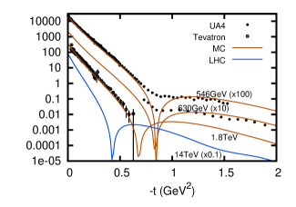
Figure 9: The differential cross section for $pp$ elastic scattering, together with data from UA4 [18] and CDF [19]. The figure also includes a prediction for the LHC.

Fig. 9 shows the elastic $pp$ cross section. As the real part of the amplitude is neglected the diffractive dip is a real zero. The position of this dip can be tuned at one energy, but the change to smaller $t$ at higher energies is a result of the evolution, which cannot be tuned.

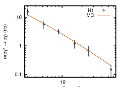
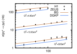
Figure 10: Left: The cross section for $\gamma^{*}p\rightarrow\gamma p$ for $W$ = 82 GeV as function of $Q^{2}$, compared to data from H1 [20]. Right: The cross section for $\gamma^{*}p\rightarrow\rho p$ for $Q^{2}$ = 4.8, 13.5, and 32 $\mathrm{GeV}^{2}$ as function of $W$, compared to data from H1 [21] and ZEUS [22]. Two different wavefunctions have been used for the $\rho$-meson, boosted Gaussian (solid line) and DGKP (dashed line).

Quasielastic $\gamma^{*}p$ scattering is also well reproduced by the model, including the dependence on $Q^{2}$, $W$, and $t$. As two examples fig. 10 shows the $Q^{2}$-dependence for DVCS and the $W$-dependence for $\gamma^{*}p\rightarrow\rho p$. For the latter case two different $\rho$-meson wavefunctions were used, a boosted Gaussian wavefunction [23] and the DGKP [24] wavefunction. Both models show similar growth with $W$, but our normalization agrees better with the boosted Gaussian wavefunction.

5.3 Diffraction

As discussed above diffractive excitation is directly determined by the fluctuations in the evolution. As an example, if we calculate the expression

$$\int d^{2}b\{\langle\langle 1-e^{-\sum f_{ij}}\rangle_{L}^{2}\rangle_{R}-\langle 1-e^{-\sum f_{ij}}\rangle_{LR}^{2}\}$$ (9)

in a frame where the right-moving proton is evolved $y_{R}$ rapidity units, it gives the cross section for single diffractive excitation of this proton to masses satisfying $M_{X}^{2}<M_{0}^{2}\exp(y_{R})$, with $M_{0}\sim 1$ GeV. Here $L$ and $R$ indicate averages over left- and right-moving proton cascades respectively. The result obtained when varying $y_{R}$ is shown in fig. 11a compared with corresponding results from the Tevatron.

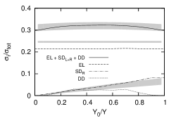
Figure 11: Left: The ratio between the total diffractive and the total cross sections (solid line) together with the contribution from elastic (dashed), single-right (dash-dotted), and double diffractive (dotted) cross sections at 1.8 TeV. The shaded bands are estimates from CDF data [25]. Right: The impact parameter profile for dipole-proton collisions for a initial dipole size $r=2\,\mathrm{GeV}^{-1}\approx 0.4\,$fm at two different energies, $Y=\ln s=$ 9 and 11. Our results (solid and dashed lines) are compared to those from the Kowalski-Teaney [26] model (dot-dashed and dotted lines)

We also note that as the fluctuations in the evolution are quite large, less fluctuations are needed in the impact parameter profile. Thus this profile is more gray, and less black and white, than in fits where the fluctuations in the evolution are not taken into account. This is seen in fig. 11b, which shows a comparison between our model and the result by Kowalski and Teaney [26] for the scattering of a dipole against a proton. In the latter analysis the fluctuations in the evolution are not included.

6 Summary

• A new dipole formulation of high energy collisions in transverse coordinate space is presented

• It has the following main ingredients:

  • NLL corrections to BFKL

  • Non-linear effects: saturation and multiple subcollisions

  • Confinement effects

  • Includes momentum-impact parameter correlations

  • Simple proton and photon models

  • MC implementation

• It gives a fair description of data for:

  • Total cross sections for $pp$ and $\gamma^{*}p$ collisions

  • (Quasi-)elastic scattering in $pp$ and $\gamma^{*}p$

  • Diffractive excitation

• To come soon: Generation of exclusive final states

• Wanted: Better understanding of the connection to the $t$-channel picture of pomeron loops

References

- [1] E. Avsar, G. Gustafson, and L. Lönnblad, JHEP 0507 (2005) 062, ibid 0701 (2007) 012, ibid 0712 (2005) 012.
- [2] C. Flensburg, G. Gustafson, and L. Lönnblad, arXiv:0807.0325, in press in EPJC.
- [3] K. Golec-Biernat and M. Wüsthoff, Phys. Rev. D59 (1999) 014017, ibid D60 (1999) 114023.
- [4] J. Bartels, K. Golec-Biernat, and H. Kowalski (DESY), Phys. Rev. D66 (2002) 014001.
-
[5]
T. Sjöstrand and M. van Zijl, Phys. Rev.
D36 (1987) 2019,
T. Sjöstrand and P.Z. Skands, Eur.Phys.J. C39 (2005) 129. - [6] R. Field, see talks available from http://www.phys.ufl.edu/~rfield/cdf.
- [7] T. Sjöstrand, talk at the 2008 CTEQ - MCnet Summer School on QCD Phenomenology and Monte Carlo Event Generators, Debrecen, Hungary, 2008.
- [8] CDF Coll., F. Abe et al., Phys. Rev. D56 (1997) 3811.
-
[9]
D. Cline, F. Halzen, and J. Luthe, Phys. Rev. Lett.
31 (1973) 491,
S.D. Ellis and M.B. Kislinger, Phys. Rev. D9 (1974) 2027,
L. Durand and P. Hong, Phys. Rev. Lett. 58 (1987) 303. -
[10]
G. Gustafson and G. Miu, Phys. Rev. D63 (2001)
034004,
G. Gustafson, L. Lönnblad, and G. Miu, Phys. Rev. D67 (2003) 034020. -
[11]
A.H. Mueller, Nucl. Phys. B415 (1994) 373,
A.H. Mueller and B. Patel, Nucl. Phys. B425 (1994) 471,
A.H. Mueller, Nucl. Phys. B437 (1995) 107. - [12] A.H. Mueller and G.P. Salam, Nucl. Phys. B475 (1996) 293.
- [13] G.P. Salam, Acta Phys. Polon. B30 (1999) 3679.
- [14] E. Avsar and Y. Hatta, JHEP 0809 (2008) 102.
- [15] R. Corke, Proc. 1st Int. Workshop on Multiple Partonic Interactions at the LHC (MPI@LHC), Perugia, Italy, Oct. 2008, arXiv:0901.2852 [hep-ph].
- [16] H1 Coll., C. Adloff et al., Eur. Phys. J. C21 (2001) 33.
- [17] ZEUS Coll., J. Breitweg et al., Phys. Lett. B487 (2000) 53.
- [18] UA4 Coll., D. Bernard et al., Phys. Lett. B171 (1986) 142.
- [19] CDF Coll., F. Abe et al., Phys. Rev. D50 (1994) 5518.
- [20] H1 Coll., A. Aktas et al., Eur. Phys. J. C44 (2005) 1.
- [21] H1 Coll., C. Adloff et al., Eur. Phys. J. C13 (2000) 371.
- [22] ZEUS Coll., J. Breitweg et al., Eur. Phys. J. C6 (1999) 603.
- [23] J.R. Forshaw, R. Sandapen, and G. Shaw, Phys. Rev. D69 (2004) 094013.
- [24] H.G. Dosch, T. Gousset, G.Kulzinger, and H.J.Pirner, Phys. Rev. D55 (1997) 2602.
- [25] CDF Coll., F. Abe et al., Phys. Rev. D50 (1994) 5535, 5550.
- [26] H. Kowalski and D. Teaney, Phys. Rev. D68 (2003) 114005.