Spectral Curves and Localization
in Random Non-Hermitian Tridiagonal Matrices

Abstract

Eigenvalues and eigenvectors of non-Hermitian tridiagonal periodic random matrices are studied by means of the Hatano-Nelson deformation. The deformed spectrum is annular-shaped, with inner radius measured by the complex Thouless formula. The inner bounding circle and the annular halo are stuctures that correspond to the two-arc and wings observed by Hatano and Nelson in deformed Hermitian models, and are explained in terms of localization of eigenstates via a spectral duality and the Argument principle.

I Introduction

Hermitian tridiagonal random matrices are studied in great detail, and many results are available on spectral properties such as density, statistics and localization of eigenvectors. They appear in several models of physics, as Dyson’s random chains, Anderson’s models for transport in disordered potentials, Ising spin models with random couplings, $\beta$-ensembles of tridiagonal random matrices. Hatano and NelsonHatano96 introduced a beautiful method to study the localization of eigenvectors, by forcing an asymmetry of upper and lower nondiagonal elements. Then the eigenvalues are driven from the real axis to curves in the complex plane, in patterns that measure the localization length of the corresponding eigenvectors.

Tridiagonal random matrices that are non-Hermitian from the start are less studied. They model systems with asymmetric hopping amplitudesDerrida00 ; Goldsheid00 ; Zee03 , describe properties of 1D random walksCicuta00 ; Bauer02 or the evolution of population biologyShnerb98 . Their spectrum is complex. In this work we study how the Hatano-Nelson deformation modifies it, the occurrence of spectral curves and the connection with the localization of eigenvectors.

Let us then consider complex tridiagonal matrices with corners

$$M=\left[\begin{array}[]{cccc}a_{1}&b_{1}&{}\hfil&c_{1}\\ c_{2}&\ddots&\ddots&{}\hfil\\ {}\hfil&\ddots&\ddots&b_{n-1}\\ b_{n}&{}\hfil&c_{n}&a_{n}\\ \end{array}\right]$$ (5)

where all matrix elements are i.i.d. complex random variables. Here we use the uniform distribution in the unitary disk of the complex plane. This implies that the eigenvalue density of the ensemble is only a function of the modulus of the eigenvalue. The eigenvalues of a sample matrix of size $n=800$ are shown in Fig.1 (left).

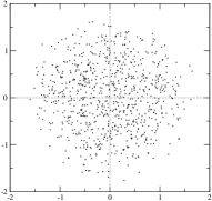
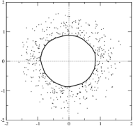
Figure 1: Eigenvalues in the complex plane of a single non Hermitian tridiagonal matrix of size $n=800$. The same matrix entries $\{a_{k},b_{k},c_{k}\}$ are used, with $\xi=0$ and $\varphi=0$ (left), and $\xi=0.5$ and $\varphi=0$ (right). Note that the eigenvalues out of the circle have the same positions in the both cases.

We next consider two deformations of the matrix $M$, by a complex parameter $z=e^{\xi+i\varphi}$:

$$M(z^{n})=\left[\begin{array}[]{cccc}a_{1}&b_{1}&{}\hfil&z^{n}c_{1}\\ c_{2}&\ddots&\ddots&{}\hfil\\ {}\hfil&\ddots&\ddots&b_{n-1}\\ b_{n}/z^{n}&{}\hfil&c_{n}&a_{n}\\ \end{array}\right],$$ (10)

$$M_{b}(z)=\left[\begin{array}[]{cccc}a_{1}&b_{1}/z&{}\hfil&zc_{1}\\ zc_{2}&\ddots&\ddots&{}\hfil\\ {}\hfil&\ddots&\ddots&b_{n-1}/z\\ b_{n}/z&{}\hfil&zc_{n}&a_{n}\\ \end{array}\right].$$ (15)

The two matrices are similar, $M_{b}(z)=SM(z^{n})S^{-1}$, through a diagonal matrix with entries $S_{ii}=z^{i}$. The balanced matrix $M_{b}(z)$ is more convenient for numerical work. Since the matrices share the same set of eigenvalues, a rotation of $z$ by $2\pi/n$ does not change the eigenvalues of $M_{b}(z)$.

The eigenvalues of $M_{b}(z)$ are shown in Fig.1 (right). The distribution looks remarkable: a “circle” centered in the origin bounds an outer annular halo where the eigenvalues appear exactly in the same positions as those in the left figure. The inner region is void: all the eigenvalues that were there before deformation ($\xi=0$) have moved to the boundary circle.

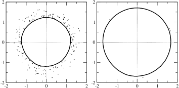
Figure 2: The same random matrix entries as in Fig.1 with $\xi=0.7$ and $\varphi=0$ (left), $\xi=1$ and $\varphi=0$ (right).

As $|z|$ becomes larger, see Fig.2, the circle enlarges as well, but the eigenvalues in the annular halo do not move, until they are swept by the circle. For large $\xi$ only the circle remains. This is not surprising: in the limit of large $|z|$ the matrix $M_{b}(z)$ simplifies to bidiagonal. The eigenvalue equation can be solved explicitly and gives $E^{n}=z^{n}b_{1}\cdots b_{n}$. Then the eigenvalues $E_{k}=|z|e^{\langle\ln|b|\rangle}\exp i(\theta+2\pi k/n)$ are equally spaced and lie on a circle of radius $r$ such that $\log r=\xi+\langle\log|b|\rangle$.

Eigenvalues on the circle and in the halo respond differently to the phase $\varphi={\rm arg}\,z$. As $\varphi$ sweeps the Brillouin zone from 0 to $2\pi/n$, only the eigenvalues sitting on the circle move (and remain therein), while the outer ones do not have measurable changes at all. This is illustrated in Fig.3, which also shows that an eigenvalue on the circle moves to the position of a neighboring one as $\varphi$ is increased by $2\pi/n$.

Figure 3: Motion in the complex plane of the eigenvalues of a single non Hermitian tridiagonal matrix of size $n=100$ as the phase $\varphi$ is changed in half of its range. The same matrix entries are used, with $\xi=0.5$ (left) and $\xi=1$ (right). Eigenvalues not belonging to the loop are seen to be fixed, corresponding to localized states. The loop becomes closed if the whole angular range is evaluated.

Figure 4: Eigenvalues in the complex plane of 3 different samples of size $n=400$ (left) and $n=1200$ (right). All matrices with $\xi=0.5$ and $\varphi=0$.

By increasing the size $n$ of the matrices, the “circle” is seen to become independent of the sample and more regular, (Fig.4).

Figure 5: Eigenvalues of a single Hatano-Nelson tridiagonal matrix of size $n=600$, with $\xi=1$, $b_{k}=c_{k}=1$ and random numbers $a_{k}$ uniformly distributed in $(-3.5,3.5)$. They belong to two arcs or two wings in the real axis, which are the residuate of the undeformed spectrum.

The phenomenon described is analogous to what Hatano and NelsonHatano96 discovered for random tridiagonal Hermitian matrices ($a_{k}$ real, $c_{k+1}=b_{k}^{*}$) where the undeformed eigenvalues ($\xi=0$) are real. The deformation forces them to move into the complex plane and distribute along a two-arc loop, with possible external wings of unaffected eigenvalues in the real axis (Fig.5). The two-arc loop and wings of the Hermitian model correspond to the circle and annular halo of the non-Hermitian model discussed here.

In Section II and III we study the spectral density of the undeformed ensemble and the localization of eigenvectors, measured by the Lyapunov exponent or by the variance. In Section IV we explain the observed spectral features of the deformed ensemble by means of the Argument Principle of complex analysis and a spectral duality between the eigenvalues of $M(z^{n})$ and those of the transfer matrix.

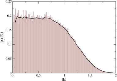
Figure 6: Eigenvalue density $\rho_{0}(|E|)$ of the undeformed ensemble (matrix size $n=1000$, 100 samples). The dark line is obtained by smoothing the hystogram data on local windows of 10 bins (out of 300). The plateau is fitted by the value $0.193(2)$.

II The spectrum of $M$

Since the matrix entries of $M$ are chosen to be uniformly distributed in the unit complex disk, the average eigenvalue density of the ensemble, $\rho_{0}(E)=\langle\frac{1}{n}\sum_{i}\delta_{2}(E-E_{i})\rangle$, depends on $|E|$. The eigenvalue equation

$$c_{k}\,u_{k-1}+a_{k}\,u_{k}+b_{k}\,u_{k+1}=E\,u_{k}$$ (16)

written for the component $u_{k}$ with highest absolute value, implies the inequality $|E|\leq|a_{k}|+|b_{k}|+|c_{k}|\leq 3$. Thus the disk that supports the density has a radius not exceeding $3$; the numerical evidence is that it has length $2$.

We diagonalized 100 matrices of size $n=1000$ to obtain numerically the density of eigenvalues $\rho_{0}(|E|)$ shown in Fig.6. The lowest moments $\mu_{k}=\langle\frac{1}{n}\sum_{i}|E_{i}|^{k}\rangle$= $2\pi\int_{0}^{2}dxx^{k+1}\rho_{0}(x)$ are also evaluated: $\mu_{1}=0.9107(12)$, $\mu_{2}=0.9678(22)$, $\mu_{3}=1.1327(36)$ and $\mu_{4}=1.4204(59)$.

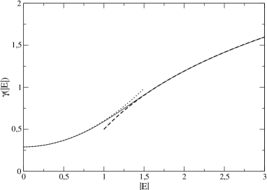
Figure 7: The Lyapunov exponent $\gamma(|E|)$ evaluated numerically (100 matrices of size $n=1000$). The two curves are a quadratic fit near the origin, $0.2914(1)+0.309(0)|E|^{2}$, and the exact analytic expression $\lg(|E|)+1/2$ of $\gamma$ for $|E|>2$. The fit near the origin is consistent with the value found for $\rho_{0}(0)$ (via Poisson equation).

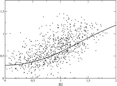
Figure 8: Pairs $(|E_{a}|,\gamma_{a})$, where $E_{a}$ are eigenvalues and $\gamma_{a}$ are rates of exponential localization, for the eigenvectors of a matrix $M$ of size $n=800$ ($\xi=0$). The continuous line is the Lyapunov exponent $\gamma(|E|)$.

III The Lyapunov exponent

The numerical evaluation of the eigenvectors of $M$ shows that they are strongly localized for all eigenvalues; indeed, for large matrix size, they decay exponentially (Anderson localization). The rate of decay is measured by the Lyapunov exponent, an asymptotic property of transfer matrices.

The transfer matrix of a realization $M$ is the product of $2\times 2$ random matrices:

$$t(E)=\prod_{k=1}^{n}\left[\begin{array}[]{cc}b_{k}^{-1}(E-a_{k})&-b_{k}^{-1}c_{k}\\ 1&0\\ \end{array}\right].$$ (19)

Its eigenvalues can be written as $z_{\pm}^{n}=e^{n(\xi_{\pm}+i\varphi_{\pm})}$. For large $n$ the exponents $\xi_{\pm}(E)$ become opposite: $\xi_{+}+\xi_{-}$ $=\frac{1}{n}\log|\det t(E)|$ $=\frac{1}{n}\sum_{k=1}^{n}\log|c_{k}|-\log|b_{k}|\to 0$.

According to the theory of random matrix products, for large $n$ the positive exponent $\xi_{+}$ becomes independent of $n$ and the realization of randomness, and converges to the Lyapunov exponent of the matrix ensemble. The Lyapunov exponent can be evaluated by an extension of Thouless formula to non-Hermitian matricesDerrida00 ; Goldsheid05 ,

$$\gamma(E)=\int d^{2}E^{\prime}\rho_{0}(E^{\prime})\log|E-E^{\prime}|-\langle\log|b|\rangle,$$ (20)

where $\rho_{0}$ is the eigenvalue density of the ensemble of matrices $M$. Note that for complex spectra, the equation for $\gamma$ implies the Poisson equation $\nabla^{2}\gamma(E)=2\pi\rho_{0}(E)$. Therefore $\gamma(E)$ can be understood as the electrostatic potential generated by a charge distribution in the plane with density $\rho_{0}(E)$.

For a distribution of matrix entries that is uniform in the unit disk, it is $\langle\log|b|\rangle=-1/2$ and $\rho_{0}$ is rotation invariant. Then the integral can be simplified:

$$\gamma(|E|)= \log|E|\,{\cal N}_{0}(|E|)$$ (21)

$$+2\pi\int_{|E|}^{\infty}dE^{\prime}E^{\prime}\rho_{0}(E^{\prime})\log E^{\prime}+1/2.$$

The integral $\int_{0}^{2\pi}\log|r-r^{\prime}e^{i\varphi}|d\varphi=2\pi\log{\rm max}(r,r^{\prime})$ was used. ${\cal N}_{0}(|E|)$ is the fraction of the spectrum inside the disk of radius $|E|$. For $|E|$ larger than the spectral radius it is

$$\gamma(|E|)=\log(|E|)+1/2,\quad|E|\geq 2.$$ (22)

The Lyapunov exponent is an increasing function of $|E|$. Its numerical evaluation is shown in Fig.7.

We checked numerically the exponential decay of eigenvectors with a rate given by $\gamma(|E|)$. If $\vec{u}$ is an eigenvector of $M$, with components $\{u_{k}\}_{k=1}^{n}$, the numbers $|u_{k}|^{2}$ provide the probability distribution for the position of a particle in the lattice $1\ldots n$. We choose to measure the localization of the eigenvector by the variance in position:

$${\rm var}[\vec{u}]=\left(\sum_{k=1}^{n}|u_{k}|^{2}(k-\overline{k})^{2}\right)^{1/2},$$ (23)

where $\overline{k}=\sum_{k}k|u_{k}|^{2}$ is the mean position of the particle. Other measures could be used, as the inverse participation ratio or the Shannon entropy; in this case the eigenvectors are peaked on small intervals, and the variance has a clear meaning.

For an ideal state $\vec{v}$ that is exponentially localized, $|v_{k}|^{2}=(\tanh\gamma)\,e^{-2\gamma|k|}$, ($\gamma n\gg 1$), the variance is ${\rm var}[\vec{v}]=\sinh(1/\gamma)$. We use the same relation to compute a rate $\gamma_{a}$ from the numerically evaluated variance of an eigenstate $\vec{u}_{a}$. In Fig.8 we plot the numerical pairs $(|E_{a}|,\gamma_{a})$ for the eigenvalues and eigenvectors of a single matrix $M$ of size $n=800$, together with the Lyapunov exponent $\gamma(|E|)$, given by Thouless formula (21). The numerical data are consistent with the picture of exponential localization of eigenvectors.

Figure 9: Variance of eigenvectors ($z$-axis) and corresponding eigenvalues ($x=ReE$, $y=ImE$) of a random matrix $M_{b}(e^{\xi})$ of size $n=800$ and $\xi=\log 2$. The radius of the hole is approximately 1.16.

IV Hole, halo and localization

When the parameter $\xi$ is switched on, it appears in the corners of the matrix $M(z^{n})$ and modifies the boundary conditions in (16). In the transition from $M$ to $M(z^{n})$, one expects that the eigenvalues of enough localized eigenstates do not change. An eigenstate $\vec{u}=\{u_{k}\}$ of $M(z^{n})$ corresponds to an eigenstate $S\vec{u}$ of $M_{b}(z)$, with components $z^{k}u_{k}$. If $|u_{k}|\approx e^{-\gamma|k|}$ for large $k$, the factor $e^{k\xi}$ delocalizes it if $\gamma<\xi$. This simple argument by Hatano and Nelson indicates a threshold value $\gamma(|E|)=\xi$ at which eigenvalues must be drastically influenced by the deformation.

In Fig.9 we plot the variances ($z$ axis) of the eigenvectors of a matrix $M_{b}(z=2)$ of size $n=800$, and the corresponding complex eigenvalues (horizontal plane). The boundary of the circular hole is populated by the eigenvectors which are delocalized.

The existence of an empty disk and a halo of fixed eigenvalues for the deformed ensemble thus reflects the localization properties of the eigenvectors of $M$ as a function of $|E|$, i.e. the function $\gamma(|E|)$.

Proposition: in the large $n$ limit, $M_{b}(e^{\xi+i\varphi})$ has no eigenvalues in the disk of radius $r$, where

$$\gamma(r)=\xi$$ (24)

Proof: The hole in the spectrum of $M_{b}(z)$ can be understood via the Argument Principle of complex analysis: the number of zeros of the analytic function $f(E)=\det[E-M_{b}(z)]$ inside a disk of radius $r$ is equal to the variation of arg$f(E)/2\pi$ along the contour of the disk.

The function $f(E)$ is related to the eigenvalues $z^{n}_{\pm}(E)$ of the transfer matrix $t(E)$ by a duality identityMolinari08 ; Molinari :

$$\det[E-M_{b}(z)]=-\frac{1}{z^{n}}(b_{1}\cdots b_{n})\det[t(E)-z^{n}]$$ (25)

Then

$${\rm arg}\det[E-M_{b}(e^{\xi+i\varphi})]={\rm const.}$$

$$+{\rm arg}[e^{n(\xi_{+}-\xi)+in(\varphi_{+}-\varphi)}-1]$$

$$+{\rm arg}[e^{n(\xi_{-}-\xi)+i(\varphi_{-}-\varphi)}-1]$$

Let us fix $\xi>0$ and take the large $n$ limit. Then: $\xi_{+}>0$ and $\xi_{-}<0$; ${\rm arg}[e^{n(\xi_{+}-\xi)+in(\varphi_{+}-\varphi)}-1]$ equals $n(\varphi_{+}-\varphi)$ if $\xi_{+}>\xi$, and $\pi$ if $\xi>\xi_{+}$; ${\rm arg}[e^{n(\xi_{-}-\xi)+in(\varphi_{-}\varphi)}-1]=\pi$ always. We also identify $\xi_{+}(E)$ with the Lyapunov exponent $\gamma(|E|)$. The variation of arg$f(E)/2\pi$ along a circumference of radius $r$ is zero if $\xi>\gamma(r)$. $\Box$

Since $\gamma(0)$ is nonzero, there is a threshold value $\xi_{min}\approx 0.291$ below which no hole opens in the spectral support.

V Conclusions

The Hatano Nelson deformation opens a hole in the spectrum of non Hermitian tridiagonal random matrices with i.i.d. matrix elements. The eigenvalues that are swept to the boundary of the hole correspond to states that are no longer Anderson localized. This is explained in terms of a spectral duality, stability of the Lyapunov exponent, and the Argument Principle.

Tridiagonal matrices with different strengths of randomness in the three diagonals would also show similar spectral features.

Aknowledgements: L.G.M. wishes to thank prof. I. Goldsheid for having inspired him the present investigation, and for useful comments.

References

- (1) N. Hatano and D. R. Nelson, Localization transition in non-Hermitian quantum mechanics, Phys. Rev. Lett. 77 (1996) 570–3.
- (2) B. Derrida, J. L. Jacobsen and R. Zeitak, Lyapunov exponent and density of states of a one-dimensional non-Hermitian Schrödinger equation, J. Stat. Phys. 98 (2000) 31–55.
- (3) I. Ya. Goldsheid and B. Khoruzhenko, Eigenvalue curves of asymmetric tridiagonal random matrices, Electronic Journal of Probability 5 (2000) 1–28.
- (4) D. E. Holz, H. Orland and A. Zee, On the remarkable spectrum of a non-Hermitian random matrix model, J. Phys. A: Math. Gen. 36 (2003) 3385–3400.
- (5) G. M. Cicuta, M. Contedini and L. Molinari, Non-Hermitian tridiagonal random matrices and returns to the origin of a random walk, J. Stat. Phys. 98 (2000) 685–99.
- (6) M. Bauer, D. Bernard and J. M. Luck, Even-visiting random walks: exact and asymptotic results in one dimension, J. Phys. A: Math. Gen. 34 (2002) 2659–79.
- (7) D. R. Nelson and N. M. Shnerb, Non-Hermitian localization and population biology, Phys. Rev. E 58 (1998) 1383-1403.
- (8) I. Ya. Goldsheid and B. Khoruzhenko, Thouless formula for random non-Hermitian Jacobi matrices, Isr. J. of Math. 148 (2005) 331–46.
- (9) L. G. Molinari, Determinants of block-tridiagonal matrices, Linear Algebra and its Applications 429 (2008) 2221–6.
- (10) L. G. Molinari, Non Hermitian spectra and Anderson Localization, arXiv:0808.1241 [math-ph], to appear on J. Phys. A: Math. Theor.