KEK-CP-223

Pion form factors from two-flavor lattice QCD with exact chiral symmetry

S. Aokia,b, T. W. Chiuc, H. Fukayad, S. Hashimotoe,f, T. H. Hsiehg, T. Kanekoe,f, H. Matsufuruh, J. Noakie, T. Onogii, E. Shintanii and N. Yamadae,f
(JLQCD and TWQCD collaborations)
aGraduate School of Pure and Applied Sciences, University of Tsukuba, Ibaraki 305-8571, Japan
bRiken BNL Research Center, Brookhaven National Laboratory, Upton, New York 11973, USA
cPhysics Department, Center for Theoretical Sciences, and Center for Quantum Science and Engineering, National Taiwan University, Taipei, 10617, Taiwan
dDepartment of Physics, Nagoya University, Nagoya 464-8602, Japan
eKEK Theory Center, High Energy Accelerator Research Organization (KEK), Ibaraki 305-0801, Japan
fSchool of High Energy Accelerator Science, The Graduate University for Advanced Studies (Sokendai), Ibaraki 305-0801, Japan
gResearch Center for Applied Sciences, Academia Sinica, Taipei 115, Taiwan
hComputing Research Center, High Energy Accelerator Research Organization (KEK), Ibaraki 305-0801, Japan
iYukawa Institute for Theoretical Physics, Kyoto University, Kyoto 606-8502, Japan
Abstract

We calculate pion vector and scalar form factors in two-flavor lattice QCD and study the chiral behavior of the vector and scalar radii r2V,Ssubscriptdelimited-⟨⟩superscript𝑟2𝑉𝑆\langle r^{2}\rangle_{V,S}. Numerical simulations are carried out on a 163×32superscript1633216^{3}\times 32 lattice at a lattice spacing of 0.12 fm with quark masses down to ms/6similar-toabsentsubscript𝑚𝑠6\sim\!m_{s}/6, where mssubscript𝑚𝑠m_{s} is the physical strange quark mass. Chiral symmetry, which is essential for a direct comparison with chiral perturbation theory (ChPT), is exactly preserved in our calculation at finite lattice spacing by employing the overlap quark action. We utilize the so-called all-to-all quark propagator in order to calculate the scalar form factor including the contributions of disconnected diagrams and to improve statistical accuracy of the form factors. A detailed comparison with ChPT reveals that the next-to-next-to-leading-order contributions to the radii are essential to describe their chiral behavior in the region of quark mass from ms/6subscript𝑚𝑠6m_{s}/6 to ms/2subscript𝑚𝑠2m_{s}/2. Chiral extrapolation based on two-loop ChPT yields r2V=0.409(23)(37)fm2subscriptdelimited-⟨⟩superscript𝑟2𝑉0.4092337superscriptfm2\langle r^{2}\rangle_{V}\!=\!0.409(23)(37)~{}\mbox{fm}^{2} and r2S=0.617(79)(66)fm2subscriptdelimited-⟨⟩superscript𝑟2𝑆0.6177966superscriptfm2\langle r^{2}\rangle_{S}\!=\!0.617(79)(66)~{}\mbox{fm}^{2}, which are consistent with phenomenological analysis. We also present our estimates of relevant low-energy constants.

I Introduction

Recent algorithmic improvements allow us to perform large-scale simulations of unquenched QCD in the chiral regime with various lattice discretizations. Calculation of phenomenologically important quantities has then become feasible. In order to make reliable prediction for physical observables, it is crucial to examine the consistency of their chiral behavior with expectations from chiral perturbation theory (ChPT). Lattice QCD with exact chiral symmetry is the cleanest framework for this purpose, while conventional lattice actions may distort chiral behavior of observables by their explicit symmetry breaking, especially when one goes beyond the next-to-leading order (NLO) in ChPT. The JLQCD and TWQCD collaborations embarked on the simulations with exact chiral symmetry Lat07:JLQCD:Matsufuru ; Lat08:JLQCD:Hashimoto employing the overlap quark action Overlap:NN ; Overlap:N . So far, we have performed a detailed study of the pion mass and decay constant in two-flavor lattice QCD Spectrum:Nf2:RG+Ovr:JLQCD . For other physics results from this project, see e-regime:eigen:Nf2:RG+Ovr:JLQCD:1 ; chi_t:Nf2:RG+Ovr:JLQCD+TWQCD ; e-regime:msn:Nf2:RG+Ovr:JLQCD ; e-regime:eigen:Nf2:RG+Ovr:JLQCD:2 ; B_K:Nf2:RG+Ovr:JLQCD ; S:Nf2:RG+Ovr:JLQCD ; Sigma:Nf2:RG+Ovr:JLQCD ; OPE:Nf2:RG+Ovr:JLQCD .

The pion vector form factor FV(q2)subscript𝐹𝑉superscript𝑞2F_{V}(q^{2}) defined by

π(p)|Vμ|π(p)quantum-operator-product𝜋superscript𝑝subscript𝑉𝜇𝜋𝑝\displaystyle\langle\pi(p^{\prime})|V_{\mu}|\pi(p)\rangle =\displaystyle= (p+p)μFV(q2),q2=(pp)2,subscript𝑝superscript𝑝𝜇subscript𝐹𝑉superscript𝑞2superscript𝑞2superscript𝑝superscript𝑝2\displaystyle\left(p+p^{\prime}\right)_{\mu}F_{V}(q^{2}),\hskip 14.22636ptq^{2}=(p-p^{\prime})^{2}, (1)

provides a simple testing ground for the consistency between lattice calculation and ChPT. This is one of the fundamental quantities to characterize the low-energy dynamics of pions: for instance, it is related to the charge radius of pion

r2Vsubscriptdelimited-⟨⟩superscript𝑟2𝑉\displaystyle\langle r^{2}\rangle_{V} =\displaystyle= 6FV(q2)q2|q2=0.evaluated-at6subscript𝐹𝑉superscript𝑞2superscript𝑞2superscript𝑞20\displaystyle 6\left.\frac{\partial F_{V}(q^{2})}{\partial q^{2}}\right|_{q^{2}=0}. (2)

The chiral expansion of FV(q2)subscript𝐹𝑉superscript𝑞2F_{V}(q^{2}) and r2Vsubscriptdelimited-⟨⟩superscript𝑟2𝑉\langle r^{2}\rangle_{V} is available up to two loops, namely to the next-to-next-to-leading-order (NNLO), both for Nf=2subscript𝑁𝑓2N_{f}\!=\!2 PFF:ChPT:NLO:1 ; PFF_V:ChPT:NNLO ; PFF_V:ChPT:NNLO:2 and Nf=3subscript𝑁𝑓3N_{f}\!=\!3 PFF:ChPT:NLO:2 ; PFF_V:ChPT:NNLO:Nf3 . Analyses of experimental data based on two-loop ChPT have led to precise estimates of r2Vsubscriptdelimited-⟨⟩superscript𝑟2𝑉\langle r^{2}\rangle_{V} PFF_V:ChPT:NNLO ; PFF_V:ChPT:NNLO:Nf3 , which can also be used as a benchmark of lattice calculations.

From previous lattice studies PFF:Nf2:Plq+Clv:HKL ; PFF:Nf2:DBW2+DW:RBC ; PFF:Nf0:Plq+tmW:AL ; PFF:impG+AT+DWF:LHP ; PFF:Nf2:Plq+Clv:JLQCD ; PFF:Nf2:Plq+Clv:QCDSF ; PFF:Nf0:LW+CImp:BGR ; PFF:Nf3:RG+DW:RBC+UKQCD ; PFF:Nf2:Sym+tmW:ETMC , the consistency with experiment has not been established convincingly: some of them reported good agreement with experiment PFF:Nf2:Plq+Clv:QCDSF ; PFF:Nf3:RG+DW:RBC+UKQCD ; PFF:Nf2:Sym+tmW:ETMC , whereas others underestimated r2Vsubscriptdelimited-⟨⟩superscript𝑟2𝑉\langle r^{2}\rangle_{V} significantly PFF:Nf2:Plq+Clv:HKL ; PFF:impG+AT+DWF:LHP ; PFF:Nf2:Plq+Clv:JLQCD ; PFF:Nf0:LW+CImp:BGR . This is possibly due to systematics in the parametrization of the q2superscript𝑞2q^{2} dependence of FV(q2)subscript𝐹𝑉superscript𝑞2F_{V}(q^{2}) and to the chiral extrapolation of r2Vsubscriptdelimited-⟨⟩superscript𝑟2𝑉\langle r^{2}\rangle_{V}. For instance, the NNLO chiral corrections are fully taken into account in the ChPT analyses but not in most of the previous lattice studies. They could significantly modify the chiral behavior of r2Vsubscriptdelimited-⟨⟩superscript𝑟2𝑉\langle r^{2}\rangle_{V} at up and down quark masses larger than their physical value, as demonstrated in our report Lat08:JLQCD:TK and more recently in Ref. PFF:Nf2:Sym+tmW:ETMC with a different lattice discretization. Our simulations with exact chiral symmetry enable us to perform more stringent test of the chiral behavior of lattice data using two-loop ChPT without suffering from the distortion due to explicit chiral symmetry breaking present in other frameworks.

The chiral behavior of the scalar form factor FS(q2)subscript𝐹𝑆superscript𝑞2F_{S}(q^{2}) defined by

π(p)|S|π(p)quantum-operator-product𝜋superscript𝑝𝑆𝜋𝑝\displaystyle\langle\pi(p^{\prime})|S|\pi(p)\rangle =\displaystyle= FS(q2)subscript𝐹𝑆superscript𝑞2\displaystyle F_{S}(q^{2}) (3)

is another interesting subject, since i) its radius

r2Ssubscriptdelimited-⟨⟩superscript𝑟2𝑆\displaystyle\langle r^{2}\rangle_{S} =\displaystyle= 6FS(q2)q2|q2=0evaluated-at6subscript𝐹𝑆superscript𝑞2superscript𝑞2superscript𝑞20\displaystyle 6\left.\frac{\partial F_{S}(q^{2})}{\partial q^{2}}\right|_{q^{2}=0} (4)

provides a determination of the low energy constant (LEC) l4subscript𝑙4l_{4} alternative to that with the decay constant Fπsubscript𝐹𝜋F_{\pi}, and ii) r2Ssubscriptdelimited-⟨⟩superscript𝑟2𝑆\langle r^{2}\rangle_{S} has 6 times enhanced chiral logarithm compared to r2Vsubscriptdelimited-⟨⟩superscript𝑟2𝑉\langle r^{2}\rangle_{V} and thus may offer an opportunity to clearly identify the one-loop chiral logarithm. Since there are no experimental processes directly related to FS(q2)subscript𝐹𝑆superscript𝑞2F_{S}(q^{2}), its direct determination is possible only through lattice QCD. It is however difficult to evaluate disconnected correlation functions with conventional point-to-all quark propagator, which flows from a fixed lattice site to any site. There have been only a few calculations of FS(q2)subscript𝐹𝑆superscript𝑞2F_{S}(q^{2}) PFF:Nf2:Plq+Clv:JLQCD ; PFF:Nf0:LW+CImp:BGR , and the contributions of disconnected diagrams were ignored in these studies.

In this paper, we calculate the pion vector and scalar form factors FV,S(q2)subscript𝐹𝑉𝑆superscript𝑞2F_{V,S}(q^{2}) in two-flavor QCD and study the chiral behavior of the radii r2V,Ssubscriptdelimited-⟨⟩superscript𝑟2𝑉𝑆\langle r^{2}\rangle_{V,S}. For a detailed comparison with two-loop ChPT, we preserve chiral symmetry by employing the overlap quark action and simulate up and down quarks with masses as low as mms/6similar-to𝑚subscript𝑚𝑠6m\!\sim\!m_{s}/6. The scalar form factor FS(q2)subscript𝐹𝑆superscript𝑞2F_{S}(q^{2}) is evaluated including the contribution of disconnected diagrams by using the all-to-all quark propagator, which contains propagations from any lattice site to any site. The all-to-all propagator is also helpful to substantially improve statistical accuracy of FV,S(q2)subscript𝐹𝑉𝑆superscript𝑞2F_{V,S}(q^{2}). Our preliminary analyses based on one- and two-loop ChPT have been reported in Refs. Lat07:JLQCD:TK and Lat08:JLQCD:TK , respectively.

This paper is organized as follows. We introduce our simulation method in Sec. II. Calculation of the form factors from pion correlators is presented in Sec III. We parametrize their q2superscript𝑞2q^{2} dependence in Sec. IV. Section V is devoted to a detailed description of our chiral extrapolation of the radii. Finally, our concluding remarks are given in Sec. VI.

II Simulation method

II.1 Configuration generation

We calculate pion form factors in QCD with dynamical up and down quarks with a degenerate mass parameter. Numerical simulations are carried out with the Iwasaki gauge action Iwasaki and the overlap quark action Overlap:NN ; Overlap:N , which has exact chiral symmetry at finite lattice spacings lat_chial_sym . Its Dirac operator is given by

D(m)𝐷𝑚\displaystyle D(m) =\displaystyle= (m0+m2)+(m0m2)γ5sgn[HW(m0)],subscript𝑚0𝑚2subscript𝑚0𝑚2subscript𝛾5sgndelimited-[]subscript𝐻Wsubscript𝑚0\displaystyle\left(m_{0}+\frac{m}{2}\right)+\left(m_{0}-\frac{m}{2}\right)\gamma_{5}\,{\rm sgn}\left[H_{\rm W}(-m_{0})\right], (5)

where m𝑚m is the quark mass and HW(m0)=γ5DW(m0)subscript𝐻Wsubscript𝑚0subscript𝛾5subscript𝐷Wsubscript𝑚0H_{\rm W}(-m_{0})\!=\!\gamma_{5}D_{\rm W}(-m_{0}) is the Hermitian Wilson-Dirac operator. We set the mass parameter of this kernel operator to m0=1.6subscript𝑚01.6-m_{0}\!=\!-1.6, with which the locality of the overlap Dirac operator is confirmed Lat06:JLQCD:Yamada ; Prod_Run:JLQCD:Nf2:RG+Ovr . Because of the sign function sgn[HW(m0)]sgndelimited-[]subscript𝐻Wsubscript𝑚0{\rm sgn}[H_{\rm W}(-m_{0})] in D(m)𝐷𝑚D(m), the overlap action is discontinuous when HW(m0)subscript𝐻Wsubscript𝑚0H_{\rm W}(-m_{0}) develops zero eigenvalue(s). The commonly-used Hybrid Monte Carlo (HMC) algorithm can be modified to deal with this discontinuity overlap:HMC:FKS but turned out to be very costly. In order to carry out high-statistics simulations, we suppress (near-)zero modes of HW(m0)subscript𝐻Wsubscript𝑚0H_{\rm W}(-m_{0}) by introducing an auxiliary determinant

ΔWsubscriptΔW\displaystyle\Delta_{\rm W} =\displaystyle= det[HW(m0)2]det[HW(m0)2+μ2]delimited-[]subscript𝐻Wsuperscriptsubscript𝑚02delimited-[]subscript𝐻Wsuperscriptsubscript𝑚02superscript𝜇2\displaystyle\frac{\det[H_{\rm W}(-m_{0})^{2}]}{\det[H_{\rm W}(-m_{0})^{2}+\mu^{2}]} (6)

into the Boltzmann weight exW:Vranas ; exW+extmW:JLQCD . We note that this can be considered as an O(a2)𝑂superscript𝑎2O(a^{2}) modification of the gauge action, and hence does not change the continuum limit of the theory. The parameter μ𝜇\mu is tuned to 0.2 so as to minimize lattice artifacts induced by ΔWsubscriptΔW\Delta_{\rm W} Lat06:JLQCD:Yamada ; exW+extmW:JLQCD . We refer readers to Ref. Prod_Run:JLQCD:Nf2:RG+Ovr for further details of our simulation method.

An important property of the determinant ΔWsubscriptΔW\Delta_{\rm W} is that it fixes the global topological charge Q𝑄Q of the gauge field during continuous updating of the gauge configuration in the HMC algorithm. Note, however, that local topological fluctuations are present, and the topological susceptibility calculated in Ref. chi_t:Nf2:RG+Ovr:JLQCD+TWQCD shows expected behavior as a function of sea quark mass. As shown in Refs. fixed_Q:BCNW ; fixed_Q:AFHO , the effect of fixed global topology can be considered as a finite volume effect and is suppressed by the inverse of the space-time volume V𝑉V. Furthermore the effect can be systematically corrected by investigating Q𝑄Q dependence of physical observables of interest  fixed_Q:AFHO .

Our gauge ensembles are generated on a 163×32superscript1633216^{3}\times 32 lattice. The bare gauge coupling is β=6/g2=2.30𝛽6superscript𝑔22.30\beta\!=6/g^{2}\!=\!2.30 where the lattice spacing determined from the Sommer scale r0=0.49subscript𝑟00.49r_{0}\!=\!0.49 fm r0 is a=0.1184(21)𝑎0.118421a\!=\!0.1184(21) fm. In the trivial topological sector Q=0𝑄0Q\!=\!0, we take four values of bare up and down quark masses, m=0.015𝑚0.015m\!=\!0.015, 0.025, 0.035 and 0.050, which cover a range [ms/6,ms/2]subscript𝑚𝑠6subscript𝑚𝑠2[m_{s}/6,m_{s}/2]. At each m𝑚m, we calculate pion form factors using 100 independent configurations separated by 100 HMC trajectories. In order to study the effect of fixed topology, we also simulate non-trivial topological sectors Q=2𝑄2Q\!=\!-2 and 44-4 at m=0.050𝑚0.050m\!=\!0.050 with statistics of 50 independent configurations.

II.2 Construction of all-to-all quark propagator

The conventional method to calculate hadron correlators employs the so-called point-to-all quark propagator which flows from a fixed lattice site to any site. This is however not suitable to calculate disconnected diagrams which involve quark loops starting from and ending at arbitrary lattice sites. In this work, therefore, we construct all-to-all quark propagator that contains the quark propagating from any lattice site to any site along the strategy proposed in Ref. A2A .

Let us consider a decomposition of the quark propagator using eigenmodes of the overlap operator

D1(x,y)superscript𝐷1𝑥𝑦\displaystyle D^{-1}(x,y) =\displaystyle= k1λ(k)u(k)(x)u(k)(y),subscript𝑘1superscript𝜆𝑘superscript𝑢𝑘𝑥superscript𝑢𝑘𝑦\displaystyle\sum_{k}\frac{1}{\lambda^{(k)}}u^{(k)}(x)u^{(k)\dagger}(y), (7)

where λ(k)superscript𝜆𝑘\lambda^{(k)} and u(k)(x)superscript𝑢𝑘𝑥u^{(k)}(x) represent k𝑘k-th lowest eigenvalue and eigenvector of D𝐷D, respectively. Note that the eigenvalues are ordered by their absolute values. Color and spinor indices are suppressed for simplicity. It is expected that low-lying modes dominate low-energy dynamics of pions including their form factors. We evaluate these low-mode contributions to the propagator exactly as

(D1)low(x,y)subscriptsuperscript𝐷1low𝑥𝑦\displaystyle(D^{-1})_{\rm low}(x,y) =\displaystyle= k=1Ne1λ(k)u(k)(x)u(k)(y)(Ne=100)superscriptsubscript𝑘1subscript𝑁𝑒1superscript𝜆𝑘superscript𝑢𝑘𝑥superscript𝑢𝑘𝑦subscript𝑁𝑒100\displaystyle\sum_{k=1}^{N_{e}}\frac{1}{\lambda^{(k)}}\,u^{(k)}(x)u^{(k)\dagger}(y)\hskip 14.22636pt(N_{e}\!=\!100) (8)

using 100 low-lying modes for each gauge configuration. Note that the overlap operator is normal and we do not have to distinguish left and right eigenvectors.

The contribution of higher modes is estimated stochastically by the noise method with the dilution technique A2A . We prepare a single Z2subscript𝑍2Z_{2} noise vector η(d)(x)superscript𝜂𝑑𝑥\eta^{(d)}(x) for each configuration, and dilute it into Nd=3×4×Nt/2subscript𝑁𝑑34subscript𝑁𝑡2N_{d}=3\times 4\times N_{t}/2 vectors, which have non-zero elements only for a single combination of color and spinor indices and at two consecutive time-slices. The high-mode contribution can be estimated as

(D1)high(x,y)subscriptsuperscript𝐷1high𝑥𝑦\displaystyle(D^{-1})_{\rm high}(x,y) =\displaystyle= d=1Ndx(d)(x)η(d)(y)superscriptsubscript𝑑1subscript𝑁𝑑superscript𝑥𝑑𝑥superscript𝜂𝑑𝑦\displaystyle\sum_{d=1}^{N_{d}}x^{(d)}(x)\,\eta^{(d)\dagger}(y) (9)

by solving a linear equation for each diluted source

yD(x,y)x(d)(y)=y(δxyPlow(x,y))η(d)(y)(d=1,,Nd),subscript𝑦𝐷𝑥𝑦superscript𝑥𝑑𝑦subscript𝑦subscript𝛿𝑥𝑦subscript𝑃low𝑥𝑦superscript𝜂𝑑𝑦𝑑1subscript𝑁𝑑\displaystyle\sum_{y}D(x,y)\,x^{(d)}(y)=\sum_{y}(\delta_{xy}-P_{\rm low}(x,y))\,\eta^{(d)}(y)\hskip 14.22636pt(d=1,...,N_{d}),\hskip 5.69054pt (10)

where d𝑑d is an index to represent the dilution and

Plow(x,y)subscript𝑃low𝑥𝑦\displaystyle P_{\rm low}(x,y) =\displaystyle= k=1Neu(k)(x)u(k)(y)superscriptsubscript𝑘1subscript𝑁𝑒superscript𝑢𝑘𝑥superscript𝑢𝑘𝑦\displaystyle\sum_{k=1}^{N_{e}}u^{(k)}(x)\,u^{(k)\dagger}(y) (11)

is the projector to the eigenspace spanned by the low-modes.

By combining Eqs. (8) and (9), the all-to-all quark propagator can be expressed by a matrix

D1(x,y)superscript𝐷1𝑥𝑦\displaystyle D^{-1}(x,y) =\displaystyle= k=1Nvv(k)(x)w(k)(y)superscriptsubscript𝑘1subscript𝑁𝑣superscript𝑣𝑘𝑥superscript𝑤𝑘𝑦\displaystyle\sum_{k=1}^{N_{v}}v^{(k)}(x)\,w^{(k)\dagger}(y) (12)

constructed from the following two sets of vectors v𝑣v and w𝑤w

{v(1),,v(Nv)}superscript𝑣1superscript𝑣subscript𝑁𝑣\displaystyle\left\{v^{(1)},...,v^{(N_{v})}\right\} =\displaystyle= {u(1)λ(1),,u(Ne)λ(Ne),x(1),,x(Nd)},superscript𝑢1superscript𝜆1superscript𝑢subscript𝑁𝑒superscript𝜆subscript𝑁𝑒superscript𝑥1superscript𝑥subscript𝑁𝑑\displaystyle\left\{\frac{u^{(1)}}{\lambda^{(1)}},\ldots,\frac{u^{(N_{e})}}{\lambda^{(N_{e})}},x^{(1)},\dots,x^{(N_{d})}\right\}, (13)
{w(1),,w(Nv)}superscript𝑤1superscript𝑤subscript𝑁𝑣\displaystyle\left\{w^{(1)},...,w^{(N_{v})}\right\} =\displaystyle= {u(1),,u(Ne),η(1),,η(Nd)},superscript𝑢1superscript𝑢subscript𝑁𝑒superscript𝜂1superscript𝜂subscript𝑁𝑑\displaystyle\left\{u^{(1)},\ldots,u^{(N_{e})},\eta^{(1)},\dots,\eta^{(N_{d})}\right\}, (14)

where Nv=Ne+Ndsubscript𝑁𝑣subscript𝑁𝑒subscript𝑁𝑑N_{v}=N_{e}+N_{d}.

II.3 Measurement of pion correlators

Using the all-to-all propagator (12), the pion two-point function with a temporal separation ΔtΔ𝑡\Delta t and a spatial momentum 𝐩𝐩{\bf p} can be expressed as

Cππ,ϕϕ(Δt;𝐩)subscript𝐶𝜋𝜋italic-ϕsuperscriptitalic-ϕΔ𝑡𝐩\displaystyle C_{\pi\pi,\phi\phi^{\prime}}(\Delta t;{\bf p}) =\displaystyle= 1Ntt=1Ntk,l=1Nv𝒪γ5,ϕ(k,l)(t+Δt,𝐩)𝒪γ5,ϕ(l,k)(t,𝐩).1subscript𝑁𝑡superscriptsubscript𝑡1subscript𝑁𝑡superscriptsubscript𝑘𝑙1subscript𝑁𝑣subscriptsuperscript𝒪𝑘𝑙subscript𝛾5superscriptitalic-ϕ𝑡Δ𝑡𝐩subscriptsuperscript𝒪𝑙𝑘subscript𝛾5italic-ϕ𝑡𝐩\displaystyle\frac{1}{N_{t}}\sum_{t=1}^{N_{t}}\sum_{k,l=1}^{N_{v}}{\mathcal{O}}^{(k,l)}_{\gamma_{5},\phi^{\prime}}(t+\Delta t,{\bf p})\,{\mathcal{O}}^{(l,k)}_{\gamma_{5},\phi}(t,-{\bf p}). (15)

Here 𝒪Γ,ϕ(t,𝐩)subscript𝒪Γitalic-ϕ𝑡𝐩{\mathcal{O}}_{\Gamma,\phi}(t,{\bf p}) is constructed from the v𝑣v and w𝑤w vectors as

𝒪Γ,ϕ(k,l)(t;𝐩)subscriptsuperscript𝒪𝑘𝑙Γitalic-ϕ𝑡𝐩\displaystyle{\mathcal{O}}^{(k,l)}_{\Gamma,\phi}(t;{\bf p}) =\displaystyle= 𝐱,𝐫ϕ(𝐫)w(k)(𝐱+𝐫,t)Γv(l)(𝐱,t)ei𝐩𝐱,subscript𝐱𝐫italic-ϕ𝐫superscript𝑤𝑘𝐱𝐫𝑡Γsuperscript𝑣𝑙𝐱𝑡superscript𝑒𝑖𝐩𝐱\displaystyle\sum_{{\bf x},{\bf r}}\phi({\bf r})\,w^{(k)\dagger}({\bf x}+{\bf r},t)\,\Gamma\,v^{(l)}({\bf x},t)\,e^{-i{\bf p}{\bf x}}, (16)

and represents the meson field with a Dirac matrix ΓΓ\Gamma and a momentum 𝐩𝐩{\bf p} at a temporal coordinate t𝑡t. We use a local ϕl(𝐫)=δ𝐫,𝟎subscriptitalic-ϕ𝑙𝐫subscript𝛿𝐫0\phi_{l}({\bf r})\!=\!\delta_{{\bf r},{\bf 0}} and an exponential form ϕs(𝐫)=exp[0.4|𝐫|]subscriptitalic-ϕ𝑠𝐫0.4𝐫\phi_{s}({\bf r})\!=\!\exp[-0.4|{\bf r}|] for the smearing function ϕ(𝐫)italic-ϕ𝐫\phi({\bf r}) in this study. Note that the source point 𝐱𝐱{\bf x} is averaged over spatial volume.

Refer to caption
Refer to caption
Refer to caption
Figure 1: Connected (left-most diagram) and disconnected three point functions (middle diagram). Note that FS(0)subscript𝐹𝑆0F_{S}(0) receives a contribution from the right-most diagram due to the non-zero vacuum expectation value (VEV) of the scalar operator S𝑆S.

Pion form factors are extracted from three-point functions shown in Fig. 1, which can also be calculated from the meson fields 𝒪Γ,ϕ(t,𝐩)subscript𝒪Γitalic-ϕ𝑡𝐩{\mathcal{O}}_{\Gamma,\phi}(t,{\bf p}) as

CπΓπ(conn)(Δt,Δt;𝐩,𝐩)superscriptsubscript𝐶𝜋Γ𝜋connΔ𝑡Δsuperscript𝑡𝐩superscript𝐩\displaystyle C_{\pi\Gamma\pi}^{\rm(conn)}(\Delta t,\Delta t^{\prime};{\bf p},{\bf p}^{\prime}) =\displaystyle= 1Ntt=1Ntk,l,m=1Nv𝒪γ5,ϕs(m,l)(t+Δt+Δt;𝐩)𝒪Γ,ϕl(l,k)(t+Δt;𝐩𝐩)1subscript𝑁𝑡superscriptsubscript𝑡1subscript𝑁𝑡superscriptsubscript𝑘𝑙𝑚1subscript𝑁𝑣subscriptsuperscript𝒪𝑚𝑙subscript𝛾5subscriptitalic-ϕ𝑠𝑡Δ𝑡Δsuperscript𝑡superscript𝐩subscriptsuperscript𝒪𝑙𝑘Γsubscriptitalic-ϕ𝑙𝑡Δ𝑡𝐩superscript𝐩\displaystyle\frac{1}{N_{t}}\sum_{t=1}^{N_{t}}\sum_{k,l,m=1}^{N_{v}}{\mathcal{O}}^{(m,l)}_{\gamma_{5},\phi_{s}}(t+\Delta t+\Delta t^{\prime};{\bf p}^{\prime})\,{\mathcal{O}}^{(l,k)}_{\Gamma,\phi_{l}}(t+\Delta t;{\bf p}-{\bf p}^{\prime}) (17)
×𝒪γ5,ϕs(k,m)(t;𝐩),absentsubscriptsuperscript𝒪𝑘𝑚subscript𝛾5subscriptitalic-ϕ𝑠𝑡𝐩\displaystyle\hskip 142.26378pt\times{\mathcal{O}}^{(k,m)}_{\gamma_{5},\phi_{s}}(t;-{\bf p}),
CπΓπ(disc)(Δt,Δt;𝐩,𝐩)superscriptsubscript𝐶𝜋Γ𝜋discΔ𝑡Δsuperscript𝑡𝐩superscript𝐩\displaystyle C_{\pi\Gamma\pi}^{\rm(disc)}(\Delta t,\Delta t^{\prime};{\bf p},{\bf p}^{\prime}) =\displaystyle= 1Ntt=1Ntk,l=1Nv𝒪γ5,ϕs(k,l)(t+Δt+Δt;𝐩)𝒪γ5,ϕs(l,k)(t;𝐩)1subscript𝑁𝑡superscriptsubscript𝑡1subscript𝑁𝑡superscriptsubscript𝑘𝑙1subscript𝑁𝑣subscriptsuperscript𝒪𝑘𝑙subscript𝛾5subscriptitalic-ϕ𝑠𝑡Δ𝑡Δsuperscript𝑡superscript𝐩subscriptsuperscript𝒪𝑙𝑘subscript𝛾5subscriptitalic-ϕ𝑠𝑡𝐩\displaystyle\frac{1}{N_{t}}\sum_{t=1}^{N_{t}}\sum_{k,l=1}^{N_{v}}{\mathcal{O}}^{(k,l)}_{\gamma_{5},\phi_{s}}(t+\Delta t+\Delta t^{\prime};{\bf p}^{\prime})\,{\mathcal{O}}^{(l,k)}_{\gamma_{5},\phi_{s}}(t;-{\bf p}) (18)
×k=1Nv𝒪Γ,ϕl(k,k)(t+Δt;𝐩𝐩),\displaystyle\hskip 142.26378pt\times\sum_{k=1}^{N_{v}}{\mathcal{O}}^{(k,k)}_{\Gamma,\phi_{l}}(t+\Delta t;{\bf p}-{\bf p}^{\prime}),
CπΓπ(vev)(Δt,Δt;𝐩,𝐩)superscriptsubscript𝐶𝜋Γ𝜋vevΔ𝑡Δsuperscript𝑡𝐩superscript𝐩\displaystyle C_{\pi\Gamma\pi}^{\rm(vev)}(\Delta t,\Delta t^{\prime};{\bf p},{\bf p}^{\prime}) =\displaystyle= 1Ntt=1Ntk,l=1Nv𝒪γ5,ϕs(k,l)(t+Δt+Δt;𝐩)𝒪γ5,ϕs(l,k)(t;𝐩)1subscript𝑁𝑡superscriptsubscript𝑡1subscript𝑁𝑡superscriptsubscript𝑘𝑙1subscript𝑁𝑣subscriptsuperscript𝒪𝑘𝑙subscript𝛾5subscriptitalic-ϕ𝑠𝑡Δ𝑡Δsuperscript𝑡superscript𝐩subscriptsuperscript𝒪𝑙𝑘subscript𝛾5subscriptitalic-ϕ𝑠𝑡𝐩\displaystyle\frac{1}{N_{t}}\sum_{t=1}^{N_{t}}\sum_{k,l=1}^{N_{v}}{\mathcal{O}}^{(k,l)}_{\gamma_{5},\phi_{s}}(t+\Delta t+\Delta t^{\prime};{\bf p}^{\prime})\,{\mathcal{O}}^{(l,k)}_{\gamma_{5},\phi_{s}}(t;-{\bf p}) (19)
×1Ntt=1Ntk=1Nv𝒪Γ,ϕl(k,k)(t;𝐩𝐩)conf,absentsubscriptdelimited-⟨⟩1subscript𝑁𝑡superscriptsubscriptsuperscript𝑡1subscript𝑁𝑡superscriptsubscript𝑘1subscript𝑁𝑣subscriptsuperscript𝒪𝑘𝑘Γsubscriptitalic-ϕ𝑙superscript𝑡𝐩superscript𝐩conf\displaystyle\hskip 99.58464pt\times\left\langle\frac{1}{N_{t}}\sum_{t^{\prime}=1}^{N_{t}}\sum_{k=1}^{N_{v}}{\mathcal{O}}^{(k,k)}_{\Gamma,\phi_{l}}(t^{\prime};{\bf p}-{\bf p}^{\prime})\right\rangle_{\rm conf},

where confsubscriptdelimited-⟨⟩conf\langle\cdots\rangle_{\rm conf} represents the ensemble average. We denote the temporal separation and spatial momentum for the initial (final) meson by ΔtΔ𝑡\Delta t and 𝐩𝐩{\bf p} (ΔtΔsuperscript𝑡\Delta t^{\prime} and 𝐩superscript𝐩{\bf p}^{\prime}), respectively.

We prepare the v𝑣v and w𝑤w vectors on the IBM Blue Gene/L at KEK, which has the peak speed of 57.3 TFLOPS. We employ the implicitly restarted Lanczos algorithm to calculate low-modes of D𝐷D. The computational cost of this step is roughly 0.6TFLOPShours0.6TFLOPShours0.6~{}\mbox{TFLOPS}\cdot\mbox{hours} per configuration. Solving Eq. (10) is the most time-consuming part in our measurement, since it requires Nt/2subscript𝑁𝑡2N_{t}/2 times more inversions than the conventional measurement of two-point functions with the point-to-all propagator. We use the conjugate gradient (CG) algorithm accelerated by the relaxed stopping condition relCG and by the preconditioning using the 100 low-modes. The resulting CPU cost of our CG solver is 1.7TFLOPShours/confsimilar-toabsent1.7TFLOPShoursconf\sim 1.7~{}\mbox{TFLOPS}\cdot\mbox{hours}/\mbox{conf}. The calculation of the meson field 𝒪Γ,ϕ(k,l)(t,𝐩)subscriptsuperscript𝒪𝑘𝑙Γitalic-ϕ𝑡𝐩{\mathcal{O}}^{(k,l)}_{\Gamma,\phi}(t,{\bf p}) needs much less CPU time than the above two steps: it is about 0.2GFLOPShours/conf0.2GFLOPShoursconf0.2~{}\mbox{GFLOPS}\cdot\mbox{hours}/\mbox{conf} for a single choice of (m,𝐩,Γ,ϕ)𝑚𝐩Γitalic-ϕ(m,{\bf p},\Gamma,\phi). Once 𝒪Γ,ϕ(k,l)(t,𝐩)subscriptsuperscript𝒪𝑘𝑙Γitalic-ϕ𝑡𝐩{\mathcal{O}}^{(k,l)}_{\Gamma,\phi}(t,{\bf p}) is prepared, we can calculate all of the connected and disconnected pion correlators with small additional cost. These calculations are carried out on the Hitachi SR11000 with the peak speed of 2.15 TFLOPS and workstations at KEK.

It is advantageous that we do not have to repeat the time consuming preparation of v𝑣v and w𝑤w vectors to calculate meson fields 𝒪Γ,ϕ(t,𝐩)subscript𝒪Γitalic-ϕ𝑡𝐩{\mathcal{O}}_{\Gamma,\phi}(t,{\bf p}) with different choices of 𝐩𝐩{\bf p}, ΓΓ\Gamma and ϕitalic-ϕ\phi. In order to simulate various values of q2superscript𝑞2q^{2}, we take 27 choices of the spatial momentum 𝐩𝐩{\bf p} with |𝐩|3𝐩3|{\bf p}|\!\leq\!\sqrt{3} for the initial and final pions, and 33 choices with |𝐪|2𝐪2|{\bf q}|\!\leq\!2 for the momentum transfer q𝑞q. Note that the spatial momentum is shown in units of 2π/L2𝜋𝐿2\pi/L in this article. This setup covers the region of momentum transfer 1.7q2[GeV2]0less-than-or-similar-to1.7superscript𝑞2[GeV2]0-1.7\!\lesssim q^{2}~{}\mbox{[GeV${}^{2}$]}\!\leq\!0.

Refer to caption
Refer to caption
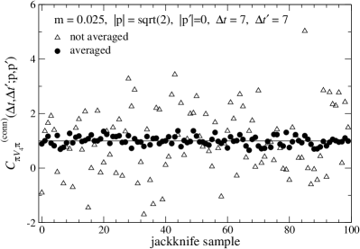
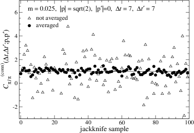
Figure 2: Statistical fluctuation of connected three point functions CπV4π,ϕsϕs(conn)(Δt,Δt;𝐩,𝐩)superscriptsubscript𝐶𝜋subscript𝑉4𝜋subscriptitalic-ϕ𝑠subscriptitalic-ϕ𝑠connΔ𝑡Δsuperscript𝑡𝐩superscript𝐩C_{\pi V_{4}\pi,\phi_{s}\phi_{s}}^{{\rm(conn)}}(\Delta t,\Delta t^{\prime};{\bf p},{\bf p}^{\prime}) (left panel) and Cπ1π,ϕsϕs(conn)(Δt,Δt;𝐩,𝐩)superscriptsubscript𝐶𝜋1𝜋subscriptitalic-ϕ𝑠subscriptitalic-ϕ𝑠connΔ𝑡Δsuperscript𝑡𝐩superscript𝐩C_{\pi 1\pi,\phi_{s}\phi_{s}}^{{\rm(conn)}}(\Delta t,\Delta t^{\prime};{\bf p},{\bf p}^{\prime}) (right panel) with Δt=Δt=7Δ𝑡Δsuperscript𝑡7\Delta t\!=\!\Delta t^{\prime}\!=\!7, |𝐩|=2𝐩2|{\bf p}|\!=\!\sqrt{2} and |𝐩|=0superscript𝐩0|{\bf p}^{\prime}|\!=\!0. Open triangles are jackknife data with a single choice of the source location (𝐱,t)𝐱𝑡({\bf x},t) and momentum configuration (𝐩,𝐩)𝐩superscript𝐩({\bf p},{\bf p}^{\prime}), whereas the filled squares are averaged over (𝐱,t)𝐱𝑡({\bf x},t) and (𝐩,𝐩)𝐩superscript𝐩({\bf p},{\bf p}^{\prime}) corresponding to the same value of q2superscript𝑞2q^{2}. Each data is normalized by its statistical average.

The use of the all-to-all propagator also improves the statistical accuracy of the pion correlators by averaging over the locations of source operator*** We note in passing that only the low-mode contribution is averaged over the locations of the source operator in the so-called low-mode averaging (LMA) method LMA:1 ; LMA:2 . The high-mode contribution in LMA is estimated for a fixed source location using the point-to-all propagator in contrast to our method with the all-to-all propagator. , namely (𝐱,t)𝐱𝑡({\bf x},t) in Eqs. (16) – (19), as well as over momentum configurations (𝐩,𝐩)𝐩superscript𝐩({\bf p},{\bf p}^{\prime}) corresponding to the same value of q2superscript𝑞2q^{2}. Figure 2 compares the statistical fluctuation of connected pion correlators with a certain choice of ΔtΔ𝑡\Delta t, ΔtΔsuperscript𝑡\Delta t^{\prime} and q2superscript𝑞2q^{2}. We observe that averaging over the source locations and momentum configurations remarkably reduces the statistical error of the correlators and leads to very accurate results for the form factors.

III Determination of pion form factors

III.1 Ratio method for vector form factor

In the limit of large temporal separations among pion operators and vector current, two- and three-point functions are dominated by the contribution from the ground state

Cππ,ϕϕ(Δt;𝐩)subscript𝐶𝜋𝜋italic-ϕsuperscriptitalic-ϕΔ𝑡𝐩\displaystyle C_{\pi\pi,\phi\phi^{\prime}}(\Delta t;{\bf p}) ΔtΔ𝑡absent\displaystyle\xrightarrow[\Delta t\to\infty]{} Zπ,ϕ(|𝐩|)Zπ,ϕ(|𝐩|)2Eπ(|𝐩|)eEπ(|𝐩|)Δt,subscript𝑍𝜋superscriptitalic-ϕsuperscript𝐩subscript𝑍𝜋italic-ϕ𝐩2subscript𝐸𝜋𝐩superscript𝑒subscript𝐸𝜋𝐩Δ𝑡\displaystyle\frac{Z_{\pi,\phi^{\prime}}(|{\bf p}|)^{*}\,Z_{\pi,\phi}(|{\bf p}|)}{2\,E_{\pi}(|{\bf p}|)}\,e^{-E_{\pi}(|{\bf p}|)\,\Delta t}, (20)
CπΓπ(conn)(Δt,Δt;𝐩,𝐩)superscriptsubscript𝐶𝜋Γ𝜋connΔ𝑡Δsuperscript𝑡𝐩superscript𝐩\displaystyle C_{\pi\Gamma\pi}^{\rm(conn)}(\Delta t,\Delta t^{\prime};{\bf p},{\bf p}^{\prime}) Δt,ΔtΔ𝑡Δsuperscript𝑡absent\displaystyle\xrightarrow[\Delta t,\Delta t^{\prime}\to\infty]{} Zπ,ϕ(|𝐩|)Zπ,ϕ(|𝐩|)4Eπ(|𝐩|)Eπ(|𝐩|)1ZVπ(p)|Vμ|π(p)subscript𝑍𝜋superscriptitalic-ϕsuperscriptsuperscript𝐩subscript𝑍𝜋italic-ϕ𝐩4subscript𝐸𝜋superscript𝐩subscript𝐸𝜋𝐩1subscript𝑍𝑉quantum-operator-product𝜋superscript𝑝subscript𝑉𝜇𝜋𝑝\displaystyle\frac{Z_{\pi,\phi^{\prime}}(|{\bf p}^{\prime}|)^{*}\,Z_{\pi,\phi}(|{\bf p}|)}{4\,E_{\pi}(|{\bf p}^{\prime}|)E_{\pi}(|{\bf p}|)}\frac{1}{Z_{V}}\langle\pi(p^{\prime})|V_{\mu}|\pi(p)\rangle\, (21)
×eEπ(|𝐩|)ΔteEπ(|𝐩|)Δt,absentsuperscript𝑒subscript𝐸𝜋superscript𝐩Δsuperscript𝑡superscript𝑒subscript𝐸𝜋𝐩Δ𝑡\displaystyle\hskip 113.81102pt\times e^{-E_{\pi}(|{\bf p}^{\prime}|)\,\Delta t^{\prime}}e^{-E_{\pi}(|{\bf p}|)\,\Delta t},

where Zπ,ϕ(|𝐩|)=π(p)|𝒪γ5,ϕsubscript𝑍𝜋italic-ϕ𝐩inner-product𝜋𝑝subscript𝒪subscript𝛾5italic-ϕZ_{\pi,\phi}(|{\bf p}|)\!=\!\langle\pi(p)|{\mathcal{O}}_{\gamma_{5},\phi}\rangle is the overlap of the interpolating field 𝒪γ5,ϕsubscript𝒪subscript𝛾5italic-ϕ{\mathcal{O}}_{\gamma_{5},\phi} to the physical state, and ZVsubscript𝑍𝑉Z_{V} is the renormalization factor for the vector current. For a precise determination of the matrix element π(p)|Vμ|π(p)quantum-operator-product𝜋superscript𝑝subscript𝑉𝜇𝜋𝑝\langle\pi(p^{\prime})|V_{\mu}|\pi(p)\rangle, it is advantageous to take a ratio of appropriately chosen correlators in order to cancel out the exponential damping factors eEπ(|𝐩()|)Δt()superscript𝑒subscript𝐸𝜋superscript𝐩Δsuperscript𝑡e^{-E_{\pi}(|{\bf p}^{(\prime)}|)\Delta t^{(\prime)}} and other unnecessary factors Zπ,ϕ()subscript𝑍𝜋superscriptitalic-ϕZ_{\pi,\phi^{(\prime)}} and ZVsubscript𝑍𝑉Z_{V} dble_ratio . In this study, we use the following ratio to calculate an effective value of the vector form factor FV(q2)subscript𝐹𝑉superscript𝑞2F_{V}(q^{2})

FV(Δt,Δt;q2)subscript𝐹𝑉Δ𝑡Δsuperscript𝑡superscript𝑞2\displaystyle F_{V}(\Delta t,\Delta t^{\prime};q^{2}) =\displaystyle= 2MπEπ(|𝐩|)+Eπ(|𝐩|)RV(Δt,Δt;|𝐩|,|𝐩|,q2)RV(Δt,Δt;0,0,0),2subscript𝑀𝜋subscript𝐸𝜋𝐩subscript𝐸𝜋superscript𝐩subscript𝑅𝑉Δ𝑡Δsuperscript𝑡𝐩superscript𝐩superscript𝑞2subscript𝑅𝑉Δ𝑡Δsuperscript𝑡000\displaystyle\frac{2\,M_{\pi}}{E_{\pi}(|{\bf p}|)+E_{\pi}(|{\bf p}^{\prime}|)}\frac{R_{V}(\Delta t,\Delta t^{\prime};|{\bf p}|,|{\bf p}^{\prime}|,q^{2})}{R_{V}(\Delta t,\Delta t^{\prime};0,0,0)}, (22)
RV(Δt,Δt;|𝐩|,|𝐩|,q2)subscript𝑅𝑉Δ𝑡Δsuperscript𝑡𝐩superscript𝐩superscript𝑞2\displaystyle R_{V}(\Delta t,\Delta t^{\prime};|{\bf p}|,|{\bf p}^{\prime}|,q^{2}) =\displaystyle= 1N|𝐩|,|𝐩|fixed |𝐩|,|𝐩|Cπγ4π(conn)(Δt,Δt;𝐩,𝐩)Cππ,ϕsϕl(Δt;𝐩)Cππ,ϕlϕs(Δt;𝐩),1subscript𝑁𝐩superscript𝐩subscriptfixed 𝐩superscript𝐩superscriptsubscript𝐶𝜋subscript𝛾4𝜋connΔ𝑡Δsuperscript𝑡𝐩superscript𝐩subscript𝐶𝜋𝜋subscriptitalic-ϕ𝑠subscriptitalic-ϕ𝑙Δ𝑡𝐩subscript𝐶𝜋𝜋subscriptitalic-ϕ𝑙subscriptitalic-ϕ𝑠Δsuperscript𝑡superscript𝐩\displaystyle\frac{1}{N_{|{\bf p}|,|{\bf p}^{\prime}|}}\sum_{\mbox{\scriptsize fixed }|{\bf p}|,|{\bf p}^{\prime}|}\frac{C_{\pi\gamma_{4}\pi}^{\rm(conn)}(\Delta t,\Delta t^{\prime};{\bf p},{\bf p}^{\prime})}{C_{\pi\pi,\phi_{s}\phi_{l}}(\Delta t;{\bf p})\,C_{\pi\pi,\phi_{l}\phi_{s}}(\Delta t^{\prime};{\bf p}^{\prime})}, (23)

where (1/N|𝐩|,|𝐩|)fixed |𝐩|,|𝐩|1subscript𝑁𝐩superscript𝐩subscriptfixed 𝐩superscript𝐩(1/N_{|{\bf p}|,|{\bf p}^{\prime}|})\sum_{\mbox{\scriptsize fixed }|{\bf p}|,|{\bf p}^{\prime}|} represents the average over momentum configurations corresponding to the same value of q2superscript𝑞2q^{2}.

Refer to caption
Refer to caption
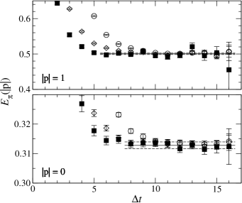
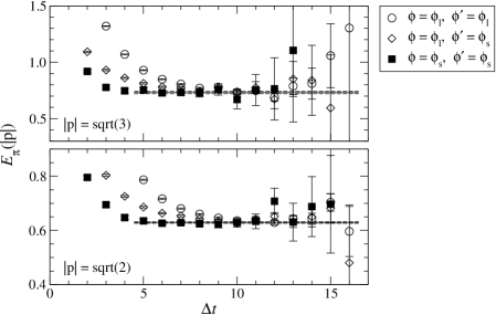
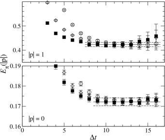
Figure 3: Effective value of pion energy Eπ(|𝐩|)subscript𝐸𝜋𝐩E_{\pi}(|{\bf p}|) at (Q,m)=(0,0.050)𝑄𝑚00.050(Q,m)\!=\!(0,0.050). Circles, triangles and squares show results from Cππ,ϕlϕl(Δt;𝐩)subscript𝐶𝜋𝜋subscriptitalic-ϕ𝑙subscriptitalic-ϕ𝑙Δ𝑡𝐩C_{\pi\pi,\phi_{l}\phi_{l}}(\Delta t;{\bf p}), Cππ,ϕlϕs(Δt;𝐩)subscript𝐶𝜋𝜋subscriptitalic-ϕ𝑙subscriptitalic-ϕ𝑠Δ𝑡𝐩C_{\pi\pi,\phi_{l}\phi_{s}}(\Delta t;{\bf p}) and Cππ,ϕsϕs(Δt;𝐩)subscript𝐶𝜋𝜋subscriptitalic-ϕ𝑠subscriptitalic-ϕ𝑠Δ𝑡𝐩C_{\pi\pi,\phi_{s}\phi_{s}}(\Delta t;{\bf p}), respectively.
Refer to caption
Refer to caption
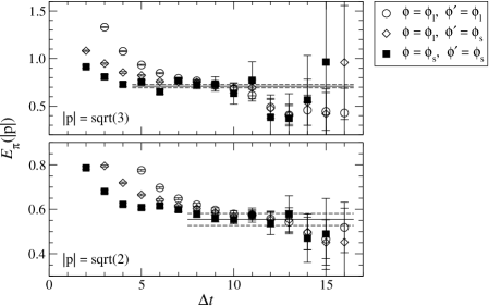
Figure 4: Effective value of pion energy Eπ(|𝐩|)subscript𝐸𝜋𝐩E_{\pi}(|{\bf p}|) at (Q,m)=(0,0.015)𝑄𝑚00.015(Q,m)\!=\!(0,0.015).

The kinematical factor in Eq. (22) involves energies of the initial and final pion states. Effective values of Eπ(|𝐩|)subscript𝐸𝜋𝐩E_{\pi}(|{\bf p}|) at our largest and smallest quark mass are plotted in Figs. 3 and 4. Our data show clear signals up to the largest spatial momentum |𝐩|3𝐩3|{\bf p}|\!\leq\!\sqrt{3}, since their statistical errors are greatly reduced by the use of the all-to-all propagators. We determine Eπ(|𝐩|)subscript𝐸𝜋𝐩E_{\pi}(|{\bf p}|) by a single-cosh fit to Cππ,ϕsϕs(Δt;𝐩)subscript𝐶𝜋𝜋subscriptitalic-ϕ𝑠subscriptitalic-ϕ𝑠Δ𝑡𝐩C_{\pi\pi,\phi_{s}\phi_{s}}(\Delta t;{\bf p}) with a fit range Δt[Δtmin,Nt/2]Δ𝑡Δsubscript𝑡minsubscript𝑁𝑡2\Delta t\in[\Delta t_{\rm min},N_{t}/2]. The minimum temporal separation ΔtminΔsubscript𝑡min\Delta t_{\rm min} is chosen by inspecting ΔtminΔsubscript𝑡min\Delta t_{\rm min} dependence of the fit result. Numerical results for Eπ(|𝐩|)subscript𝐸𝜋𝐩E_{\pi}(|{\bf p}|) are summarized in Table 1. They are consistent with the dispersion relation Eπ(|𝐩|)=Mπ2+𝐩2subscript𝐸𝜋𝐩superscriptsubscript𝑀𝜋2superscript𝐩2E_{\pi}(|{\bf p}|)\!=\!\sqrt{M_{\pi}^{2}+{\bf p}^{2}}, which is commonly assumed in previous studies to estimate Eπ(|𝐩|)subscript𝐸𝜋𝐩E_{\pi}(|{\bf p}|) for |𝐩|>0𝐩0|{\bf p}|\!>\!0. In this work, however, we use the measured value of Eπ(|𝐩|)subscript𝐸𝜋𝐩E_{\pi}(|{\bf p}|) in order not to underestimate uncertainty in Eπ(|𝐩|)subscript𝐸𝜋𝐩E_{\pi}(|{\bf p}|) and hence FV(Δt,Δt;q2)subscript𝐹𝑉Δ𝑡Δsuperscript𝑡superscript𝑞2F_{V}(\Delta t,\Delta t^{\prime};q^{2}).

Table 1: Fit results for pion energy Eπ(|𝐩|)subscript𝐸𝜋𝐩E_{\pi}(|{\bf p}|).
Q𝑄Q m𝑚m |𝐩|=0𝐩0|{\bf p}|\!=\!0 |𝐩|=1𝐩1|{\bf p}|\!=\!1 |𝐩|=2𝐩2|{\bf p}|\!=\!\sqrt{2} |𝐩|=3𝐩3|{\bf p}|\!=\!\sqrt{3}
0 0.015 0.1722(20) 0.4236(88) 0.554(27) 0.710(17)
0 0.025 0.2193(16) 0.4499(58) 0.5791(96) 0.694(16)
0 0.035 0.2610(15) 0.4706(33) 0.6091(59) 0.721(11)
0 0.050 0.3128(12) 0.5005(21) 0.6292(28) 0.732(11)
-2 0.050 0.3124(15) 0.4972(34) 0.6257(67) 0.738(14)
-4 0.050 0.3155(17) 0.4994(29) 0.6353(51) 0.705(10)
Refer to caption
Refer to caption
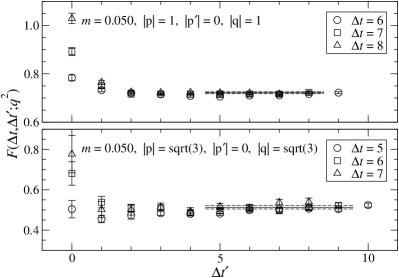
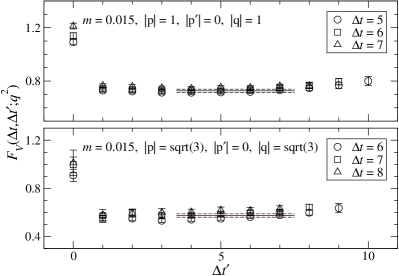
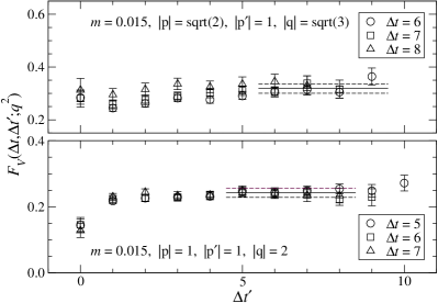
Figure 5: Effective value of vector form factor FV(Δt,Δt;q2)subscript𝐹𝑉Δ𝑡Δsuperscript𝑡superscript𝑞2F_{V}(\Delta t,\Delta t^{\prime};q^{2}) at (Q,m)=(0,0.050)𝑄𝑚00.050(Q,m)\!=\!(0,0.050). We only plot data with Δt+Δt<Nt/2Δ𝑡Δsuperscript𝑡subscript𝑁𝑡2\Delta t\!+\!\Delta t^{\prime}\!<\!N_{t}/2. Momenta written in the legends are spatial and in units of 2πa/L2𝜋𝑎𝐿2\pi a/L.
Refer to caption
Refer to caption
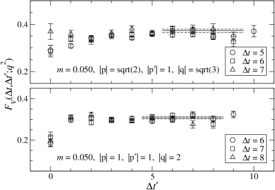
Figure 6: Effective value of FV(Δt,Δt;q2)subscript𝐹𝑉Δ𝑡Δsuperscript𝑡superscript𝑞2F_{V}(\Delta t,\Delta t^{\prime};q^{2}) at (Q,m)=(0,0.015)𝑄𝑚00.015(Q,m)\!=\!(0,0.015).

We extract the vector form factor FV(q2)subscript𝐹𝑉superscript𝑞2F_{V}(q^{2}) by a constant fit to the effective value FV(Δt,Δt;q2)subscript𝐹𝑉Δ𝑡Δsuperscript𝑡superscript𝑞2F_{V}(\Delta t,\Delta t^{\prime};q^{2}). Examples of FV(Δt,Δt;q2)subscript𝐹𝑉Δ𝑡Δsuperscript𝑡superscript𝑞2F_{V}(\Delta t,\Delta t^{\prime};q^{2}) are plotted in Figs. 5 and 6. The all-to-all quark propagator enables us to change ΔtΔ𝑡\Delta t and ΔtΔsuperscript𝑡\Delta t^{\prime} independently in contrast to previous lattice studies with the point-to-all propagator where their sum Δt+ΔtΔ𝑡Δsuperscript𝑡\Delta t\!+\!\Delta t^{\prime} is kept fixed. This is helpful to identify the plateau in FV(Δt,Δt;q2)subscript𝐹𝑉Δ𝑡Δsuperscript𝑡superscript𝑞2F_{V}(\Delta t,\Delta t^{\prime};q^{2}) as well as to stabilize the fit by increasing the number of available data. Fit results are summarized in Tables 2 – 5. The statistical accuracy of FV(q2)subscript𝐹𝑉superscript𝑞2F_{V}(q^{2}) is typically 3 – 5 % at all of our simulated quark masses. Only the combination of our two largest momenta (|𝐩|,|𝐩|)=(3,2)𝐩superscript𝐩32(|{\bf p}|,|{\bf p}^{\prime}|)\!=\!(\sqrt{3},\sqrt{2}) has larger statistical error of about 10 %. This is probably because precise determination of the ground state contribution is difficult due to very rapid damping of pion correlators with such large momenta.

Table 2: Fit results for pion form factors at (Q,m)=(0,0.050)𝑄𝑚00.050(Q,m)\!=\!(0,0.050).
|𝐩|𝐩|{\bf p}| |𝐩|superscript𝐩|{\bf p}^{\prime}| |𝐪|𝐪|{\bf q}| q2superscript𝑞2q^{2} FV(q2)subscript𝐹𝑉superscript𝑞2F_{V}(q^{2}) FS(q2)FS(qref2)subscript𝐹𝑆superscript𝑞2subscript𝐹𝑆superscriptsubscript𝑞ref2\frac{F_{S}(q^{2})}{F_{S}(q_{\rm ref}^{2})} |𝐩|𝐩|{\bf p}| |𝐩|superscript𝐩|{\bf p}^{\prime}| |𝐪|𝐪|{\bf q}| q2superscript𝑞2q^{2} FV(q2)subscript𝐹𝑉superscript𝑞2F_{V}(q^{2}) FS(q2)FS(qref2)subscript𝐹𝑆superscript𝑞2subscript𝐹𝑆superscriptsubscript𝑞ref2\frac{F_{S}(q^{2})}{F_{S}(q_{\rm ref}^{2})}
00 00 00 0 1 1.30(11) 33\sqrt{3} 00 33\sqrt{3} -0.2865(95) 0.5132(83) 0.705(44)
111 00 111 -0.1190(7) 0.7219(37) 33\sqrt{3} 111 22\sqrt{2} -0.2546(51) 0.522(17) 0.728(66)
22\sqrt{2} 111 111 -0.13763(68) 0.660(13) 0.918(37) 111 111 22\sqrt{2} -0.3084(0) 0.4755(47) 0.759(21)
33\sqrt{3} 22\sqrt{2} 111 -0.1436(23) 0.599(49) 0.907(90) 22\sqrt{2} 111 33\sqrt{3} -0.4461(7) 0.3726(72) 0.681(34)
22\sqrt{2} 00 22\sqrt{2} -0.2083(18) 0.5908(45) 0.871(17) 111 111 222 -0.6169(0) 0.3075(61) 0.605(33)
Table 3: Fit results for pion form factors at (Q,m)=(0,0.035)𝑄𝑚00.035(Q,m)\!=\!(0,0.035).
|𝐩|𝐩|{\bf p}| |𝐩|superscript𝐩|{\bf p}^{\prime}| |𝐪|𝐪|{\bf q}| q2superscript𝑞2q^{2} FV(q2)subscript𝐹𝑉superscript𝑞2F_{V}(q^{2}) FS(q2)FS(qref2)subscript𝐹𝑆superscript𝑞2subscript𝐹𝑆superscriptsubscript𝑞ref2\frac{F_{S}(q^{2})}{F_{S}(q_{\rm ref}^{2})} |𝐩|𝐩|{\bf p}| |𝐩|superscript𝐩|{\bf p}^{\prime}| |𝐪|𝐪|{\bf q}| q2superscript𝑞2q^{2} FV(q2)subscript𝐹𝑉superscript𝑞2F_{V}(q^{2}) FS(q2)FS(qref2)subscript𝐹𝑆superscript𝑞2subscript𝐹𝑆superscriptsubscript𝑞ref2\frac{F_{S}(q^{2})}{F_{S}(q_{\rm ref}^{2})}
00 00 00 0 1 1.28(10) 33\sqrt{3} 00 33\sqrt{3} -0.2513(99) 0.5266(98) 0.673(69)
111 00 111 -0.1103(15) 0.7272(65) 33\sqrt{3} 111 22\sqrt{2} -0.2459(54) 0.513(25) 0.783(66)
22\sqrt{2} 111 111 -0.1350(17) 0.638(18) 0.902(43) 111 111 22\sqrt{2} -0.3084(0) 0.4518(80) 0.765(27)
33\sqrt{3} 22\sqrt{2} 111 -0.1417(27) 0.610(85) 0.890(87) 22\sqrt{2} 111 33\sqrt{3} -0.4435(17) 0.358(11) 0.648(53)
22\sqrt{2} 00 22\sqrt{2} -0.1873(44) 0.5964(75) 0.728(64) 111 111 222 -0.6169(0) 0.2882(76) 0.546(31)
Table 4: Fit results for pion form factors at (Q,m)=(0,0.025)𝑄𝑚00.025(Q,m)\!=\!(0,0.025).
|𝐩|𝐩|{\bf p}| |𝐩|superscript𝐩|{\bf p}^{\prime}| |𝐪|𝐪|{\bf q}| q2superscript𝑞2q^{2} FV(q2)subscript𝐹𝑉superscript𝑞2F_{V}(q^{2}) FS(q2)FS(qref2)subscript𝐹𝑆superscript𝑞2subscript𝐹𝑆superscriptsubscript𝑞ref2\frac{F_{S}(q^{2})}{F_{S}(q_{\rm ref}^{2})} |𝐩|𝐩|{\bf p}| |𝐩|superscript𝐩|{\bf p}^{\prime}| |𝐪|𝐪|{\bf q}| q2superscript𝑞2q^{2} FV(q2)subscript𝐹𝑉superscript𝑞2F_{V}(q^{2}) FS(q2)FS(qref2)subscript𝐹𝑆superscript𝑞2subscript𝐹𝑆superscriptsubscript𝑞ref2\frac{F_{S}(q^{2})}{F_{S}(q_{\rm ref}^{2})}
00 00 00 0 1 1.29(13) 33\sqrt{3} 00 33\sqrt{3} -0.237(15) 0.529(12) 0.650(35)
111 00 111 -0.1010(27) 0.7327(88) 33\sqrt{3} 111 22\sqrt{2} -0.2489(83) 0.474(24) 0.56(11)
22\sqrt{2} 111 111 -0.1375(27) 0.627(21) 0.939(61) 111 111 22\sqrt{2} -0.3084(0) 0.422(11) 0.686(42)
33\sqrt{3} 22\sqrt{2} 111 -0.1410(38) 0.550(60) 0.49(31) 22\sqrt{2} 111 33\sqrt{3} -0.4460(27) 0.337(12) 0.548(50)
22\sqrt{2} 00 22\sqrt{2} -0.1790(70) 0.600(10) 0.768(30) 111 111 222 -0.6169(0) 0.2561(87) 0.523(54)
Table 5: Fit results for pion form factors at (Q,m)=(0,0.015)𝑄𝑚00.015(Q,m)\!=\!(0,0.015).
|𝐩|𝐩|{\bf p}| |𝐩|superscript𝐩|{\bf p}^{\prime}| |𝐪|𝐪|{\bf q}| q2superscript𝑞2q^{2} FV(q2)subscript𝐹𝑉superscript𝑞2F_{V}(q^{2}) FS(q2)FS(qref2)subscript𝐹𝑆superscript𝑞2subscript𝐹𝑆superscriptsubscript𝑞ref2\frac{F_{S}(q^{2})}{F_{S}(q_{\rm ref}^{2})} |𝐩|𝐩|{\bf p}| |𝐩|superscript𝐩|{\bf p}^{\prime}| |𝐪|𝐪|{\bf q}| q2superscript𝑞2q^{2} FV(q2)subscript𝐹𝑉superscript𝑞2F_{V}(q^{2}) FS(q2)FS(qref2)subscript𝐹𝑆superscript𝑞2subscript𝐹𝑆superscriptsubscript𝑞ref2\frac{F_{S}(q^{2})}{F_{S}(q_{\rm ref}^{2})}
00 00 00 0 1 1.29(19) 33\sqrt{3} 00 33\sqrt{3} -0.174(18) 0.574(14) 0.621(90)
111 00 111 -0.0910(44) 0.727(13) 33\sqrt{3} 111 22\sqrt{2} -0.227(11) 0.484(33) 0.80(12)
22\sqrt{2} 111 111 -0.1372(73) 0.645(34) 0.926(86) 111 111 22\sqrt{2} -0.3084(0) 0.403(16) 0.643(95)
33\sqrt{3} 22\sqrt{2} 111 -0.1301(98) 0.629(74) 0.81(41) 22\sqrt{2} 111 33\sqrt{3} -0.4456(73) 0.319(18) 0.599(81)
22\sqrt{2} 00 22\sqrt{2} -0.162(21) 0.631(25) 0.805(44) 111 111 222 -0.6169(0) 0.242(14) 0.65(13)
Refer to caption
Refer to caption
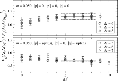
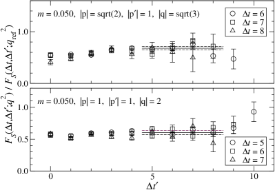
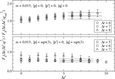
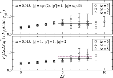
Figure 7: Effective value of normalized scalar form factor FS(Δt,Δt;q2)/FS(Δt,Δt;qref2)subscript𝐹𝑆Δ𝑡Δsuperscript𝑡superscript𝑞2subscript𝐹𝑆Δ𝑡Δsuperscript𝑡superscriptsubscript𝑞ref2F_{S}(\Delta t,\Delta t^{\prime};q^{2})/F_{S}(\Delta t,\Delta t^{\prime};q_{\rm ref}^{2}) at (Q,m)=(0,0.050)𝑄𝑚00.050(Q,m)\!=\!(0,0.050).
Refer to caption
Refer to caption
Figure 8: Effective value of FS(Δt,Δt;q2)/FS(Δt,Δt;qref2)subscript𝐹𝑆Δ𝑡Δsuperscript𝑡superscript𝑞2subscript𝐹𝑆Δ𝑡Δsuperscript𝑡superscriptsubscript𝑞ref2F_{S}(\Delta t,\Delta t^{\prime};q^{2})/F_{S}(\Delta t,\Delta t^{\prime};q_{\rm ref}^{2}) at (Q,m)=(0,0.015)𝑄𝑚00.015(Q,m)\!=\!(0,0.015).

III.2 Scalar form factor

The scalar form factor normalized by the value at a certain momentum transfer qref2superscriptsubscript𝑞ref2q_{\rm ref}^{2} can be calculated from the following ratio similar to that for FV(q2)subscript𝐹𝑉superscript𝑞2F_{V}(q^{2})

FS(Δt,Δt;q2)FS(Δt,Δt;qref2)subscript𝐹𝑆Δ𝑡Δsuperscript𝑡superscript𝑞2subscript𝐹𝑆Δ𝑡Δsuperscript𝑡superscriptsubscript𝑞ref2\displaystyle\frac{F_{S}(\Delta t,\Delta t^{\prime};q^{2})}{F_{S}(\Delta t,\Delta t^{\prime};q_{\rm ref}^{2})} =\displaystyle= RS(Δt,Δt;q2)RS(Δt,Δt;qref2),subscript𝑅𝑆Δ𝑡Δsuperscript𝑡superscript𝑞2subscript𝑅𝑆Δ𝑡Δsuperscript𝑡superscriptsubscript𝑞ref2\displaystyle\frac{R_{S}(\Delta t,\Delta t^{\prime};q^{2})}{R_{S}(\Delta t,\Delta t^{\prime};q_{\rm ref}^{2})}, (24)
RS(Δt,Δt;q2)subscript𝑅𝑆Δ𝑡Δsuperscript𝑡superscript𝑞2\displaystyle R_{S}(\Delta t,\Delta t^{\prime};q^{2}) =\displaystyle= 1N|𝐩|,|𝐩|fixed |𝐩|,|𝐩|Cπ1π(sngl)(Δt,Δt;𝐩,𝐩)Cππ,ϕsϕl(Δt;𝐩)Cππ,ϕlϕs(Δt;𝐩),1subscript𝑁𝐩superscript𝐩subscriptfixed 𝐩superscript𝐩superscriptsubscript𝐶𝜋1𝜋snglΔ𝑡Δsuperscript𝑡𝐩superscript𝐩subscript𝐶𝜋𝜋subscriptitalic-ϕ𝑠subscriptitalic-ϕ𝑙Δ𝑡𝐩subscript𝐶𝜋𝜋subscriptitalic-ϕ𝑙subscriptitalic-ϕ𝑠Δsuperscript𝑡superscript𝐩\displaystyle\frac{1}{N_{|{\bf p}|,|{\bf p}^{\prime}|}}\sum_{\mbox{\scriptsize fixed }|{\bf p}|,|{\bf p}^{\prime}|}\frac{C_{\pi 1\pi}^{\rm(sngl)}(\Delta t,\Delta t^{\prime};{\bf p},{\bf p}^{\prime})}{C_{\pi\pi,\phi_{s}\phi_{l}}(\Delta t;{\bf p})\,C_{\pi\pi,\phi_{l}\phi_{s}}(\Delta t^{\prime};{\bf p}^{\prime})}, (25)

where

Cπ1π(sngl)(Δt,Δt;𝐩,𝐩)superscriptsubscript𝐶𝜋1𝜋snglΔ𝑡Δsuperscript𝑡𝐩superscript𝐩\displaystyle C_{\pi 1\pi}^{\rm(sngl)}(\Delta t,\Delta t^{\prime};{\bf p},{\bf p}^{\prime}) =\displaystyle= Cπ1π(conn)(Δt,Δt;𝐩,𝐩)Cπ1π(disc)(Δt,Δt;𝐩,𝐩)superscriptsubscript𝐶𝜋1𝜋connΔ𝑡Δsuperscript𝑡𝐩superscript𝐩superscriptsubscript𝐶𝜋1𝜋discΔ𝑡Δsuperscript𝑡𝐩superscript𝐩\displaystyle C_{\pi 1\pi}^{\rm(conn)}(\Delta t,\Delta t^{\prime};{\bf p},{\bf p}^{\prime})-C_{\pi 1\pi}^{\rm(disc)}(\Delta t,\Delta t^{\prime};{\bf p},{\bf p}^{\prime})
+Cπ1π(vev)(Δt,Δt;𝐩,𝐩)superscriptsubscript𝐶𝜋1𝜋vevΔ𝑡Δsuperscript𝑡𝐩superscript𝐩\displaystyle\hskip 103.85255pt+\,C_{\pi 1\pi}^{\rm(vev)}(\Delta t,\Delta t^{\prime};{\bf p},{\bf p}^{\prime})

is the three-point function with the flavor-singlet scalar operator. We note that Cπ1π(disc)Cπ1π(vev)superscriptsubscript𝐶𝜋1𝜋discsuperscriptsubscript𝐶𝜋1𝜋vevC_{\pi 1\pi}^{\rm(disc)}\!-\!C_{\pi 1\pi}^{\rm(vev)} suffers from a severe cancellation: it is typically a subtraction of O(1)𝑂1O(1) quantities to extract their O(103)𝑂superscript103O(10^{-3}) difference. Although this subtraction leads to a large statistical error in FS(q2)subscript𝐹𝑆superscript𝑞2F_{S}(q^{2}), it is present only at |𝐪|=0𝐪0|{\bf q}|\!=\!0, since Cπ1π(vev)superscriptsubscript𝐶𝜋1𝜋vevC_{\pi 1\pi}^{\rm(vev)} vanishes at nonzero |𝐪|𝐪|{\bf q}|. In the following analysis, therefore, we use FS(q2)subscript𝐹𝑆superscript𝑞2F_{S}(q^{2}) normalized at the smallest nonzero |q2|superscript𝑞2|q^{2}| with |𝐪ref|=1subscript𝐪ref1|{\bf q}_{\rm ref}|\!=\!1 rather than at q2=0superscript𝑞20q^{2}\!=\!0. The effective value of the normalized scalar form factor FS(Δt,Δt;q2)/FS(Δt,Δt;qref2)subscript𝐹𝑆Δ𝑡Δsuperscript𝑡superscript𝑞2subscript𝐹𝑆Δ𝑡Δsuperscript𝑡superscriptsubscript𝑞ref2F_{S}(\Delta t,\Delta t^{\prime};q^{2})/F_{S}(\Delta t,\Delta t^{\prime};q_{\rm ref}^{2}) is plotted in Figs. 7 and 8. We summarize FS(q2)/FS(qref2)subscript𝐹𝑆superscript𝑞2subscript𝐹𝑆superscriptsubscript𝑞ref2F_{S}(q^{2})/F_{S}(q_{\rm ref}^{2}) determined from a constant fit to FS(Δt,Δt;q2)/FS(Δt,Δt;qref2)subscript𝐹𝑆Δ𝑡Δsuperscript𝑡superscript𝑞2subscript𝐹𝑆Δ𝑡Δsuperscript𝑡superscriptsubscript𝑞ref2F_{S}(\Delta t,\Delta t^{\prime};q^{2})/F_{S}(\Delta t,\Delta t^{\prime};q_{\rm ref}^{2}) in Tables 2 – 5.

Refer to caption
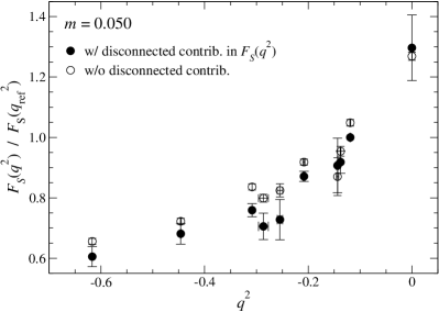
Figure 9: Normalized scalar form factor FS(q2)/FS(qref2)subscript𝐹𝑆superscript𝑞2subscript𝐹𝑆superscriptsubscript𝑞ref2F_{S}(q^{2})/F_{S}(q_{\rm ref}^{2}) with and without the contributions of disconnected diagram to FS(q2)subscript𝐹𝑆superscript𝑞2F_{S}(q^{2}). We use the normalization value FS(qref2)subscript𝐹𝑆superscriptsubscript𝑞ref2F_{S}(q_{\rm ref}^{2}) with the disconnected contributions in both data.

Figure 9 compares FS(q2)/FS(qref2)subscript𝐹𝑆superscript𝑞2subscript𝐹𝑆superscriptsubscript𝑞ref2F_{S}(q^{2})/F_{S}(q_{\rm ref}^{2}) to that without the contributions of the disconnected diagrams to FS(q2)subscript𝐹𝑆superscript𝑞2F_{S}(q^{2}). We observe a small but significant deviation between the two data, which implies the importance of the disconnected contributions.

An accurate estimate of FS(0)subscript𝐹𝑆0F_{S}(0) is useful for a precise determination of the scalar radius r2Ssubscriptdelimited-⟨⟩superscript𝑟2𝑆\langle r^{2}\rangle_{S}, as it characterizes the q2superscript𝑞2q^{2} dependence of FS(q2)subscript𝐹𝑆superscript𝑞2F_{S}(q^{2}) near q2=0superscript𝑞20q^{2}\!=\!0. Since the extraction of FS(0)subscript𝐹𝑆0F_{S}(0) from the three-point function suffers from large statistical error due to the subtraction of the vacuum expectation value (VEV) of the scalar operator, we test an alternative calculation of FS(0)subscript𝐹𝑆0F_{S}(0) through the Feynman-Hellmann theorem

FS(0)subscript𝐹𝑆0\displaystyle F_{S}(0) =\displaystyle= 12Mπ2m,12superscriptsubscript𝑀𝜋2𝑚\displaystyle\frac{1}{2}\frac{\partial M_{\pi}^{2}}{\partial m}, (27)

where the VEV subtraction is implicitly taken into account. Note that the overall factor 1/2 is present in the RHS, since m𝑚m is the mass of two degenerate quark flavors. This and FS(qref)subscript𝐹𝑆subscript𝑞refF_{S}(q_{\rm ref}) determined from a ratio of pion correlators

FS(q2)subscript𝐹𝑆superscript𝑞2\displaystyle F_{S}(q^{2}) Δt,ΔtΔ𝑡Δsuperscript𝑡absent\displaystyle\xleftarrow[\Delta t,\Delta t^{\prime}\to\infty]{} 2ZSEπ(|𝐩|)Cπ1π(sngl)(Δt,Δt;𝐩,𝐩)Cππ,ϕsϕl(Δt;𝐩)Cππ,ϕsϕl(Δt;𝐩)Cππ,ϕsϕs(Δt+Δt;𝐩)2subscript𝑍𝑆subscript𝐸𝜋superscript𝐩superscriptsubscript𝐶𝜋1𝜋snglΔ𝑡Δsuperscript𝑡𝐩superscript𝐩subscript𝐶𝜋𝜋subscriptitalic-ϕ𝑠subscriptitalic-ϕ𝑙Δsuperscript𝑡superscript𝐩subscript𝐶𝜋𝜋subscriptitalic-ϕ𝑠subscriptitalic-ϕ𝑙Δ𝑡𝐩subscript𝐶𝜋𝜋subscriptitalic-ϕ𝑠subscriptitalic-ϕ𝑠Δ𝑡Δsuperscript𝑡superscript𝐩\displaystyle 2Z_{S}E_{\pi}(|{\bf p}^{\prime}|)\frac{C_{\pi 1\pi}^{\rm(sngl)}(\Delta t,\Delta t^{\prime};{\bf p},{\bf p}^{\prime})\,C_{\pi\pi,\phi_{s}\phi_{l}}(\Delta t^{\prime};{\bf p}^{\prime})}{C_{\pi\pi,\phi_{s}\phi_{l}}(\Delta t;{\bf p})\,C_{\pi\pi,\phi_{s}\phi_{s}}(\Delta t+\Delta t^{\prime};{\bf p}^{\prime})} (28)

provide an alternative estimate of the normalized form factor FS(0)/FS(qref2)subscript𝐹𝑆0subscript𝐹𝑆superscriptsubscript𝑞ref2F_{S}(0)/F_{S}(q_{\rm ref}^{2}). We determine FS(0)subscript𝐹𝑆0F_{S}(0) from the chiral fit of Mπ2superscriptsubscript𝑀𝜋2M_{\pi}^{2} and ZS=0.838(14)(3)subscript𝑍𝑆0.838143Z_{S}\!=\!0.838(14)(3) presented in Ref. Spectrum:Nf2:RG+Ovr:JLQCD . Results for FS(0)subscript𝐹𝑆0F_{S}(0) and FS(0)/FS(qref2)subscript𝐹𝑆0subscript𝐹𝑆superscriptsubscript𝑞ref2F_{S}(0)/F_{S}(q_{\rm ref}^{2}) are summarized in Table 6, where the systematic error is estimated by changing the fitting form for Mπ2superscriptsubscript𝑀𝜋2M_{\pi}^{2} and by taking account of the uncertainty in ZSsubscript𝑍𝑆Z_{S}. It turns out that, with the setup of our measurements, the Feynman-Hellmann theorem (27) leads to a slightly smaller uncertainty in FS(0)/FS(qref2)subscript𝐹𝑆0subscript𝐹𝑆superscriptsubscript𝑞ref2F_{S}(0)/F_{S}(q_{\rm ref}^{2}) than that from the ratio (24). We therefore adopt FS(0)/FS(qref2)subscript𝐹𝑆0subscript𝐹𝑆superscriptsubscript𝑞ref2F_{S}(0)/F_{S}(q_{\rm ref}^{2}) in Table 6 and FS(q20)/FS(qref2)subscript𝐹𝑆superscript𝑞20subscript𝐹𝑆superscriptsubscript𝑞ref2F_{S}(q^{2}\!\neq\!0)/F_{S}(q_{\rm ref}^{2}) in Tables 2 – 5 in the following analysis.

Table 6: Scalar form factor FS(0)subscript𝐹𝑆0F_{S}(0) determined from Feynman-Hellmann theorem Eq. (27), and its value normalized by FS(qref2)subscript𝐹𝑆superscriptsubscript𝑞ref2F_{S}(q_{\rm ref}^{2}) from ratio (28). The first error is statistical. The second is systematics due to the choice of the fit form for Mπ2superscriptsubscript𝑀𝜋2M_{\pi}^{2} and uncertainty in ZSsubscript𝑍𝑆Z_{S}.
m𝑚m 0.015 0.025 0.035 0.050
FS(0)subscript𝐹𝑆0F_{S}(0) 1.149(6)(22) 1.162(18)(37) 1.208(29)(47) 1.319(44)(52)
FS(0)/FS(qref2)subscript𝐹𝑆0subscript𝐹𝑆superscriptsubscript𝑞ref2F_{S}(0)/F_{S}(q_{\rm ref}^{2}) 1.413(70)(28) 1.415(44)(44) 1.338(38)(51) 1.441(53)(58)

III.3 Finite volume correction

The finite volume effect could be significant at two smallest quark masses m=0.015𝑚0.015m\!=\!0.015 and 0.025, as the value of MπLsubscript𝑀𝜋𝐿M_{\pi}\,L is less than 4. We estimate the finite volume correction (FVC) to the pion mass as presented in Ref. Spectrum:Nf2:RG+Ovr:JLQCD . The FVC to the vector form factor FV(q2)subscript𝐹𝑉superscript𝑞2F_{V}(q^{2}) has been calculated within one-loop ChPT in Refs. FVC:PFF:V:ChPT ; FVC:PFF:V:LChPT by replacing the loop integral by a discrete sum

ΔFV(q2)Δsubscript𝐹𝑉superscript𝑞2\displaystyle\Delta F_{V}(q^{2}) =\displaystyle= 12F201𝑑x{I1/2(L,x𝐪,Mπ2+x(1x)q2)I1/2(L,𝟎,Mπ2)},12superscript𝐹2superscriptsubscript01differential-d𝑥subscript𝐼12𝐿𝑥𝐪superscriptsubscript𝑀𝜋2𝑥1𝑥superscript𝑞2subscript𝐼12𝐿0superscriptsubscript𝑀𝜋2\displaystyle\frac{1}{2F^{2}}\int_{0}^{1}dx\left\{I_{1/2}(L,x{\bf q},M_{\pi}^{2}+x(1-x)q^{2})-I_{1/2}(L,{\bf 0},M_{\pi}^{2})\right\}, (29)

where

Is(L,Δ𝐤,M2)subscript𝐼𝑠𝐿Δ𝐤superscript𝑀2\displaystyle I_{s}(L,\Delta{\bf k},M^{2}) =\displaystyle= d3k(2π)31{(𝐤+Δ𝐤)2+M2}s1L3𝐤1{(𝐤+Δ𝐤)2+M2}s.superscript𝑑3𝑘superscript2𝜋31superscriptsuperscript𝐤Δ𝐤2superscript𝑀2𝑠1superscript𝐿3subscript𝐤1superscriptsuperscript𝐤Δ𝐤2superscript𝑀2𝑠\displaystyle\int\frac{d^{3}k}{(2\pi)^{3}}\frac{1}{\left\{({\bf k}+\Delta{\bf k})^{2}+M^{2}\right\}^{s}}-\frac{1}{L^{3}}\sum_{{\bf k}}\frac{1}{\left\{({\bf k}+\Delta{\bf k})^{2}+M^{2}\right\}^{s}}. (30)

This function can be evaluated through the elliptic θ𝜃\theta function FVC:PFF:V:Is:1 ; FVC:PFF:V:Is:2 as

Is(L,Δ𝐤,M2)subscript𝐼𝑠𝐿Δ𝐤superscript𝑀2\displaystyle I_{s}(L,\Delta{\bf k},M^{2}) =\displaystyle= 1(4π)3/2Γ(s)0𝑑ττs5/2eM2τ{1i=13θ3(L2Δki,eL2/4τ)},1superscript4𝜋32Γ𝑠superscriptsubscript0differential-d𝜏superscript𝜏𝑠52superscript𝑒superscript𝑀2𝜏1superscriptsubscriptproduct𝑖13subscript𝜃3𝐿2Δsubscript𝑘𝑖superscript𝑒superscript𝐿24𝜏\displaystyle\frac{1}{(4\pi)^{3/2}\Gamma(s)}\int_{0}^{\infty}d\tau\tau^{s-5/2}e^{-M^{2}\tau}\left\{1-\prod_{i=1}^{3}\theta_{3}\left(\frac{L}{2}\Delta k_{i},e^{-L^{2}/4\tau}\right)\right\}, (31)
θ3(u,q)subscript𝜃3𝑢𝑞\displaystyle\theta_{3}(u,q) =\displaystyle= n=qn2e2nui.superscriptsubscript𝑛superscript𝑞superscript𝑛2superscript𝑒2𝑛𝑢𝑖\displaystyle\sum_{n=-\infty}^{\infty}q^{n^{2}}e^{2nui}. (32)

The FVC to the scalar form factor FS(q2)subscript𝐹𝑆superscript𝑞2F_{S}(q^{2}) is similarly evaluated as

ΔFS(q2)Δsubscript𝐹𝑆superscript𝑞2\displaystyle\Delta F_{S}(q^{2}) =\displaystyle= B2F201𝑑x{2q2+Mπ22I3/2(L,x𝐪,Mπ2+x(1x)q2)+I1/2(L,𝟎,Mπ2)},𝐵2superscript𝐹2superscriptsubscript01differential-d𝑥2superscript𝑞2superscriptsubscript𝑀𝜋22subscript𝐼32𝐿𝑥𝐪superscriptsubscript𝑀𝜋2𝑥1𝑥superscript𝑞2subscript𝐼12𝐿0superscriptsubscript𝑀𝜋2\displaystyle\frac{B}{2F^{2}}\int_{0}^{1}dx\left\{-\frac{2q^{2}+M_{\pi}^{2}}{2}I_{3/2}(L,x{\bf q},M_{\pi}^{2}+x(1-x)q^{2})+I_{1/2}(L,{\bf 0},M_{\pi}^{2})\right\}, (33)

where we use B=2.10(45)𝐵2.1045B\!=\!2.10(45) GeV obtained from our analysis of the pion mass Spectrum:Nf2:RG+Ovr:JLQCD . We find that ΔFV(q2)Δsubscript𝐹𝑉superscript𝑞2\Delta F_{V}(q^{2}) has a mild q2superscript𝑞2q^{2} dependence and its magnitude is similar to or smaller than the statistical error: it is typically 3 – 5 % at m=0.015𝑚0.015m\!=\!0.015, and decreases down to 1less-than-or-similar-toabsent1\lesssim 1 % at m=0.050𝑚0.050m\!=\!0.050. The FVC to the normalized scalar form factor FS(q2)/FS(qref2)subscript𝐹𝑆superscript𝑞2subscript𝐹𝑆superscriptsubscript𝑞ref2F_{S}(q^{2})/F_{S}(q_{\rm ref}^{2}) is below the statistical uncertainty even at our smallest quark mass due to a partial cancellation of FVCs in the ratio. We use FV(q2)subscript𝐹𝑉superscript𝑞2F_{V}(q^{2}) and FS(q2)/FS(qref2)subscript𝐹𝑆superscript𝑞2subscript𝐹𝑆superscriptsubscript𝑞ref2F_{S}(q^{2})/F_{S}(q_{\rm ref}^{2}) with the FVC included in the following analysis.
Refer to caption
Refer to caption
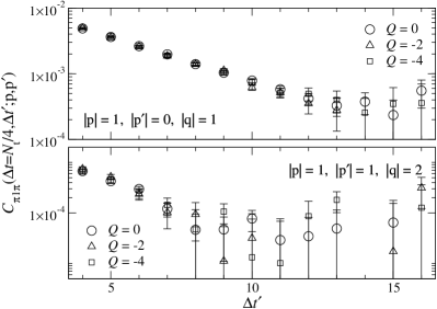
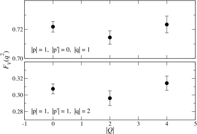
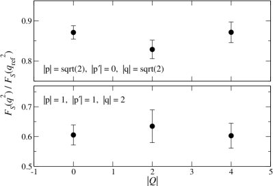
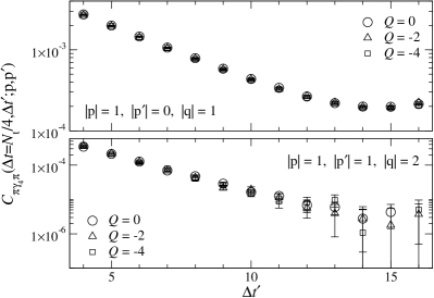
Figure 10: Three-point functions with vector current (left panels) and scalar operator (right panels) calculated in different topological sectors for m=0.050𝑚0.050m\!=\!0.050. Top and bottom panels show data at the smallest and largest nonzero |q2|superscript𝑞2|q^{2}|.

III.4 Fixed topology effects

The form factors listed in Tables 2 – 5 are extracted in the trivial topological sector, and are subject to effects of the fixed topology. The effects are known to be suppressed by the inverse space-time volume 1/V1𝑉1/V fixed_Q:BCNW ; fixed_Q:AFHO , and are systematically correctable fixed_Q:AFHO . In order to confirm if the correction to our data is statistically insignificant, we repeat the calculation of FV(q2)subscript𝐹𝑉superscript𝑞2F_{V}(q^{2}) and FS(q2)subscript𝐹𝑆superscript𝑞2F_{S}(q^{2}) in non-trivial topological sectors with Q=2𝑄2Q\!=\!-2 and 44-4 at m=0.050𝑚0.050m\!=\!0.050. Note that, LO ChPT predicts Q2=mΣV/28delimited-⟨⟩superscript𝑄2𝑚Σ𝑉2similar-to8\langle Q^{2}\rangle\!=\!m\Sigma V/2\!\sim\!8 with our estimate of the chiral condensate ΣMS¯(2 GeV)=(0.236(5+14)GeV)3\Sigma^{\scriptsize\overline{\mbox{MS}}}(\mbox{2~{}GeV})\!=\!(0.236(^{+14}_{-5})~{}\mbox{GeV})^{3} Spectrum:Nf2:RG+Ovr:JLQCD . It is therefore not necessary to simulate topological sectors with |Q|Q23much-greater-than𝑄delimited-⟨⟩superscript𝑄2similar-to3|Q|\gg\sqrt{\langle Q^{2}\rangle}\sim 3 at this quark mass.

Table 7: Fit results for pion form factors at (Q,m)=(2,0.050)𝑄𝑚20.050(Q,m)\!=\!(-2,0.050).
|𝐩|𝐩|{\bf p}| |𝐩|superscript𝐩|{\bf p}^{\prime}| |𝐪|𝐪|{\bf q}| q2superscript𝑞2q^{2} FV(q2)subscript𝐹𝑉superscript𝑞2F_{V}(q^{2}) FS(q2)FS(qref2)subscript𝐹𝑆superscript𝑞2subscript𝐹𝑆superscriptsubscript𝑞ref2\frac{F_{S}(q^{2})}{F_{S}(q_{\rm ref}^{2})} |𝐩|𝐩|{\bf p}| |𝐩|superscript𝐩|{\bf p}^{\prime}| |𝐪|𝐪|{\bf q}| q2superscript𝑞2q^{2} FV(q2)subscript𝐹𝑉superscript𝑞2F_{V}(q^{2}) FS(q2)FS(qref2)subscript𝐹𝑆superscript𝑞2subscript𝐹𝑆superscriptsubscript𝑞ref2\frac{F_{S}(q^{2})}{F_{S}(q_{\rm ref}^{2})}
111 00 111 -0.1200(11) 0.7145(46) 33\sqrt{3} 111 22\sqrt{2} -0.2503(70) 0.481(22) 0.79(13)
22\sqrt{2} 111 111 -0.1377(15) 0.667(20) 0.923(51) 111 111 22\sqrt{2} -0.3084(0) 0.4640(65) 0.738(29)
33\sqrt{3} 22\sqrt{2} 111 -0.1416(33) 0.662(56) 0.32(34) 22\sqrt{2} 111 33\sqrt{3} -0.4461(15) 0.365(11) 0.694(46)
22\sqrt{2} 00 22\sqrt{2} -0.2102(40) 0.5910(75) 0.829(23) 111 111 222 -0.6169(0) 0.2962(89) 0.635(55)
33\sqrt{3} 00 33\sqrt{3} -0.281(12) 0.5113(97) 0.785(65)
Table 8: Fit results for pion form factors at (Q,m)=(4,0.050)𝑄𝑚40.050(Q,m)\!=\!(-4,0.050).
|𝐩|𝐩|{\bf p}| |𝐩|superscript𝐩|{\bf p}^{\prime}| |𝐪|𝐪|{\bf q}| q2superscript𝑞2q^{2} FV(q2)subscript𝐹𝑉superscript𝑞2F_{V}(q^{2}) FS(q2)FS(qref2)subscript𝐹𝑆superscript𝑞2subscript𝐹𝑆superscriptsubscript𝑞ref2\frac{F_{S}(q^{2})}{F_{S}(q_{\rm ref}^{2})} |𝐩|𝐩|{\bf p}| |𝐩|superscript𝐩|{\bf p}^{\prime}| |𝐪|𝐪|{\bf q}| q2superscript𝑞2q^{2} FV(q2)subscript𝐹𝑉superscript𝑞2F_{V}(q^{2}) FS(q2)FS(qref2)subscript𝐹𝑆superscript𝑞2subscript𝐹𝑆superscriptsubscript𝑞ref2\frac{F_{S}(q^{2})}{F_{S}(q_{\rm ref}^{2})}
111 00 111 -0.1204(9) 0.7234(58) 33\sqrt{3} 111 22\sqrt{2} -0.2660(42) 0.561(22) 0.94(11)
22\sqrt{2} 111 111 -0.1357(11) 0.641(21) 0.899(49) 111 111 22\sqrt{2} -0.3084(0) 0.4810(83) 0.846(29)
33\sqrt{3} 22\sqrt{2} 111 -0.1493(16) 0.699(76) 0.39(32) 22\sqrt{2} 111 33\sqrt{3} -0.4442(11) 0.3714(96) 0.754(57)
22\sqrt{2} 00 22\sqrt{2} -0.2062(29) 0.5875(48) 0.872(26) 111 111 222 -0.6169(0) 0.3143(86) 0.603(42)
33\sqrt{3} 00 33\sqrt{3} -0.3107(78) 0.5392(87) 0.820(52)

We compare three-point functions calculated in the different topological sectors in Fig. 10, where no systematic deviation among the data is observed. This is also the case for FV,S(q2)subscript𝐹𝑉𝑆superscript𝑞2F_{V,S}(q^{2}) summarized in Tables 7 and 8. The form factors at Q=0𝑄0Q\!=\!0, -2 and -4 are consistent with each other within two standard deviations as shown in Fig. 11. Although the effect of the fixed topology is likely below our statistical accuracy, we take the spread in FV,S(q2)subscript𝐹𝑉𝑆superscript𝑞2F_{V,S}(q^{2}) as a systematic error at m=0.050𝑚0.050m\!=\!0.050 and an uncertainty of the same magnitude is assumed at m<0.050𝑚0.050m\!<\!0.050 in the following analysis.

Refer to caption
Refer to caption
Figure 11: Vector (left panels) and scalar form factors (right panels) calculated in different topological sectors for m=0.050𝑚0.050m\!=\!0.050.

IV Parametrization of the q2superscript𝑞2q^{2} dependence

IV.1 Vector form factor

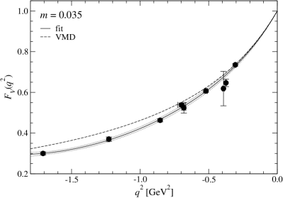
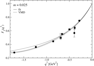
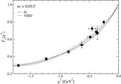
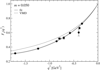
The vector form factor FV(q2)subscript𝐹𝑉superscript𝑞2F_{V}(q^{2}) is plotted as a function of q2superscript𝑞2q^{2} in Fig. 12. Its q2superscript𝑞2q^{2} dependence turns out to be close to the expectation from the vector meson dominance (VMD) hypothesis

FV(q2)subscript𝐹𝑉superscript𝑞2\displaystyle F_{V}(q^{2}) =\displaystyle= 11q2/Mρ2,11superscript𝑞2superscriptsubscript𝑀𝜌2\displaystyle\frac{1}{1-q^{2}/M_{\rho}^{2}}, (34)

where Mρsubscript𝑀𝜌M_{\rho} is the vector meson mass calculated at the same quark mass. Then, we assume that the small deviation due to higher poles or cuts can be well parametrized by a polynomial form. We therefore fit our data to the following form

FV(q2)subscript𝐹𝑉superscript𝑞2\displaystyle F_{V}(q^{2}) =\displaystyle= 11q2/Mρ2+aV,1q2+aV,2(q2)2+aV,3(q2)311superscript𝑞2superscriptsubscript𝑀𝜌2subscript𝑎𝑉1superscript𝑞2subscript𝑎𝑉2superscriptsuperscript𝑞22subscript𝑎𝑉3superscriptsuperscript𝑞23\displaystyle\frac{1}{1-q^{2}/M_{\rho}^{2}}+a_{V,1}\,q^{2}+a_{V,2}\,(q^{2})^{2}+a_{V,3}\,(q^{2})^{3} (35)

in order to extract the charge radius r2Vsubscriptdelimited-⟨⟩superscript𝑟2𝑉\langle r^{2}\rangle_{V} and the curvature cVsubscript𝑐𝑉c_{V}

r2V=6FV(q2)(q2)|q2=0,cV=2FV(q2)(q2)2|q2=0.formulae-sequencesubscriptdelimited-⟨⟩superscript𝑟2𝑉evaluated-at6subscript𝐹𝑉superscript𝑞2superscript𝑞2superscript𝑞20subscript𝑐𝑉evaluated-atsuperscript2subscript𝐹𝑉superscript𝑞2superscriptsuperscript𝑞22superscript𝑞20\displaystyle\langle r^{2}\rangle_{V}=\left.6\frac{\partial F_{V}(q^{2})}{\partial(q^{2})}\right|_{q^{2}=0},\hskip 28.45274ptc_{V}=\left.\frac{\partial^{2}F_{V}(q^{2})}{\partial(q^{2})^{2}}\right|_{q^{2}=0}. (36)

The fit curve is plotted in Fig. 12 and numerical results are summarized in Table 9. The fit describes our data reasonably well, and results for r2Vsubscriptdelimited-⟨⟩superscript𝑟2𝑉\langle r^{2}\rangle_{V} and cVsubscript𝑐𝑉c_{V} do not change significantly by including or excluding the cubic term aV,3(q2)3subscript𝑎𝑉3superscriptsuperscript𝑞23a_{V,3}(q^{2})^{3}. In the following analysis, we employ results from the parametrization with the cubic term.
Refer to caption
Refer to caption
Refer to caption
Refer to caption
Figure 12: Vector form factor FV(q2)subscript𝐹𝑉superscript𝑞2F_{V}(q^{2}) as a function of q2superscript𝑞2q^{2}. Solid and dotted lines show the fit curve (35) and its error. The q2superscript𝑞2q^{2} dependence from the vector meson dominance model is shown by the dashed line.
Table 9: Parametrization Eq. (35) for vector form factor FV(q2)subscript𝐹𝑉superscript𝑞2F_{V}(q^{2}). Results for the vector radius r2Vsubscriptdelimited-⟨⟩superscript𝑟2𝑉\langle r^{2}\rangle_{V} and curvature cVsubscript𝑐𝑉c_{V} in lattice units are also listed.
m𝑚m χ2/d.o.f.formulae-sequencesuperscript𝜒2dof\chi^{2}/{\rm d.o.f.} aV,1subscript𝑎𝑉1a_{V,1} aV,2subscript𝑎𝑉2a_{V,2} aV,3subscript𝑎𝑉3a_{V,3} r2Vsubscriptdelimited-⟨⟩superscript𝑟2𝑉\langle r^{2}\rangle_{V} cVsubscript𝑐𝑉c_{V}
0.050 1.8(0.8) 0.187(33) 0.181(55) 18.72(20) 8.786(55)
0.050 1.7(0.9) 0.116(64) -0.22(26) -0.48(28) 18.30(38) 8.38(26)
0.035 1.3(0.5) 0.136(60) 0.124(96) 20.15(36) 10.51(10)
0.035 1.2(0.7) 0.02(11) -0.50(44) -0.73(46) 19.48(66) 9.88(44)
0.025 1.9(0.6) 0.034(90) -0.03(14) 21.69(54) 12.78(14)
0.025 1.7(0.7) -0.14(16) -0.98(59) -1.10(56) 20.64(98) 11.83(59)
0.015 0.8(0.8) -0.09(12) -0.15(19) 22.51(72) 14.58(19)
0.015 0.5(0.8) -0.35(25) -1.56(96) -1.60(95) 20.9(1.5) 13.18(96)
Refer to caption
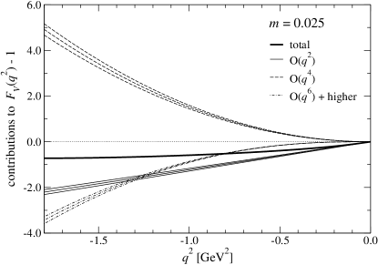
Figure 13: Contributions in the q2superscript𝑞2q^{2} expansion of FV(q2)1subscript𝐹𝑉superscript𝑞21F_{V}(q^{2})\!-\!1 at m=0.025𝑚0.025m\!=\!0.025. Thin solid, dashed and dot-dashed lines show O(q2)𝑂superscript𝑞2O(q^{2}), O(q4)𝑂superscript𝑞4O(q^{4}) and higher contributions, whereas the thick solid line is their total.

One of the main purposes of this work is to investigate whether the q2superscript𝑞2q^{2} dependence of our data can be described by two-loop ChPT PFF_V:ChPT:NNLO:2 ; PFF_V:ChPT:NNLO . Figure 13 shows contributions to FV(q2)subscript𝐹𝑉superscript𝑞2F_{V}(q^{2}) from each order (q2)nsuperscriptsuperscript𝑞2𝑛(q^{2})^{n} of a Taylor expansion of Eq. (35). We find that O(q6)𝑂superscript𝑞6O(q^{6}) and higher order contributions to FV(q2)subscript𝐹𝑉superscript𝑞2F_{V}(q^{2}) are sufficiently small only below |q2|0.3GeV2similar-to-or-equalssuperscript𝑞20.3superscriptGeV2|q^{2}|\!\simeq\!0.3~{}\mbox{GeV}^{2}, which is however around our smallest value of |q2|superscript𝑞2|q^{2}|. We therefore do not use the parametrization based on ChPT in this study. Note that such large higher order contributions are unavoidable unless |q2|Mρ2much-less-thansuperscript𝑞2superscriptsubscript𝑀𝜌2|q^{2}|\!\ll\!M_{\rho}^{2}, because the VMD form is a good approximation of FV(q2)subscript𝐹𝑉superscript𝑞2F_{V}(q^{2}).

Table 10: Single pole fit (37). We also list the ρ𝜌\rho meson mass at simulated quark masses.
m𝑚m χ2/d.o.f.formulae-sequencesuperscript𝜒2dof\chi^{2}/{\rm d.o.f.} Mpolesubscript𝑀poleM_{\rm pole} r2Vsubscriptdelimited-⟨⟩superscript𝑟2𝑉\langle r^{2}\rangle_{V} cVsubscript𝑐𝑉c_{V} Mρsubscript𝑀𝜌M_{\rho}
0.050 4.3(1.1) 0.5431(50) 20.34(38) 11.49(43) 0.5839(28)
0.035 2.3(0.7) 0.5270(80) 21.61(65) 12.97(78) 0.5570(31)
0.025 2.9(0.8) 0.511(11) 23.0(1.0) 14.6(1.3) 0.5285(43)
0.015 0.7(0.7) 0.520(16) 22.2(1.4) 13.7(1.7) 0.5104(55)

We also test a single pole ansatz often used in the previous studies

FV(q2)subscript𝐹𝑉superscript𝑞2\displaystyle F_{V}(q^{2}) =\displaystyle= 11q2/Mpole2.11superscript𝑞2superscriptsubscript𝑀pole2\displaystyle\frac{1}{1-q^{2}/M_{\rm pole}^{2}}. (37)

As summarized in Table 10, this fit tends to give a slightly higher χ2superscript𝜒2\chi^{2} and r2Vsubscriptdelimited-⟨⟩superscript𝑟2𝑉\langle r^{2}\rangle_{V} than those from Eq. (35). This may suggest that it is difficult to describe our precise data of FV(q2)subscript𝐹𝑉superscript𝑞2F_{V}(q^{2}) in the whole region of q2[GeV2][1.7,0]superscript𝑞2delimited-[]superscriptGeV21.70q^{2}[\mbox{GeV}^{2}]\!\in\![-1.7,0] by a simple pole-dominance form.

IV.2 Scalar form factor

Refer to caption
Refer to caption
Refer to caption
Refer to caption
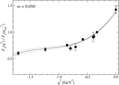
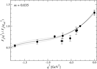
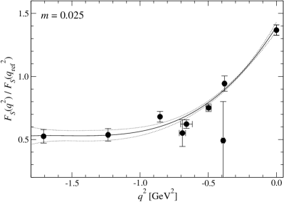
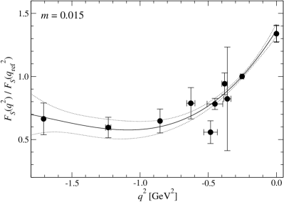
Figure 14: Normalized scalar form factor FS(q2)/FS(qref2)subscript𝐹𝑆superscript𝑞2subscript𝐹𝑆superscriptsubscript𝑞ref2F_{S}(q^{2})/F_{S}(q_{\rm ref}^{2}) as a function of q2superscript𝑞2q^{2}. Solid and dotted lines show the cubic fit and its error.
Table 11: Parametrization Eq. (38) for scalar form factor FS(q2)subscript𝐹𝑆superscript𝑞2F_{S}(q^{2}). Results for the vector radius r2Ssubscriptdelimited-⟨⟩superscript𝑟2𝑆\langle r^{2}\rangle_{S} and curvature cSsubscript𝑐𝑆c_{S} in lattice units are also listed.
m𝑚m χ2/d.o.f.formulae-sequencesuperscript𝜒2dof\chi^{2}/{\rm d.o.f.} aS,1subscript𝑎𝑆1a_{S,1} aS,2subscript𝑎𝑆2a_{S,2} aS,3subscript𝑎𝑆3a_{S,3} aS,4subscript𝑎𝑆4a_{S,4} r2Ssubscriptdelimited-⟨⟩superscript𝑟2𝑆\langle r^{2}\rangle_{S} cSsubscript𝑐𝑆c_{S}
0.050 1.3(1.0) 3.04(31) 6.6(1.3) 5.1(1.4) 18.2(1.9) 6.6(1.3)
0.050 1.3(1.1) 3.51(49) 10.5(3.5) 1.6(9.2) 9.6(7.7) 21.1(3.0) 10.5(3.5)
0.035 1.8(1.0) 2.79(31) 5.6(1.4) 4.3(1.6) 16.8(1.9) 5.6(1.4)
0.035 1.9(1.2) 2.60(51) 3.5(4.8) -3(15) -6(13) 15.6(3.1) 3.5(4.8)
0.025 1.9(1.1) 3.37(32) 6.1(1.6) 3.6(1.8) 20.2(1.9) 6.1(1.6)
0.025 1.9(1.3) 2.97(53) 1.8(4.6) -9(13) -12(11) 17.8(3.2) 1.8(4.6)
0.015 1.5(1.0) 3.51(51) 6.6(2.7) 3.6(3.3) 21.0(3.1) 6.6(2.7)
0.015 1.7(1.1) 3.0(1.0) 1.0(9.1) -14(26) -16(22) 18.1(6.0) 1.0(9.1)

Due to the lack of knowledge about the scalar resonances at the simulated quark masses, we test a generic polynomial form up to the quartic order

FS(q2)subscript𝐹𝑆superscript𝑞2\displaystyle F_{S}(q^{2}) =\displaystyle= FS(0){1+aS,1q2+aS,2(q2)2+aS,3(q2)3+aS,4(q2)4}subscript𝐹𝑆01subscript𝑎𝑆1superscript𝑞2subscript𝑎𝑆2superscriptsuperscript𝑞22subscript𝑎𝑆3superscriptsuperscript𝑞23subscript𝑎𝑆4superscriptsuperscript𝑞24\displaystyle F_{S}(0)\left\{1+a_{S,1}\,q^{2}+a_{S,2}\,(q^{2})^{2}+a_{S,3}\,(q^{2})^{3}+a_{S,4}\,(q^{2})^{4}\right\} (38)

to parametrize the q2superscript𝑞2q^{2} dependence of the scalar form factor FS(q2)subscript𝐹𝑆superscript𝑞2F_{S}(q^{2}). We observe that the cubic (aS,4=0subscript𝑎𝑆40a_{S,4}\!=\!0) fit also describes our data reasonably well as seen in Fig. 14. Fit results summarized in Table 11 show that the inclusion of the quartic correction does not change the value of χ2superscript𝜒2\chi^{2} and the result for the scalar radius r2S=6aS,1subscriptdelimited-⟨⟩superscript𝑟2𝑆6subscript𝑎𝑆1\langle r^{2}\rangle_{S}\!=\!6\,a_{S,1} significantly. However, such a stability against the choice of the parametrization is much less clear in the curvature cS=aS,2subscript𝑐𝑆subscript𝑎𝑆2c_{S}\!=\!a_{S,2} due to its large uncertainty. From these observations, we only use results for r2Ssubscriptdelimited-⟨⟩superscript𝑟2𝑆\langle r^{2}\rangle_{S} in the following analysis, and leave a precise determination of cSsubscript𝑐𝑆c_{S} for future studies.

V Chiral extrapolation

V.1 Fit based on one-loop ChPT

Since the form factors FV,S(q2)subscript𝐹𝑉𝑆superscript𝑞2F_{V,S}(q^{2}) are independent of q2superscript𝑞2q^{2} at LO in ChPT, the chiral expansion of the radii r2V,Ssubscriptdelimited-⟨⟩superscript𝑟2𝑉𝑆\langle r^{2}\rangle_{V,S} starts from the one-loop order of ChPT. We first compare our lattice results with the one-loop expressions PFF:ChPT:NLO:1

r2Vsubscriptdelimited-⟨⟩superscript𝑟2𝑉\displaystyle\langle r^{2}\rangle_{V} =\displaystyle= 1NF2(1+6Nl6r)1NF2ln[Mπ2μ2],1𝑁superscript𝐹216𝑁superscriptsubscript𝑙6𝑟1𝑁superscript𝐹2superscriptsubscript𝑀𝜋2superscript𝜇2\displaystyle-\frac{1}{NF^{2}}\left(1+6N\,l_{6}^{r}\right)-\frac{1}{NF^{2}}\ln\left[\frac{M_{\pi}^{2}}{\mu^{2}}\right], (39)
r2Ssubscriptdelimited-⟨⟩superscript𝑟2𝑆\displaystyle\langle r^{2}\rangle_{S} =\displaystyle= 1NF2(132+6Nl4r)6NF2ln[Mπ2μ2],1𝑁superscript𝐹21326𝑁superscriptsubscript𝑙4𝑟6𝑁superscript𝐹2superscriptsubscript𝑀𝜋2superscript𝜇2\displaystyle\frac{1}{NF^{2}}\left(-\frac{13}{2}+6N\,l_{4}^{r}\right)-\frac{6}{NF^{2}}\ln\left[\frac{M_{\pi}^{2}}{\mu^{2}}\right], (40)

where N=(4π)2𝑁superscript4𝜋2N\!=\!(4\pi)^{2}, and F𝐹F is the decay constant in the chiral limit. We adopt the normalization of the decay constant Fπ=92subscript𝐹𝜋92F_{\pi}\!=\!92 MeV at the physical quark mass. The renormalization scale μ𝜇\mu is set to 4πF4𝜋𝐹4\pi F in our analysis. At this order of the chiral expansion, F𝐹F is the only LEC appearing in the Mπsubscript𝑀𝜋M_{\pi} dependent terms. We fix this important parameter to F=79.0(2.6+5.0)F\!=\!79.0(^{+5.0}_{-2.6}) MeV, which has been determined from our detailed analysis of the pion mass and decay constant Spectrum:Nf2:RG+Ovr:JLQCD . Each one of Eqs. (39) and (40), therefore, has a single fit parameter, namely LECs l6rsuperscriptsubscript𝑙6𝑟l_{6}^{r} or l4rsuperscriptsubscript𝑙4𝑟l_{4}^{r} in their constant term.

Refer to caption
Refer to caption
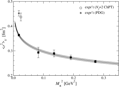
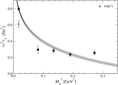
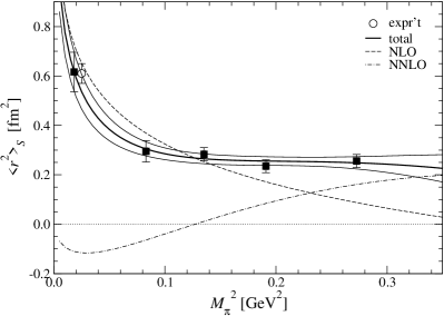
Figure 15: Chiral fit of r2Vsubscriptdelimited-⟨⟩superscript𝑟2𝑉\langle r^{2}\rangle_{V} (left panel) and r2Ssubscriptdelimited-⟨⟩superscript𝑟2𝑆\langle r^{2}\rangle_{S} (right panel) using one-loop ChPT formulae. Filled squares are the lattice data and the value extrapolated to the physical point. In the left panel, we also plot the experimental value r2V=0.437(16)fm2subscriptdelimited-⟨⟩superscript𝑟2𝑉0.43716superscriptfm2\langle r^{2}\rangle_{V}\!=\!0.437(16)~{}\mbox{fm}^{2} from an analysis based on Nf=2subscript𝑁𝑓2N_{f}\!=\!2 ChPT PFF_V:ChPT:NNLO (open circle) and 0.452(11)fm20.45211superscriptfm20.452(11)~{}\mbox{fm}^{2} quoted by Particle Data Group PDG:2008 (star). The star symbol in the right panel represents r2S=0.61(4)fm2subscriptdelimited-⟨⟩superscript𝑟2𝑆0.614superscriptfm2\langle r^{2}\rangle_{S}\!=\!0.61(4)~{}\mbox{fm}^{2} obtained from an indirect determination through ππ𝜋𝜋\pi\pi scattering PFF_S:ChPT:NNLO .

We find that the NLO fits of lattice data are not quite successful as seen in Fig. 15 and Table 12. While the data of r2Vsubscriptdelimited-⟨⟩superscript𝑟2𝑉\langle r^{2}\rangle_{V} can be fitted with reasonable χ2/d.o.f.0.14\chi^{2}/{\rm d.o.f.}\!\sim\!0.14, the value extrapolated to the physical quark mass r2V=0.3637(43)fm2subscriptdelimited-⟨⟩superscript𝑟2𝑉0.363743superscriptfm2\langle r^{2}\rangle_{V}\!=\!0.3637(43)~{}\mbox{fm}^{2} is significantly smaller than the experimental value 0.437(16)fm20.43716superscriptfm20.437(16)~{}\mbox{fm}^{2} based on Nf=2subscript𝑁𝑓2N_{f}\!=\!2 ChPT PFF_V:ChPT:NNLO and 0.452(11)fm20.45211superscriptfm20.452(11)~{}\mbox{fm}^{2} quoted by PDG PDG:2008 . As for the scalar radius, the one-loop formula fails to reproduce our data of r2Ssubscriptdelimited-⟨⟩superscript𝑟2𝑆\langle r^{2}\rangle_{S} as indicated by the quite large value of χ2/d.o.f.9\chi^{2}/{\rm d.o.f.}\!\sim\!9 : the data have a mild quark mass dependence in contrast to the 666 times enhanced chiral logarithm compared to r2Vsubscriptdelimited-⟨⟩superscript𝑟2𝑉\langle r^{2}\rangle_{V}.

Table 12: Results of chiral extrapolations of r2Vsubscriptdelimited-⟨⟩superscript𝑟2𝑉\langle r^{2}\rangle_{V} and r2Ssubscriptdelimited-⟨⟩superscript𝑟2𝑆\langle r^{2}\rangle_{S} using one-loop ChPT formulae Eqs. (39) and (40). The radii extrapolated to the physical point are also listed.
χ2/d.o.f.formulae-sequencesuperscript𝜒2dof\chi^{2}/{\rm d.o.f.} l6r×103superscriptsubscript𝑙6𝑟superscript103l_{6}^{r}\times 10^{3} r2V[fm2]subscriptdelimited-⟨⟩superscript𝑟2𝑉delimited-[]superscriptfm2\langle r^{2}\rangle_{V}[\mbox{fm}^{2}] χ2/d.o.f.formulae-sequencesuperscript𝜒2dof\chi^{2}/{\rm d.o.f.} l4r×103superscriptsubscript𝑙4𝑟superscript103l_{4}^{r}\times 10^{3} r2S[fm2]subscriptdelimited-⟨⟩superscript𝑟2𝑆delimited-[]superscriptfm2\langle r^{2}\rangle_{S}[\mbox{fm}^{2}]
0.14 -6.59(12) 0.3637(43) 9.0 2.94(39) 0.797(15)

This failure of the NLO fits is not due to our choice of F𝐹F. If F𝐹F is treated as a free parameter, the fit to r2Ssubscriptdelimited-⟨⟩superscript𝑟2𝑆\langle r^{2}\rangle_{S} results in an unacceptably large value F200similar-to-or-equals𝐹200F\!\simeq\!200 MeV to achieve reasonable χ2/d.o.f.1\chi^{2}/{\rm d.o.f.}\lesssim 1, whereas our data of r2Vsubscriptdelimited-⟨⟩superscript𝑟2𝑉\langle r^{2}\rangle_{V} favor F80similar-to𝐹80F\!\sim\!80 MeV. Thus we can not make a consistent analysis. We note that we have experienced a similar situation, namely r2Vsubscriptdelimited-⟨⟩superscript𝑟2𝑉\langle r^{2}\rangle_{V} smaller than experiment and a small quark mass dependence of r2Ssubscriptdelimited-⟨⟩superscript𝑟2𝑆\langle r^{2}\rangle_{S}, in our previous study with a different lattice action PFF:Nf2:Plq+Clv:JLQCD , though simulated quark masses are heavier than those in this study.

We also note that the lattice data for the curvature cVsubscript𝑐𝑉c_{V} largely deviate from its NLO ChPT expression as shown below. From all of these observations we conclude that the chiral behavior of the pion form factors in the quark mass region ms/6subscript𝑚𝑠6m_{s}/6 – ms/2subscript𝑚𝑠2m_{s}/2 are not well described by NLO ChPT.

V.2 Fit based on two-loop ChPT

In Ref. Spectrum:Nf2:RG+Ovr:JLQCD , we observed that NNLO contributions are important to reliably extract LECs from the pion mass and decay constant in our simulated region of the quark mass. Therefore there exists a possibility that NNLO contributions become also important to describe the chiral behaviour of the radii. The two-loop expressions of r2V,Ssubscriptdelimited-⟨⟩superscript𝑟2𝑉𝑆\langle r^{2}\rangle_{V,S} and cVsubscript𝑐𝑉c_{V} are given by PFF_V:ChPT:NNLO ; PFF_V:ChPT:NNLO:2

r2Vsubscriptdelimited-⟨⟩superscript𝑟2𝑉\displaystyle\langle r^{2}\rangle_{V} =\displaystyle= 1NF2(1+6Nl6r)1NF2ln[Mπ2μ2]1𝑁superscript𝐹216𝑁superscriptsubscript𝑙6𝑟1𝑁superscript𝐹2superscriptsubscript𝑀𝜋2superscript𝜇2\displaystyle-\frac{1}{NF^{2}}\left(1+6N\,l_{6}^{r}\right)-\frac{1}{NF^{2}}\ln\left[\frac{M_{\pi}^{2}}{\mu^{2}}\right] (41)
+1N2F4(13N19218148+6N2rV,rr)Mπ2+1N2F4(19612Nl1,2r)Mπ2ln[Mπ2μ2],1superscript𝑁2superscript𝐹413𝑁192181486superscript𝑁2superscriptsubscript𝑟𝑉𝑟𝑟superscriptsubscript𝑀𝜋21superscript𝑁2superscript𝐹419612𝑁superscriptsubscript𝑙12𝑟superscriptsubscript𝑀𝜋2superscriptsubscript𝑀𝜋2superscript𝜇2\displaystyle+\frac{1}{N^{2}F^{4}}\left(\frac{13N}{192}-\frac{181}{48}+6N^{2}r_{V,r}^{r}\right)\,M_{\pi}^{2}+\frac{1}{N^{2}F^{4}}\left(\frac{19}{6}-12Nl_{1,2}^{r}\right)M_{\pi}^{2}\ln\left[\frac{M_{\pi}^{2}}{\mu^{2}}\right],\hskip 14.22636pt
r2Ssubscriptdelimited-⟨⟩superscript𝑟2𝑆\displaystyle\langle r^{2}\rangle_{S} =\displaystyle= 1NF2(132+6Nl4r)6NF2ln[Mπ2μ2]1𝑁superscript𝐹21326𝑁superscriptsubscript𝑙4𝑟6𝑁superscript𝐹2superscriptsubscript𝑀𝜋2superscript𝜇2\displaystyle\frac{1}{NF^{2}}\left(-\frac{13}{2}+6N\,l_{4}^{r}\right)-\frac{6}{NF^{2}}\ln\left[\frac{M_{\pi}^{2}}{\mu^{2}}\right] (42)
+1N2F4(23N192+869108+88Nl1,2r+80Nl2r+5Nl3r24N2l3rl4r+6N2rS,rr)Mπ21superscript𝑁2superscript𝐹423𝑁19286910888𝑁superscriptsubscript𝑙12𝑟80𝑁superscriptsubscript𝑙2𝑟5𝑁superscriptsubscript𝑙3𝑟24superscript𝑁2superscriptsubscript𝑙3𝑟superscriptsubscript𝑙4𝑟6superscript𝑁2superscriptsubscript𝑟𝑆𝑟𝑟superscriptsubscript𝑀𝜋2\displaystyle+\frac{1}{N^{2}F^{4}}\left(-\frac{23N}{192}+\frac{869}{108}+88Nl_{1,2}^{r}+80Nl_{2}^{r}+5Nl_{3}^{r}-24N^{2}l_{3}^{r}l_{4}^{r}+6N^{2}r_{S,r}^{r}\right)\,M_{\pi}^{2}
+1N2F4(32336+124Nl1,2r+130Nl2r)Mπ2ln[Mπ2μ2]653N2F4Mπ2ln[Mπ2μ2]2,\displaystyle+\frac{1}{N^{2}F^{4}}\left(-\frac{323}{36}+124Nl_{1,2}^{r}+130Nl_{2}^{r}\right)\,M_{\pi}^{2}\ln\left[\frac{M_{\pi}^{2}}{\mu^{2}}\right]-\frac{65}{3N^{2}F^{4}}M_{\pi}^{2}\ln\left[\frac{M_{\pi}^{2}}{\mu^{2}}\right]^{2},\hskip 14.22636pt
cVsubscript𝑐𝑉\displaystyle c_{V} =\displaystyle= 160NF21Mπ2+1N2F4(N720842925920+N3l1,2r+N6l6r+N2rV,cr)160𝑁superscript𝐹21superscriptsubscript𝑀𝜋21superscript𝑁2superscript𝐹4𝑁720842925920𝑁3superscriptsubscript𝑙12𝑟𝑁6superscriptsubscript𝑙6𝑟superscript𝑁2superscriptsubscript𝑟𝑉𝑐𝑟\displaystyle\frac{1}{60NF^{2}}\frac{1}{M_{\pi}^{2}}+\frac{1}{N^{2}F^{4}}\left(\frac{N}{720}-\frac{8429}{25920}+\frac{N}{3}l_{1,2}^{r}+\frac{N}{6}l_{6}^{r}+N^{2}r_{V,c}^{r}\right) (43)
+1N2F4(1108+N3l1,2r+N6l6r)ln[Mπ2μ2]+172N2F4ln[Mπ2μ2]2,\displaystyle+\frac{1}{N^{2}F^{4}}\left(\frac{1}{108}+\frac{N}{3}l_{1,2}^{r}+\frac{N}{6}l_{6}^{r}\right)\,\ln\left[\frac{M_{\pi}^{2}}{\mu^{2}}\right]+\frac{1}{72N^{2}F^{4}}\ln\left[\frac{M_{\pi}^{2}}{\mu^{2}}\right]^{2},

where we use a linear combination l1,2r=l1rl2r/2superscriptsubscript𝑙12𝑟superscriptsubscript𝑙1𝑟superscriptsubscript𝑙2𝑟2l_{1,2}^{r}=l_{1}^{r}-l_{2}^{r}/2 instead of l1rsuperscriptsubscript𝑙1𝑟l_{1}^{r}, since the former is convenient for our chiral extrapolation (see below). The analytic terms containing r{V,S},{r,c}rsuperscriptsubscript𝑟𝑉𝑆𝑟𝑐𝑟r_{\{V,S\},\{r,c\}}^{r} represent contributions of tree diagrams with vertices from the O(p6)𝑂superscript𝑝6O(p^{6}) chiral Lagrangian.

Table 13: Phenomenological estimates of LECs used in this paper. We note that O(p6)𝑂superscript𝑝6O(p^{6}) couplings r{V,S},{r,c}rsuperscriptsubscript𝑟𝑉𝑆𝑟𝑐𝑟r_{\{V,S\},\{r,c\}}^{r} are based on a resonance saturation hypothesis.
Ref.F:ChPT:NNLO Ref.PFF_S:ChPT:NNLO Ref.PFF:ChPT:NLO:1 Ref.PFF_V:ChPT:NNLO
F𝐹F[MeV] l¯1subscript¯𝑙1\bar{l}_{1} l¯2subscript¯𝑙2\bar{l}_{2} l¯4subscript¯𝑙4\bar{l}_{4} l¯3subscript¯𝑙3\bar{l}_{3} l¯6subscript¯𝑙6\bar{l}_{6} rV,rr×104superscriptsubscript𝑟𝑉𝑟𝑟superscript104r_{V,r}^{r}\times 10^{4} rV,cr×104superscriptsubscript𝑟𝑉𝑐𝑟superscript104r_{V,c}^{r}\times 10^{4} rS,rr×104superscriptsubscript𝑟𝑆𝑟𝑟superscript104r_{S,r}^{r}\times 10^{4}
86.2(5) -0.36(59) 4.31(11) 4.39(22) 2.9(2.4) 16.0(9) -2.5 2.6 -0.3
Refer to caption
Refer to caption
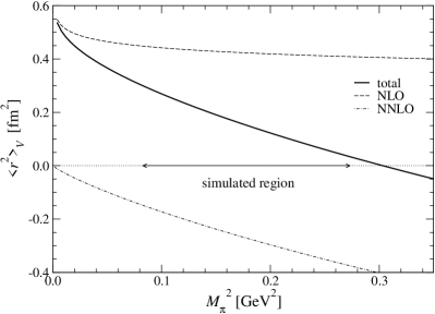
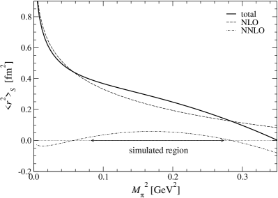
Figure 16: Chiral behavior of radii based on two-loop ChPT with phenomenological estimates of LECs listed in Table 13. The dashed and dot-dashed lines represent contributions at NLO and NNLO, whereas the solid line is their total. We note that r{V,S},{r,c}rsuperscriptsubscript𝑟𝑉𝑆𝑟𝑐𝑟r_{\{V,S\},\{r,c\}}^{r} from the resonance saturation are taken as the renormalized LECs at the resonance mass scale in this plot.

Before fitting lattice data to these expressions, one can get some idea about the significance of the NNLO contributions by using phenomenological estimates of LECs. A collection of recent estimates is shown in Table 13, where the LECs in the O(p4)𝑂superscript𝑝4O(p^{4}) chiral Lagrangian are denoted by the scale invariant convention l¯isubscript¯𝑙𝑖\bar{l}_{i} defined by

lir=γi2N(l¯i+ln[Mπ2μ2])superscriptsubscript𝑙𝑖𝑟subscript𝛾𝑖2𝑁subscript¯𝑙𝑖superscriptsubscript𝑀𝜋2superscript𝜇2\displaystyle l_{i}^{r}=\frac{\gamma_{i}}{2N}\left(\bar{l}_{i}+\ln\left[\frac{M_{\pi}^{2}}{\mu^{2}}\right]\right) (44)

with

γ1=13,γ2=23,γ3=12,γ4=2,γ6=13.formulae-sequencesubscript𝛾113formulae-sequencesubscript𝛾223formulae-sequencesubscript𝛾312formulae-sequencesubscript𝛾42subscript𝛾613\displaystyle\gamma_{1}=\frac{1}{3},\hskip 5.69054pt\gamma_{2}=\frac{2}{3},\hskip 5.69054pt\gamma_{3}=-\frac{1}{2},\hskip 5.69054pt\gamma_{4}=2,\hskip 5.69054pt\gamma_{6}=-\frac{1}{3}. (45)

Figure 16 shows the expected Mπ2superscriptsubscript𝑀𝜋2M_{\pi}^{2} dependence of r2Vsubscriptdelimited-⟨⟩superscript𝑟2𝑉\langle r^{2}\rangle_{V} and r2Ssubscriptdelimited-⟨⟩superscript𝑟2𝑆\langle r^{2}\rangle_{S} from Eqs. (41) and (42) with the phenomenological estimates of LECs. The individual contributions from NLO and NNLO are also plotted. This analysis suggests that the NNLO contributions could significantly modify the chiral behavior of the radii in our simulated quark masses. However, we note that r{V,S},{r,c}rsuperscriptsubscript𝑟𝑉𝑆𝑟𝑐𝑟r_{\{V,S\},\{r,c\}}^{r} are poorly known and these in Table 13 are determined from a resonance saturation hypothesis. A chiral extrapolation of lattice data with the two-loop formulae is therefore important to confirm the significance of the NNLO contributions and to resolve the failure of the one-loop fit.

The curvature cVsubscript𝑐𝑉c_{V} characterizes the O(q4)𝑂superscript𝑞4O(q^{4}) dependence of FV(q2)subscript𝐹𝑉superscript𝑞2F_{V}(q^{2}), and therefore requires the NNLO terms to describe its logarithmic dependence on the quark mass as well as a constant term. Near the chiral limit it has a divergent term of the form 1/(F2Mπ2)similar-toabsent1superscript𝐹2superscriptsubscript𝑀𝜋2\sim 1/(F^{2}M_{\pi}^{2}), which comes from non-analytic NLO contributions in FV(q2)subscript𝐹𝑉superscript𝑞2F_{V}(q^{2}). Since the divergent term 1/(F2Mπ2)1superscript𝐹2superscriptsubscript𝑀𝜋21/(F^{2}M_{\pi}^{2}) is significant only below the physical pion mass, the analysis of the lattice data for cVsubscript𝑐𝑉c_{V} requires the NNLO contributions.

We extend our analysis to two-loop ChPT as already outlined in our previous report Lat08:JLQCD:TK . The curvature cVsubscript𝑐𝑉c_{V} is included into our chiral extrapolation to obtain an additional constraint on LECs. Both of r2Vsubscriptdelimited-⟨⟩superscript𝑟2𝑉\langle r^{2}\rangle_{V} and cVsubscript𝑐𝑉c_{V} depend on l1rsuperscriptsubscript𝑙1𝑟l_{1}^{r} and l2rsuperscriptsubscript𝑙2𝑟l_{2}^{r} only through the linear combination l1,2rsuperscriptsubscript𝑙12𝑟l_{1,2}^{r}, and the complicated two-loop expressions for r2Vsubscriptdelimited-⟨⟩superscript𝑟2𝑉\langle r^{2}\rangle_{V} and cVsubscript𝑐𝑉c_{V} involve only four free parameters l6rsuperscriptsubscript𝑙6𝑟l_{6}^{r}, l1,2rsuperscriptsubscript𝑙12𝑟l_{1,2}^{r}, rV,rrsuperscriptsubscript𝑟𝑉𝑟𝑟r_{V,r}^{r} and rV,crsuperscriptsubscript𝑟𝑉𝑐𝑟r_{V,c}^{r} by choosing Mπ2/(4πF)2superscriptsubscript𝑀𝜋2superscript4𝜋𝐹2M_{\pi}^{2}/(4\pi F)^{2} as an expansion parameter. Therefore we first try a simultaneous fit to r2Vsubscriptdelimited-⟨⟩superscript𝑟2𝑉\langle r^{2}\rangle_{V} and cVsubscript𝑐𝑉c_{V} to check that the chiral behavior of our data is described by two-loop ChPT. Fit curves are plotted in Fig. 17 and numerical results are summarized in Table 14. The fit leads to an acceptable value of χ2/d.o.f.0.7\chi^{2}/{\rm d.o.f.}\sim 0.7, and the relevant LECs are determined with a reasonable accuracy. We note that this fit is based only on ChPT without additional assumptions. The extrapolated values of r2Vsubscriptdelimited-⟨⟩superscript𝑟2𝑉\langle r^{2}\rangle_{V} and cVsubscript𝑐𝑉c_{V} are consistent with recent phenomenological determinations using experimental data of FV(q2)subscript𝐹𝑉superscript𝑞2F_{V}(q^{2}) PFF_V:ChPT:NNLO ; cV:DR:AR ; cV:ChPT_DR:GHLM ; r2+cV:Pade:MPS .
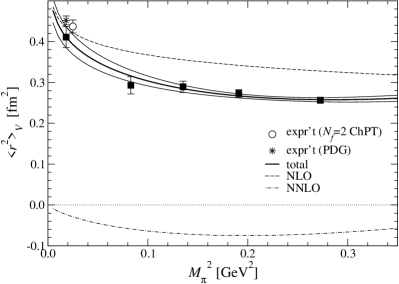
Refer to caption
Refer to caption
Figure 17: Simultaneous chiral fit to r2Vsubscriptdelimited-⟨⟩superscript𝑟2𝑉\langle r^{2}\rangle_{V} and cVsubscript𝑐𝑉c_{V} based on two-loop formulae Eqs. (41) and (43). The experimental value for cV=3.85(0.60)subscript𝑐𝑉3.850.60c_{V}\!=\!3.85(0.60) is taken from Ref. PFF_V:ChPT:NNLO .
Table 14: Results of simultaneous chiral fit to r2Vsubscriptdelimited-⟨⟩superscript𝑟2𝑉\langle r^{2}\rangle_{V} and cVsubscript𝑐𝑉c_{V} based on two-loop formulae Eqs. (41) and (43).
χ2/d.o.f.formulae-sequencesuperscript𝜒2dof\chi^{2}/{\rm d.o.f.} l6r×103superscriptsubscript𝑙6𝑟superscript103l_{6}^{r}\times 10^{3} l12r×103superscriptsubscript𝑙12𝑟superscript103{l}_{12}^{r}\times 10^{3} rV,rr×105superscriptsubscript𝑟𝑉𝑟𝑟superscript105r_{V,r}^{r}\times 10^{5} rV,cr×105superscriptsubscript𝑟𝑉𝑐𝑟superscript105r_{V,c}^{r}\times 10^{5} r2V[fm2]subscriptdelimited-⟨⟩superscript𝑟2𝑉delimited-[]superscriptfm2\langle r^{2}\rangle_{V}[\mbox{fm}^{2}] cV[GeV4]subscript𝑐𝑉delimited-[]superscriptGeV4c_{V}[\mbox{GeV}^{-4}]
0.70 -8.48(87) -3.3(1.1) -0.77(69) 3.97(20) 0.411(26) 3.26(21)

In Sec. IV, we observe that the O(q6)𝑂superscript𝑞6O(q^{6}) contribution to FV(q2)subscript𝐹𝑉superscript𝑞2F_{V}(q^{2}) is not small in the simulated region of the momentum transfer q20.3GeV2greater-than-or-equivalent-tosuperscript𝑞20.3superscriptGeV2q^{2}\gtrsim 0.3~{}\mbox{GeV}^{2} (q2/(4πF)20.3greater-than-or-equivalent-tosuperscript𝑞2superscript4𝜋𝐹20.3q^{2}/(4\pi F)^{2}\gtrsim 0.3). The q2superscript𝑞2q^{2} dependence of our data is therefore parametrized by the generic polynomial forms (35) and (38) instead of those based on ChPT. This is not in contradiction with the successful chiral extrapolation of r2Vsubscriptdelimited-⟨⟩superscript𝑟2𝑉\langle r^{2}\rangle_{V} and cVsubscript𝑐𝑉c_{V}: since we explore small pion masses Mπ20.3GeV2less-than-or-similar-tosuperscriptsubscript𝑀𝜋20.3superscriptGeV2M_{\pi}^{2}\lesssim 0.3~{}\mbox{GeV}^{2} (Mπ2/(4πF)20.3less-than-or-similar-tosuperscriptsubscript𝑀𝜋2superscript4𝜋𝐹20.3M_{\pi}^{2}/(4\pi F)^{2}\lesssim 0.3), the quark mass dependence of r2Vsubscriptdelimited-⟨⟩superscript𝑟2𝑉\langle r^{2}\rangle_{V} and cVsubscript𝑐𝑉c_{V} is described by the two-loop ChPT formulae.

The inclusion of r2Ssubscriptdelimited-⟨⟩superscript𝑟2𝑆\langle r^{2}\rangle_{S} into the simultaneous chiral fit introduces additional four free parameters l2rsuperscriptsubscript𝑙2𝑟l_{2}^{r}, l3rsuperscriptsubscript𝑙3𝑟l_{3}^{r}, l4rsuperscriptsubscript𝑙4𝑟l_{4}^{r} and rS,rrsuperscriptsubscript𝑟𝑆𝑟𝑟r_{S,r}^{r}, and we need to fix some of them to obtain a stable fit. Since l2rsuperscriptsubscript𝑙2𝑟l_{2}^{r} and l3rsuperscriptsubscript𝑙3𝑟l_{3}^{r} appear only in the NNLO terms and have been determined with a reasonable accuracy from phenomenology or lattice studies, we use a phenomenological estimate l¯2=4.31(11)subscript¯𝑙24.3111\bar{l}_{2}\!=\!4.31(11) PFF_S:ChPT:NNLO and a lattice estimate l¯3=3.38(56)subscript¯𝑙33.3856\bar{l}_{3}\!=\!3.38(56) from our analysis of the pion spectroscopy Spectrum:Nf2:RG+Ovr:JLQCD . We treat rS,rrsuperscriptsubscript𝑟𝑆𝑟𝑟r_{S,r}^{r} and l4rsuperscriptsubscript𝑙4𝑟l_{4}^{r} as free parameters because of poor knowledge on the former and in order to examine the consistency of the latter with that determined from Fπsubscript𝐹𝜋F_{\pi}. The fit curves are shown in Fig. 18 and numerical results are summarized in Table 15. We observe that i) the results in the vector channel, namely r2Vsubscriptdelimited-⟨⟩superscript𝑟2𝑉\langle r^{2}\rangle_{V}, cVsubscript𝑐𝑉c_{V} and the relevant LECs, do not change significantly by including r2Ssubscriptdelimited-⟨⟩superscript𝑟2𝑆\langle r^{2}\rangle_{S} into the chiral fit, and ii) this fit describes the mild quark mass dependence of r2Ssubscriptdelimited-⟨⟩superscript𝑟2𝑆\langle r^{2}\rangle_{S} with an acceptable value of χ2/d.o.f.0.7\chi^{2}/{\rm d.o.f.}\!\sim\!0.7. From Fig. 18, we find that the net NNLO contribution to r2Ssubscriptdelimited-⟨⟩superscript𝑟2𝑆\langle r^{2}\rangle_{S} is larger than NLO around our largest quark mass. This is due to an accidental cancellation between the constant and logarithmic terms at NLO.
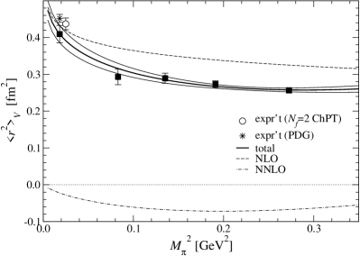
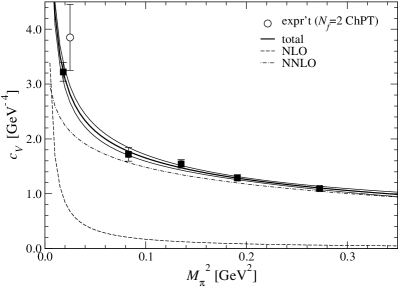
Refer to caption
Refer to caption
Refer to caption
Figure 18: Simultaneous chiral fit for radii r2V,Ssubscriptdelimited-⟨⟩superscript𝑟2𝑉𝑆\langle r^{2}\rangle_{V,S} and curvature cVsubscript𝑐𝑉c_{V}.
Table 15: Results of simultaneous chiral fit to r2V,Ssubscriptdelimited-⟨⟩superscript𝑟2𝑉𝑆\langle r^{2}\rangle_{V,S} and cVsubscript𝑐𝑉c_{V} based on two-loop formulae Eqs. (41), (42) and (43).
χ2/d.o.f.formulae-sequencesuperscript𝜒2dof\chi^{2}/{\rm d.o.f.} l6r×103superscriptsubscript𝑙6𝑟superscript103l_{6}^{r}\times 10^{3} l4r×103superscriptsubscript𝑙4𝑟superscript103l_{4}^{r}\times 10^{3} l1,2r×103superscriptsubscript𝑙12𝑟superscript103l_{1,2}^{r}\times 10^{3} rV,rr×105superscriptsubscript𝑟𝑉𝑟𝑟superscript105r_{V,r}^{r}\times 10^{5} rV,cr×105superscriptsubscript𝑟𝑉𝑐𝑟superscript105r_{V,c}^{r}\times 10^{5} rS,rr×104superscriptsubscript𝑟𝑆𝑟𝑟superscript104r_{S,r}^{r}\times 10^{4} r2V[fm2]subscriptdelimited-⟨⟩superscript𝑟2𝑉delimited-[]superscriptfm2\langle r^{2}\rangle_{V}[\mbox{fm}^{2}] cV[GeV4]subscript𝑐𝑉delimited-[]superscriptGeV4c_{V}[\mbox{GeV}^{-4}] r2S[fm2]subscriptdelimited-⟨⟩superscript𝑟2𝑆delimited-[]superscriptfm2\langle r^{2}\rangle_{S}[\mbox{fm}^{2}]
0.68 -8.41(76) 1.1(3.2) -3.10(90) -1.0(1.1) 4.00(17) 1.74(36) 0.409(23) 3.22(17) 0.617(79)

We take results from this simultaneous fit as our best estimate of r2V,Ssubscriptdelimited-⟨⟩superscript𝑟2𝑉𝑆\langle r^{2}\rangle_{V,S}, cVsubscript𝑐𝑉c_{V}. The systematic error due to the chiral extrapolation is estimated by excluding the data at the largest quark mass from the fit. The shifts in the radii and curvature turn out to be at the 1 σ𝜎\sigma level: namely, the extrapolation is stable against variation of the fit range. In order to estimate systematics due to the fixed topology and the use of the Feynman-Hellmann theorem to estimate FS(0)subscript𝐹𝑆0F_{S}(0), we repeat the whole analysis by using FV,S(q2)subscript𝐹𝑉𝑆superscript𝑞2F_{V,S}(q^{2}) shifted by their systematic uncertainties discussed in Secs. III.2 and III.4. Systematic uncertainties due to the choice of the inputs, namely LECs F𝐹F, l2rsuperscriptsubscript𝑙2𝑟l_{2}^{r}, l3rsuperscriptsubscript𝑙3𝑟l_{3}^{r} for the chiral extrapolation and r0=0.49subscript𝑟00.49r_{0}\!=\!0.49 fm to fix the scale, are estimated by shifting each LEC by its uncertainty and by using a recent lattice estimate r0=0.47subscript𝑟00.47r_{0}\!=\!0.47 fm r0:Nf2:ImpG+Asqt:MILC:1 ; r0:Nf2:ImpG+Asqt:MILC:2 . In addition, a discretization error estimated by a naive order counting O((aΛQCD)2)3𝑂superscript𝑎subscriptΛQCD23O((a\Lambda_{\rm QCD})^{2})\approx 3 % is also taken into account. The magnitude of these systematic uncertainties are summarized in Table 16. Our final results for the radii and curvature at the physical point are

r2Vsubscriptdelimited-⟨⟩superscript𝑟2𝑉\displaystyle\langle r^{2}\rangle_{V} =\displaystyle= 0.409(23)(37)fm2,0.4092337superscriptfm2\displaystyle 0.409(23)(37)~{}\mbox{fm}^{2}, (46)
r2Ssubscriptdelimited-⟨⟩superscript𝑟2𝑆\displaystyle\langle r^{2}\rangle_{S} =\displaystyle= 0.617(79)(66)fm2,0.6177966superscriptfm2\displaystyle 0.617(79)(66)~{}\mbox{fm}^{2}, (47)
cVsubscript𝑐𝑉\displaystyle c_{V} =\displaystyle= 3.22(17)(36)GeV4,3.221736superscriptGeV4\displaystyle 3.22(17)(36)~{}\mbox{GeV}^{-4}, (48)

where the first error is statistical and the second represents systematic errors added in quadrature. These results are in good agreement with their phenomenological values. The largest systematic error arises from the use of the input r0subscript𝑟0r_{0} to fix the scale. This can be removed by a better choice, such as fπsubscript𝑓𝜋f_{\pi}, in future studies in three-flavor QCD.

Table 16: Statistical and systematic errors of radii and curvature. We list the magnitude of the errors relative to the central values.
stat. sys.(total) chiral fit input(LECs) input(r0subscript𝑟0r_{0}) fixed Q𝑄Q Feynman-Hellmann finite a𝑎a
r2Vsubscriptdelimited-⟨⟩superscript𝑟2𝑉\langle r^{2}\rangle_{V} 6 % 9 % 5.3 % 0.2 % 6.1 % 2.2 % 1.4 % 3.0 %
r2Ssubscriptdelimited-⟨⟩superscript𝑟2𝑆\langle r^{2}\rangle_{S} 13% 11% 4.0 % 2.2 % 7.7 % 2.4 % 4.6 % 3.0 %
cVsubscript𝑐𝑉c_{V} 5 % 11 % 2.7 % 0.4 % 9.3 % 2.3 % 3.8 % 3.0 %

We estimate the relevant LECs in a similar way to that for r2V,Ssubscriptdelimited-⟨⟩superscript𝑟2𝑉𝑆\langle r^{2}\rangle_{V,S} and cVsubscript𝑐𝑉c_{V}, and obtain

l¯6subscript¯𝑙6\displaystyle\bar{l}_{6} =\displaystyle= 11.9(0.7)(1.0),11.90.71.0\displaystyle 11.9(0.7)(1.0), (49)
l¯4subscript¯𝑙4\displaystyle\bar{l}_{4} =\displaystyle= 4.09(50)(52),4.095052\displaystyle 4.09(50)(52), (50)
l¯1l¯2subscript¯𝑙1subscript¯𝑙2\displaystyle\bar{l}_{1}-\bar{l}_{2} =\displaystyle= 2.9(0.9)(1.3),2.90.91.3\displaystyle-2.9(0.9)(1.3), (51)
rV,rrsuperscriptsubscript𝑟𝑉𝑟𝑟\displaystyle r_{V,r}^{r} =\displaystyle= 1.0(1.0)(2.5)×105,1.01.02.5superscript105\displaystyle-1.0(1.0)(2.5)\times 10^{-5}, (52)
rV,crsuperscriptsubscript𝑟𝑉𝑐𝑟\displaystyle r_{V,c}^{r} =\displaystyle= 4.00(17)(64)×105,4.001764superscript105\displaystyle 4.00(17)(64)\times 10^{-5}, (53)
rS,rrsuperscriptsubscript𝑟𝑆𝑟𝑟\displaystyle r_{S,r}^{r} =\displaystyle= 1.74(36)(78)×104.1.743678superscript104\displaystyle 1.74(36)(78)\times 10^{-4}. (54)

Our estimate of l¯6subscript¯𝑙6\bar{l}_{6} is slightly smaller than those from two-loop ChPT analyses of experimental data; l¯6=16.0(0.9)subscript¯𝑙616.00.9\bar{l}_{6}\!=\!16.0(0.9) from FVsubscript𝐹𝑉F_{V} PFF_V:ChPT:NNLO and 15.2(0.4) from τ𝜏\tau and π𝜋\pi decays l6:ChPT:NNLO:tau+pi . This is partly due to the deviation of F𝐹F between our lattice determination Spectrum:Nf2:RG+Ovr:JLQCD and two-loop ChPT F:ChPT:NNLO . We note that l¯4subscript¯𝑙4\bar{l}_{4} is consistent with our lattice determination l¯4=4.12(56)subscript¯𝑙44.1256\bar{l}_{4}\!=\!4.12(56) from Fπsubscript𝐹𝜋F_{\pi} Spectrum:Nf2:RG+Ovr:JLQCD and a phenomenological estimate 4.39(22) PFF_S:ChPT:NNLO . Here we list l¯1l¯2subscript¯𝑙1subscript¯𝑙2\bar{l}_{1}\!-\!\bar{l}_{2} instead of l1,2rsuperscriptsubscript𝑙12𝑟l_{1,2}^{r}, which is scale invariant and equals to (l¯1l¯2)/(6N)subscript¯𝑙1subscript¯𝑙26𝑁(\bar{l}_{1}\!-\!\bar{l}_{2})/(6N) in the convention of Eq. (44). Although l¯1l¯2subscript¯𝑙1subscript¯𝑙2\bar{l}_{1}\!-\!\bar{l}_{2} has a large uncertainty of similar-to\sim 50 %, it is consistent with 4.67(60)4.6760-4.67(60) from phenomenology. Note that we set the renormalization scale μ=4πF𝜇4𝜋𝐹\mu\!=\!4\pi F, and our fit favors small values of the order of 104superscript10410^{-4} – 105superscript10510^{-5} for the renormalized O(p6)𝑂superscript𝑝6O(p^{6}) couplings r{V,S},{r,c}rsubscriptsuperscript𝑟𝑟𝑉𝑆𝑟𝑐r^{r}_{\{V,S\},\{r,c\}} at this scale. Finally, we emphasize that the simultaneous fit only to r2Vsubscriptdelimited-⟨⟩superscript𝑟2𝑉\langle r^{2}\rangle_{V} and cVsubscript𝑐𝑉c_{V} without any phenomenological input leads to consistent results for the vector channel, namely for r2Vsubscriptdelimited-⟨⟩superscript𝑟2𝑉\langle r^{2}\rangle_{V}, cVsubscript𝑐𝑉c_{V}, l¯6subscript¯𝑙6\bar{l}_{6}, l¯1l¯2subscript¯𝑙1subscript¯𝑙2\bar{l}_{1}\!-\!\bar{l}_{2} and rV,{r,c}rsuperscriptsubscript𝑟𝑉𝑟𝑐𝑟r_{V,\{r,c\}}^{r}.

VI Conclusions

In this article, we present a lattice calculation of the pion form factors FV,S(q2)subscript𝐹𝑉𝑆superscript𝑞2F_{V,S}(q^{2}) in two-flavor QCD. We study the chiral behavior of the radii r2V,Ssubscriptdelimited-⟨⟩superscript𝑟2𝑉𝑆\langle r^{2}\rangle_{V,S} and the curvature cVsubscript𝑐𝑉c_{V} based on ChPT up to two loops. We employ the overlap quark action, which has exact chiral symmetry and thus provides the cleanest framework for the study of chiral behavior. Otherwise, the explicit chiral symmetry breaking of conventional lattice actions could make studies based on two-loop ChPT substantially complicated. Another salient feature of this work is that, for the first time, FS(q2)subscript𝐹𝑆superscript𝑞2F_{S}(q^{2}) is evaluated including the contributions of the disconnected diagrams through the all-to-all quark propagators.

Our detailed analysis based on ChPT reveals that two-loop contributions are important to describe the chiral behavior of r2V,Ssubscriptdelimited-⟨⟩superscript𝑟2𝑉𝑆\langle r^{2}\rangle_{V,S} and cVsubscript𝑐𝑉c_{V} at our simulated quark masses, which are comparable to those in recent unquenched simulations. Through the chiral extrapolation at two loops, we obtain r2V,Ssubscriptdelimited-⟨⟩superscript𝑟2𝑉𝑆\langle r^{2}\rangle_{V,S} and cVsubscript𝑐𝑉c_{V} at the physical point, which are consistent with experiment. We also obtain estimates of O(p4)𝑂superscript𝑝4O(p^{4}) and O(p6)𝑂superscript𝑝6O(p^{6}) LECs, and confirm that FS(q2)subscript𝐹𝑆superscript𝑞2F_{S}(q^{2}) and Fπsubscript𝐹𝜋F_{\pi} lead to consistent results for l¯4subscript¯𝑙4\bar{l}_{4} as suggested long ago PFF:ChPT:NLO:1 .

As we already outlined in Ref. Lat08:JLQCD:TK , the curvature cVsubscript𝑐𝑉c_{V} is useful to stabilize the two-loop chiral fit. The single pole ansatz Eq. (37), which has been commonly used in previous studies, may not be suitable to estimate cVsubscript𝑐𝑉c_{V}, since it simply assumes a relation cV=(r2V/6)2subscript𝑐𝑉superscriptsubscriptdelimited-⟨⟩superscript𝑟2𝑉62c_{V}\!=\!(\langle r^{2}\rangle_{V}/6)^{2} at simulated quark masses. In this work, instead, we employ a generic form up to cubic corrections to parametrize the q2superscript𝑞2q^{2} dependence of FV,S(q2)subscript𝐹𝑉𝑆superscript𝑞2F_{V,S}(q^{2}) thanks to the precise determination of FV,S(q2)subscript𝐹𝑉𝑆superscript𝑞2F_{V,S}(q^{2}) through the all-to-all propagator. Dispersive analyses of the q2superscript𝑞2q^{2} dependence, model independent information of scalar resonances, and the twisted boundary condition TBC already used in Refs.PFF:Nf3:RG+DW:RBC+UKQCD ; PFF:Nf2:Sym+tmW:ETMC are interesting subject and technique for a better control of this parametrization in future studies.

Extending this study to three-flavor QCD is important for more realistic comparison with experiment. We have already started simulations in three-flavor QCD with the overlap action Lat07:JLQCD:Matsufuru ; Lat08:JLQCD:Hashimoto ; measurements of pion correlators using all-to-all propagators are in progress.

Finally, it is expected from our chiral extrapolation that r2Ssubscriptdelimited-⟨⟩superscript𝑟2𝑆\langle r^{2}\rangle_{S} shows a strong quark mass dependence due to the one-loop chiral logarithm below Mπ250similar-tosubscript𝑀𝜋250M_{\pi}\!\sim\!250 MeV. Pushing simulations toward such small quark masses is an interesting subject in future studies for a direct observation of the one-loop logarithm, although it is very challenging.

Acknowledgements.
Numerical simulations are performed on Hitachi SR11000 and IBM System Blue Gene Solution at High Energy Accelerator Research Organization (KEK) under a support of its Large Scale Simulation Program (No. 08-05). This work is supported in part by the Grant-in-Aid of the Ministry of Education (No. 18340075, 18740167, 19540286, 19740160, 20025010, 20039005, 20105001, 20105002, 20105003, 20105005, 20340047, 20740156 and 21684013), the National Science Council of Taiwan (No. NSC96-2112-M-002-020-MY3, NSC96-2112-M-001-017-MY3, NSC97-2119-M-002-001), and NTU-CQSE (No. 97R0066-65 and 97R0066-69).

References

  • (1) H. Matsufuru, PoS LATTICE 2007, 018 (2007) [arXiv:0710.4225 [hep-lat]].
  • (2) S. Hashimoto, PoS LATTICE 2008, 011 (2008) [arXiv:0811.1257 [hep-lat]].
  • (3) R. Narayanan and H. Neuberger, Nucl. Phys. B443, 305 (1995) [arXiv:hep-th/9411108].
  • (4) H. Neuberger, Phys. Lett. B 417, 141 (1998) [arXiv:hep-lat/9707022]; ibid. B 427, 353 (1998) [arXiv:hep-lat/9801031].
  • (5) J. Noaki et al. (JLQCD and TWQCD collaborations), Phys. Rev. Lett. 101, 202004 (2008) [arXiv:0806.0894 [hep-lat]].
  • (6) H. Fukaya et al. (JLQCD collaboration), Phys. Rev. Lett. 98, 172001 (2007) [arXiv:hep-lat/0702003].
  • (7) H. Fukaya et al. (JLQCD and TWQCD collaborations), Phys. Rev. D76, 054503 (2007) [arXiv:0705.3322 [hep-lat]].
  • (8) S. Aoki et al. (JLQCD and TWQCD collaborations), Phys. Lett. B 665, 294 (2008) [arXiv:0710.1130 [hep-lat]].
  • (9) H. Fukaya et al. (JLQCD collaboration), Phys. Rev. D77, 074503 (2008) [arXiv:0711.4965 [hep-lat]].
  • (10) S. Aoki et al. (JLQCD collaboration), Phys. Rev. D 77, 094503 (2008) [arXiv:arXiv:0801.4186 [hep-lat]].
  • (11) E. Shintani et al. (JLQCD collaboration), Phys. Rev. Lett. 101, 242001 (2008) [arXiv:0806.4222 [hep-lat]].
  • (12) H. Ohki et al. (JLQCD collaboration), Phys. Rev. D 78, 054502 (2008) [arXiv:0806.4744 [hep-lat]].
  • (13) E. Shintani et al. (JLQCD and TWQCD collaborations), arXiv:0807.0556 [hep-lat].
  • (14) J. Gasser and H. Leutwyler, Ann. Phys. 158, 142 (1984).
  • (15) J. Gasser and U.-G. Meißner, Nucl. Phys. B 357, 90 (1991).
  • (16) J. Bijnens, G. Colangelo and P. Talavera, JHEP 9805, 014 (1998) [arXiv:hep-ph/9805389].
  • (17) J. Gasser and H. Leutwyler, Nucl. Phys. B 250, 517 (1985).
  • (18) J. Bijnens and P. Talavera, JHEP 0203, 046 (2002) [arXiv:hep-ph/0203049].
  • (19) Y. Nemoto (RBC collaboration), Nucl. Phys. B (Proc.Suppl.) 129, 299 (2004), [arXiv:hep-lat/0309173].
  • (20) J. van der Heide, J.H. Koch and E. Laermann, Phys. Rev. D 69, 094511 (2004) [arXiv:hep-lat/0312023].
  • (21) A.M. Abdel-Rehim and R. Lewis, Phys. Rev. D 71, 014503 (2005), [arXiv:hep-lat/0410047].
  • (22) F.D.R. Bonnet, R.G. Edwards, G.T. Fleming, R. Lewis, D.G. Richards (LHP collaboration), Phys. Rev. D 72, 054506 (2005) [arXiv:hep-lat/0411028].
  • (23) S. Hashimoto et al. (JLQCD collaboration), PoS LAT2005, 336 (2005) [arXiv:hep-lat/0510085].
  • (24) D. Brömmel et al. (QCDSF and UKQCD collaborations), Eur. Phys. J. C 51, 335 (2007) [arXiv:hep-lat/0608021].
  • (25) S. Capitani, C. Gattringer and C.B. Lang (BGR collaboration), Phys. Rev. D 73, 034505 (2006) [arXiv:hep-lat/0511040].
  • (26) P.A. Boyle et al. (RBC and UKQCD collaborations), JHEP 0807, 112 (2008) [arXiv:0804.3971 [hep-lat]].
  • (27) R. Frezzotti, V. Lubicz, S. Simula (ETM collaboration), arXiv:0812.4042 [hep-lat].
  • (28) T. Kaneko et al. (JLQCD and TWQCD collaborations), PoS LATTICE 2008 158, (2008) [arXiv:0810.2590 [hep-lat]].
  • (29) T. Kaneko et al. (JLQCD collaboration), PoS LATTICE 2007, 148 (2007) [arXiv:0710.2390 [hep-lat]].
  • (30) Y. Iwasaki, preprint UTHEP-118 (1983), unpublished.
  • (31) M. Lüscher, Phys. Lett. B 428, 342 (1998) [arXiv:hep-lat/9802011].
  • (32) N. Yamada et al. (JLQCD collaboration), PoS LAT2006, 060 (2006) [arXiv:hep-lat/0609073].
  • (33) S. Aoki et al. (JLQCD collaboration), Phys. Rev. D 78, 014508 (2008) [arXiv:0803.3197 [hep-lat]].
  • (34) Z. Fodor, S. D. Katz and K. K. Szabo, JHEP 0408, 003 (2004) [arXiv:hep-lat/0311010].
  • (35) P. M. Vranas, arXiv:hep-lat/0001006; Phys. Rev. D 74, 034512 (2006) [arXiv:hep-lat/0606014].
  • (36) H. Fukaya et al. (JLQCD collaboration), Phys. Rev. D 74, 094505 (2006) [arXiv:hep-lat/0607020].
  • (37) R. Brower, S. Chandrasekharan, J. W. Negele and U.-J. Wiese, Phys. Lett. B 560, 64 (2003) [arXiv:hep-lat/0302005].
  • (38) S. Aoki, H. Fukaya, S. Hashimoto and T. Onogi, Phys. Rev. D 76, 054508 (2007) [arXiv:0707.0396 [hep-lat]].
  • (39) R. Sommer, Nucl. Phys. B 411, 839 (1994) [arXiv:hep-lat/9310022].
  • (40) J. Foley et al. (TrinLat collaboration), Comput. Phys. Commun, 172, 145 (2005) [arXiv:hep-lat/0505023].
  • (41) N. Cundy et al., Comput. Phys. Commun. 165, 221 (2005) [arXiv:hep-lat/0405003].
  • (42) L. Giusti, P. Hernandez, M. Laine, P. Weisz and H. Wittig, JHEP 0404, 013 (2004) [arXiv:hep-lat/0402002].
  • (43) T.A. DeGrand, S. Schaefer, Comput. Phys. Commun. 159, 185 (2004) [arXiv:hep-lat/0401011].
  • (44) S. Hashimoto et al., Phys. Rev. D 61, 014502 (1999) [arXiv:hep-ph/9906376].
  • (45) T.B. Bunton, F.-J. Jiang and B.C. Tiburzi, Phys. Rev. D 74, 034514 (2006) [arXiv:hep-lat/0607001, Erratum-ibid. D 74, 099902 (2006)].
  • (46) B. Borasoy and R. Lewis, Phys. Rev. D 71, 014033 (2005) [arXiv:hep-lat/0410042].
  • (47) D. Bećirević and G. Villadoro, Phys. Rev. D 69, 054010 (2004) [arXiv:hep-lat/0311028].
  • (48) C.T. Sachrajda and G. Villadoro, Phys. Lett. B 609, 73 (2005) [arXiv:hep-lat/0411033].
  • (49) C. Amsler et al. (Particle Data Group), Phys. Lett. B 667, 1 (2008).
  • (50) G. Colangelo, J. Gasser and H. Leutwyler, Nucl. Phys. B 603, 125 (2001) [arXiv:hep-ph/0103088].
  • (51) G. Colangelo and S. Dürr, Eur. Phys. J. C 33, 543 (2004) [arXiv:hep-lat/0311023].
  • (52) B. Ananthanarayan and S. Ramanan, arXiv:0811.0482 [hep-ph].
  • (53) F.-K. Guo, C. Hanhart, F.J. Llanes-Estrada and U.-G. Meißner, arXiv:0812.3270 [hep-ph].
  • (54) P. Masjuan, S. Peris and J.J. Sanz-Cillero, Phys. Rev. D 78, 074028 (2008) [arXiv:0807.4893 [hep-ph]].
  • (55) A. Bazavov et al. (MILC collaboration), arXiv:0903.3598 [hep-lat].
  • (56) C. Aubin et al. (MILC collaboration), Phys. Rev. D 70, 094505 (2004) [arXiv:hep-lat/0402030].
  • (57) M. Gonzárez-Alonso, A. Pich and J. Prades, Phys. Rev. D 78, 116012 (2008) [arXiv:0810.0760 [hep-ph]].
  • (58) P.F. Bedaque, Phys. Lett. B 593, 82 (2004) [arXiv:nucl-th/0402051].