Generalized Kernel-based Visual Tracking

Abstract

Kernel-based mean shift (MS) trackers have proven to be a promising alternative to stochastic particle filtering trackers. Despite its popularity, MS trackers have two fundamental drawbacks: (1) The template model can only be built from a single image; (2) It is difficult to adaptively update the template model. In this work we generalize the plain MS trackers and attempt to overcome these two limitations.

It is well known that modeling and maintaining a representation of a target object is an important component of a successful visual tracker. However, little work has been done on building a robust template model for kernel-based MS tracking. In contrast to building a template from a single frame, we train a robust object representation model from a large amount of data. Tracking is viewed as a binary classification problem, and a discriminative classification rule is learned to distinguish between the object and background. We adopt a support vector machine (SVM) for training. The tracker is then implemented by maximizing the classification score. An iterative optimization scheme very similar to MS is derived for this purpose. Compared with the plain MS tracker, it is now much easier to incorporate on-line template adaptation to cope with inherent changes during the course of tracking. To this end, a sophisticated on-line support vector machine is used. We demonstrate successful localization and tracking on various data sets.

I Introduction

Visual localization/tracking plays a central role for many applications like intelligent video surveillance, smart transportation monitoring systems etc. Localization and tracking algorithms aim to find the most similar region to the target in an image. Recently, kernel-based tracking algorithms [1, 2, 3] have attracted much attention as an alternative to particle filtering trackers [4, 5, 6]. One of the most crucial difficulties in robust tracking is the construction of representation models (likelihood models in Bayesian filtering trackers) that can accommodate illumination variations, deformable appearance changes, partial occlusions, etc. Most current tracking algorithms use a single static template image to construct a target representation based on density models. For both kernel-based trackers and particle filtering trackers, a popular method is to exploit color distributions in simple regions (region-wise density models). Generally semi-parametric kernel density estimation techniques are adopted. However, it is difficult to update this target model [1, 2, 4, 7], and the target representation’s fragility usually breaks these trackers over a long image sequence.

Considerable effort has been expended to ease these difficulties. We believe that the key to finding a solution is to find the right representation. In order to accommodate appearance changes, the representation model should be learned from as many training examples as possible. Fundamentally two methods, namely on-line and off-line learning, can be used for the training procedure. On-line learning means constantly updating the representation model during the course of tracking. [8] proposes an incremental eigenvector update strategy to adapt the target representation model. A linear probabilistic principal component analysis model is used. The main disadvantage of the eigen-model is that it is not generic and is usually only suitable for characterizing texture-rich objects. In [9] a wavelet model is updated using the expectation maximization (EM) algorithm. A classification function is progressively learned using AdaBoost for visual detection and tracking in [10] and [11] respectively. [12] adopts pixel-wise Gaussian mixture models (GMMs) to represent the target model and sequentially update them. To date, however, less work has been reported on how to elegantly update region-wise density models in tracking.

In contrast, classification is a powerful bottom-up procedure: It is trained off-line and works on-line. Due to the training being typically built on very large amounts of training data, its performance is fairly promising even without on-line updating of the classifier/detector. Inspired by image classification tasks with color density features and real-time detection, we learn off-line a density representation model from multiple training data. By considering tracking as a binary classification problem, a discriminative classification rule is learned to distinguish between the tracked object and background patterns. In this way a robust object representation model is obtained. This proposal provides a basis for considering the design of enhanced kernel-based trackers using robust kernel object representations. A by-product of the training is the classification function, with which the tracking problem is cast into a binary classification problem. An object detector directly using the classification function is then available. Combining a detector into the tracker makes the tracker more robust and provides the capabilities of automatic initialization and recovery from momentary tracking failures.

In theory, many classifiers can be used to achieve our goal. In this paper we show that the popular kernel based non-linear support vector machine (SVM) well fits the kernel-based tracking framework. Within this framework the traditional kernel object trackers proposed in [1] and [13] can be expressed as special cases. Because we use probabilistic density features, the learning process is closely related to probabilistic kernels based SVMs [14, 15, 16, 17]. It is imperative to minimize computational costs for real-time applications such as tracking. A desirable property of the proposed algorithm is that the computational complexity is independent of the number of support vectors. Furthermore we empirically demonstrate that our algorithm requires fewer iterations to achieve convergence.

Our approach differs from [18] although both use the SVM classification score as the cost function. In [18], Avidan builds a tracker along the line of standard optical flow tracking. Only the homogeneous quadratic polynomial kernel (or kernels with a similar quadratic structure) can be used in order to derive a closed-form solution. This restriction prevents one using a more appropriate kernel obtained by model selection. An advantage of [18] is that it can be used consistently with the optical flow tracking, albeit only gray pixel information can be used. Moreover, the optimization procedure of our approach is inspired by the kernel-based object tracking paradigm [1]. Hence extended work such as [2] is also applicable here, which enables us to find the global optimum. If joint spatial-feature density is used to train an SVM, a fixed-point optimization method may also be derived that is similar to [13]. The classification function of the SVM trained for vehicle recognition is not smooth w.r.t. spatial mis-registration (see Fig. 1 in [19]). We employ a spatial kernel to smooth the cost function when computing the histogram feature. In this way, gradient based optimization methods can be used. Using statistical learning theory, we devise an object tracker that is consistent with MS tracking. The MS tracker is initially derived from kernel density estimation (KDE). Our work sheds some light on the connection between SVM and KDE.

Another important part of our tracker is its on-line re-training in parallel with tracking. Continuous updating of the representation model can capture changes of the target appearance/backgrounds. Previous work such as [9, 11, 8, 12] has demonstrated the importance of this on-line update during the course of tracking. The incremental SVM technique meets this end [22, 23, 24, 25], which efficiently updates a trained SVM function whenever a sample is added to or removed from the training set. For our proposed tracking framework, the target model can be learned in either batch SVM training or on-line SVM learning. We adopt a sophisticated on-line SVM learning proposed in [24] for its efficiency and simplicity. We address the crucial problem of adaptation, i.e., the on-line learning of discriminant appearance model while avoiding drift.

The main contributions of our work are to solve MS trackers’ two drawbacks: The template model can only be built from a single image; and it is difficult to update the model. The solution is to extend the use of statistical learning algorithms for object localization and tracking. SVM has been used for tracking by means of spatial perturbation of the SVM [18]. We exploit SVM for tracking in a novel way (along the line of MS tracking). The key ingredients of our approach are:

• Probabilistic kernel based SVMs are trained and incorporated into the framework of MS tracking. By carefully selecting the kernel, we show that no extra computation is required compared with the conventional single-view MS tracking.

• An on-line SVM can be used to adaptively update the target model. We demonstrate the benefit of on-line target model update.

• We show that the annealed MS algorithm proposed in [2] can be viewed as a special case of the continuation method under an appropriate interpretation. With the new interpretation, annealed MS can be extended to more general cases. Extension and new discovers are discussed. An efficient localizer is built with global mode seeking techniques.

• Again, by exploiting the SVM binary classifier, it is able to determine the scale of the target. An improved annealed MS-like algorithm with a cascade architecture is developed. It enables a more systematic and easier design of the annealing schedule, in contrast with ad hoc methods in previous work [2].

The remainder of the paper is organized as follows. In §II, the general theory of MS tracking and SVM is reviewed for completeness. Our proposed tracker is presented in §III. Finally experimental results are reported in §IV. We conclude this work in §V.

II Preliminaries

For self-completeness, we review mean shift tracking, support vector machine and its on-line learning version in this section.

II-A Mean Shift Tracking

Mean shift (MS) tracking was firstly presented in [1]. In MS tracking, the object is represented by a square region which is cropped and normalized into a unit circle. By denoting ${\mathbf{q}}$ as the color histogram of the target model, and ${\mathbf{p}}({\mathbf{c}})$ as the target candidate color histogram with the center at ${\mathbf{c}}$, the similarity function between ${\mathbf{q}}$ and ${\mathbf{p}}({\mathbf{c}})$ is (when Bhattacharyya divergence [1] is used),

$${{\rm dist}}({\mathbf{q}},{\mathbf{p}}({\mathbf{c}}))=\sqrt{1-\varrho({\mathbf{q}},{\mathbf{p}})}.$$

Here $\varrho({\mathbf{q}},{\mathbf{p}})=\sqrt{{\mathbf{q}}}^{\!\top}\sqrt{{\mathbf{p}}}$ is the dissimilarity measurement. Let $\{{\mathbf{I}}_{\ell}\}_{\ell=1}^{n}$ be a region’s pixel positions in image ${\mathbf{I}}$ with the center at ${\mathbf{c}}$. In order to make the cost function smooth—otherwise gradient based MS optimization cannot be applied—a kernel with profile $k(\cdot)$ is employed to assign smaller weights to those pixels farther from the center, considering the fact that the peripheral pixels are less reliable. An $m$-bin color histogram is built for an image patch located at ${\mathbf{c}}$, ${\mathbf{q}}({\mathbf{c}})=\{q_{u}({\mathbf{c}})\}_{u=1}^{m}$, where

$$q_{u}=\lambda\sum_{\ell=1}^{n}k\Bigl{(}\Bigl{\|}\frac{{\mathbf{c}}-{\mathbf{I}}_{\ell}}{h}\Bigr{\|}^{2}\Bigr{)}\delta(\vartheta({\mathbf{I}}_{\ell})-u).$$ (1)

Here $k(\cdot)$ is the homogeneous spatial weighting kernel profile and $h$ is its bandwidth. $\delta(\cdot)$ is the delta function and $\lambda$ normalizes ${\mathbf{q}}$. The function $\vartheta({\mathbf{I}}_{\ell})$ maps a feature of ${\mathbf{I}}_{\ell}$ into a histogram bin $u$. ${\mathbf{c}}$ is the kernel center; and for the target model usually ${\mathbf{c}}=0$. The representation of candidate ${\mathbf{p}}$ takes the same form.

Given an initial position ${\mathbf{c}}_{0}$, the problem of localization/tracking is to estimate a best displacement $\Delta{\mathbf{c}}$ such that the measurement ${\mathbf{p}}({\mathbf{c}}_{0}+\Delta{\mathbf{c}})$ at the new location best matches the target ${\mathbf{q}}$, i.e.,

$$\Delta{\mathbf{c}}^{\star}=\mathop{\mathrm{argmin}}\limits\nolimits_{\Delta{\mathbf{c}}}{{{\rm dist}}({\mathbf{q}},{\mathbf{p}}({\mathbf{c}}_{0}+\Delta{\mathbf{c}}))}.$$

By Taylor expanding ${{\rm dist}}({\mathbf{q}},{\mathbf{p}}({\mathbf{c}}))$ at the start position ${\mathbf{c}}_{0}$ and keeping only the linear item (first-order Taylor approximation), the above optimization problem can be resolved by an iterative procedure:

$${\mathbf{c}}^{[\tau+1]}=\frac{\sum_{\ell=1}^{n}{{\mathbf{I}}_{\ell}{\widetilde{w}}_{\ell}g(\|\frac{{\mathbf{c}}^{[\tau]}-{\mathbf{I}}_{\ell}}{h}\|^{2})}}{\sum_{\ell=1}^{n}{{\widetilde{w}}_{\ell}g(\|\frac{{\mathbf{c}}^{[\tau]}-{\mathbf{I}}_{\ell}}{h}\|^{2})}},$$ (2)

where $g(\cdot)=-k^{\prime}(\cdot)$ and the superscript $\tau=0,1,2\dots$, indexes the iteration step. The weights ${\widetilde{w}}_{\ell}$ are calculated as: ${\widetilde{w}}_{\ell}=\sum_{u=1}^{m}{\sqrt{\frac{q_{u}}{p_{u}({\mathbf{c}}_{0})}}\delta(\vartheta({\mathbf{I}}_{\ell})-u).}$ See [1] for details.

II-B Support Vector Machines

We limit our explanation of the support vector machine classifiers algorithm to an overview.

Large margin classifiers have demonstrated their advantages in many vision tasks. SVM is one of the popular large margin classifiers [26] which has a very promising generalization capacity.

The linear SVM is the best understood and simplest to apply. However, linear separability is a rather strict condition. Kernels are combined into margins for relaxing this restriction. SVM is extended to deal with linearly non-separable problems by mapping the training data from the input space into a high-dimensional, possibly infinite-dimensional, feature space, i.e., $\Phi(\cdot):{\mathcal{X}}\rightarrow{\mathcal{F}}$. Using the kernel trick, the map $\Phi(\cdot)$ is not necessarily known explicitly. Like other kernel methods, SVM constructs a symmetric and positive definite kernel matrix (Gram matrix) which represents the similarities between all training datum points. Given $N$ training data $\{({\mathbf{x}}_{i},y_{i})\}_{i=1}^{N}$, the kernel matrix is written as: $K_{ij}\equiv K({\mathbf{x}}_{i},{\mathbf{x}}_{j})=\left<\Phi({\mathbf{x}}_{i}),\Phi({\mathbf{x}}_{j})\right>,i,j=1\cdots N$. When $K_{ij}$ is large, the labels of ${\mathbf{x}}_{i}$ and ${\mathbf{x}}_{j}$, $y_{i}$ and $y_{j}$, are expected to be the same. Here, $y_{i},y_{j}\in\{+1,-1\}$. The decision rule is given by ${{\rm sign}}\left(f({\mathbf{x}})\right)$ with

$$f({\mathbf{x}})=\sum_{i=1}^{N_{S}}{{\beta}}_{i}K({\hat{\mathbf{x}}}_{i},{\mathbf{x}})+b$$ (3)

where ${\hat{\mathbf{x}}}_{i}\in{\mathcal{X}}$, $i=1\cdots N_{S}$, are support vectors, $N_{S}$ is the number of support vectors, ${{\beta}}_{i}$ is the weight associated with ${\hat{\mathbf{x}}}_{i}$, and $b$ is the bias.

The training process of SVM then determines the parameters $\{{\hat{\mathbf{x}}}_{i},{{\beta}}_{i},b,N_{S}\}$ by solving the optimization problem

$$\mathop{\mathrm{minimize}}\limits_{{\boldsymbol{\xi}},{\boldsymbol{w}},b}\quad {\frac{1}{2}}\|{\boldsymbol{w}}\|_{r}^{r}+C\sum\nolimits_{i=1}^{N}\xi_{i},$$ (4)

$$\mathop{\mathrm{subject~{}to}}\nolimits\quad y_{i}({\boldsymbol{w}}^{\!\top}\Phi({\mathbf{x}}_{i})+b)\geq 1-\xi_{i},\quad\forall i,$$

$$\xi_{i}\geq 0,\quad\forall i,$$

where ${\boldsymbol{\xi}}=\{\xi_{i}\}_{i=1}^{N}$ is the slack variable set and the regularization parameter $C$ determines the trade-off between SVM’s generalization capability and training error. $r=1,2$ corresponds to $1$-norm and $2$-norm SVM respectively. The solution takes the form ${\boldsymbol{w}}=\sum_{i=1}^{N}y_{i}\alpha_{i}\Phi({\mathbf{x}}_{i})$. Here, $\alpha_{i}\geq 0$ and most of them are $0$, yielding sparseness. The optimization (4) can be efficiently solved by linear programming ($1$-norm SVM) or quadratic programming ($2$-norm SVM) in its dual. Refer to [26] for details.

II-C On-line Learning with Kernels

A simple on-line kernel-based algorithm, termed Norma, has been proposed for a variety of standard machine learning tasks in [24]. The algorithm is computationally cheap at each update step. We have implemented Norma here for on-line SVM learning. See Fig. $1$ in [24] for the backbone of the algorithm. We omit the details due to space constraint.

As mentioned, visual tracking is naturally a time-varying problem. An on-line learning method allows updating the model during the course of tracking.

III Generalized Kernel-based Tracking

The standard kernel-based MS tracker is generalized by maximizing a sophisticated cost function defined by SVM.

III-A Probability Product Kernels

Measuring the similarity between images and image patches is of central importance in computer vision. In SVMs, the kernel $K(\cdot,\cdot)$ plays this role. Most commonly used kernels such as Gaussian and polynomial kernels are not defined on the space of probability distributions. Recently various probabilistic kernels have been introduced, including the Fisher kernel [14], TOP [15], Kullback-Leibler kernel [16] and probability product kernels (PPK) [17], to combine generative models into discriminative classifiers. A probabilistic kernel is defined by first fitting a probabilistic model ${\mathbf{p}}({\mathbf{x}}_{i})$ to each training vector ${\mathbf{x}}_{i}$. The kernel is then a measure of similarity between probability distributions. PPK is an example [17], with kernel given by

$$K_{\rho}^{\star}({\mathbf{q}}({\mathbf{x}}),{\mathbf{p}}({\mathbf{x}}))=\int_{\mathcal{X}}{\mathbf{q}}({\mathbf{x}})^{\rho}{\mathbf{p}}({\mathbf{x}})^{\rho}\,d{\mathbf{x}}$$ (5)

where $\rho$ is a constant. When $\rho=\frac{1}{2}$, PPK reduces to a special case, termed the Bhattacharyya kernel:

$$K_{\frac{1}{2}}^{\star}({\mathbf{q}}({\mathbf{x}}),{\mathbf{p}}({\mathbf{x}}))=\int_{\mathcal{X}}\sqrt{{\mathbf{q}}({\mathbf{x}})}\sqrt{{\mathbf{p}}({\mathbf{x}})}\,d{\mathbf{x}}.$$ (6)

In the case of discrete histograms, i.e., ${\mathbf{q}}({\mathbf{x}})=[q_{1}\cdots q_{m}]^{\!\top}$ and ${\mathbf{p}}({\mathbf{x}})=[p_{1}\cdots p_{m}]^{\!\top}$, (6) becomes

$$K_{\frac{1}{2}}^{\star}({\mathbf{q}}({\mathbf{x}}),{\mathbf{p}}({\mathbf{x}}))=\sqrt{{\mathbf{q}}({\mathbf{x}})}^{\!\top}\sqrt{{\mathbf{p}}({\mathbf{x}})}=\sum_{u=1}^{m}\sqrt{q_{u}p_{u}}.$$ (7)

When $\rho=1$, $K_{1}^{\star}(\cdot,\cdot)$ computes the expectation of one distribution over the other, and hence is termed the expected likelihood kernel [17]. In [27] its corresponding statistical affinity is used as similarity measurement for tracking. The Bhattacharyya kernel is adopted in this work due to:

• The standard MS tracker [1] uses the Bhattacharyya distance. It is clearer to show the connection between the proposed tracker and the standard MS tracker by using Bhattacharyya kernel.

• It has been empirically shown, at least for image classification, that the generalization capability of expected likelihood kernel $K_{1}^{\star}(\cdot,\cdot)$ is weaker than the Bhattacharyya kernel. Meanwhile, non-linear probabilistic kernels including Bhattacharyya kernel, Kullback-Leibler kernel, Rényi kernel etc. perform similarly [28]. Moreover, Bhattacharyya kernel is simple and has no kernel parameter to tune.

The PPK has an interesting characteristic that the mapping function $\Phi(\cdot)$ is explicitly known: $\Phi({\mathbf{q}}({\mathbf{x}}))={\mathbf{q}}({\mathbf{x}})^{\rho}$. This is equivalent to directly setting ${\mathbf{x}}={\mathbf{q}}({\mathbf{x}})^{\rho}$ and the kernel $K^{\star}_{\rho}({\mathbf{x}}_{i},{\mathbf{x}}_{j})={\mathbf{x}}_{i}^{\top}{\mathbf{x}}_{j}$. Consequently for discrete PPK based SVMs, in the test phase the computational complexity is independent of the number of support vectors. This is easily verified. The decision function is

$$f({\mathbf{x}}) =\sum_{i=1}^{N_{S}}{{{\beta}}_{i}\left[{\mathbf{q}}({\mathbf{x}}_{i})^{\rho}\right]^{\!\top}{\mathbf{p}}({\mathbf{x}})^{\rho}+b}$$

$$=\left[\sum_{i=1}^{N_{S}}{{{\beta}}_{i}{\mathbf{q}}({\mathbf{x}}_{i})^{\rho}}\right]^{\!\top}{\mathbf{p}}({\mathbf{x}})^{\rho}+b.$$

The first term in the bracket can be calculated beforehand. For example, for histogram based image classification like [29], given a test image ${\mathbf{x}}$, the histogram vector ${\mathbf{p}}({\mathbf{x}})$ is immediately available. In fact we can interpret discrete PPK based SVMs as linear SVMs in which the input vectors are ${\mathbf{q}}({\mathbf{x}}_{i})^{\rho}$—the features non-linearly extracted from image densities. Again, one might argue that, since the Bhattacharyya kernel is very similar to the linear SVM, it might not have the same power in modelling complex classification boundaries as the traditional non-linear kernels like the Gaussian or polynomial kernel. The experiments in [28] indicate that the classification performance of a probabilistic kernel which consists an exponential calculation is not clearly better: exponential kernels like the Kullback-Leibler kernel and Rényi kernel performs similarly as Bhattacharyya kernel on various datasets for image classification. Moreover our main purpose is to learn a representation model for visual tracking. Unlike other image classification tasks—in which high generalization accuracy is demanded—for visual tracking achieving very high accuracy might not be necessary and may not translate to a significant increase in tracking performance.

Note that PPKs are less compelling when the input data are vectors with no further structure. However, even the Gaussian kernel is a special case of PPK ($\rho=1$ in Equation (5) and ${\mathbf{p}}({\mathbf{x}})$ is a single Gaussian fit to ${\mathbf{x}}_{i}$ by maximum likelihood) [17].

By contrast, the reduced set method is applied in [18] to reduce the number of support vectors for speeding up the classification phase. Applications which favour fast computation in the testing phase, such as large scale image retrieval, might also benefit from this discrete PPK’s property.

III-B Decision Score Maximization

It is well known that the magnitude of the SVM score $|f({\mathbf{x}})|$ measures the confidence in the prediction. The proposed tracking is based on the assumption that the local maximum of the SVM score corresponds to the target location we seek, starting from an initial guess close to the target.

If the local maximum is positive, the tracker accepts the candidate. Otherwise an exhaustive search or localization process will start. The tracked position at time $t$ is the initial guess of the next frame $t+1$ and so forth. We now show how the local maximum of the decision score is determined.

As in [1], a histogram representation of the image region can be computed as Equation (1).

With Equations (3), (7) and (1), we have

$$f({\mathbf{c}})=\sum_{i=1}^{N_{S}}{{{\beta}}_{i}\sum_{u=1}^{m}{\sqrt{q_{i,u}p_{u}({\mathbf{c}})}}}+b.$$ (8)

We assume the search for the new target location starts from a near position ${\mathbf{c}}_{0}$, then a Taylor expansion of the kernel around $p_{u}({\mathbf{c}}_{0})$ is applied, similar to [1]. After some manipulations and putting those terms independent of ${\mathbf{c}}$ together, denoted by $\Delta$, (8) becomes

$$f({\mathbf{c}}) =\frac{1}{2}\sum_{i=1}^{N_{S}}{{{\beta}}_{i}\sum_{u=1}^{m}{p_{u}({\mathbf{c}})\sqrt{\frac{q_{i,u}}{p_{u}({\mathbf{c}}_{0})}}}}+\Delta$$

$$=\frac{\lambda}{2}\sum_{i=1}^{N_{S}}{{{\beta}}_{i}\sum_{\ell=1}^{n}{w_{i,\ell}k\Bigl{(}\Bigl{\|}\frac{{\mathbf{c}}-{\mathbf{I}}_{\ell}}{h}\Bigr{\|}^{2}\Bigr{)}}}+\Delta$$

$$=\frac{\lambda}{2}\sum_{\ell=1}^{n}{{\widehat{w}}_{\ell}}k\Bigl{(}\Bigl{\|}\frac{{\mathbf{c}}-{\mathbf{I}}_{\ell}}{h}\Bigr{\|}^{2}\Bigr{)}+\Delta$$ (9)

where

$$w_{i,\ell}=\sum_{u=1}^{m}{\sqrt{\frac{q_{i,u}}{p_{u}({\mathbf{c}}_{0})}}\delta(\vartheta({\mathbf{I}}_{\ell})-u)}$$ (10)

and

$${\widehat{w}}_{\ell}=\sum_{i=1}^{N_{S}}{{{\beta}}_{i}w_{i,\ell}}=\sum_{u=1}^{m}{\frac{\left[\sum_{i=1}^{N_{S}}{{{\beta}}_{i}\sqrt{q_{i,u}}}\right]}{\sqrt{p_{u}({\mathbf{c}}_{0})}}\delta({\vartheta({\mathbf{I}}_{\ell}-u)})}.$$ (11)

Here (9) is obtained by swapping the order of summation. The first term of $f({\mathbf{c}})$ is the weighted kernel density estimate with kernel profile $k(\cdot)$ at ${\mathbf{c}}$. It is clear now that our cost function $f({\mathbf{c}})$ has an identical format as the standard MS tracker.

Can we simply set $\nabla_{\mathbf{c}}f({\mathbf{c}})=0$ which leads to a fixed-point iteration procedure to maximize $f({\mathbf{c}})$ as the standard MS does? If it works, the optimization would be similar to (2).

Unfortunately, $\nabla_{\mathbf{c}}f({\mathbf{c}})=0$ cannot guarantee a local maximum convergence. That means, the fixed point iteration (2) can converge to a local minimum. We know that only when all the weights ${\widehat{w}}_{\ell}$ are positive, (2) converges to a local maximum—as the standard MS does. See Appendix for the theoretical analysis.

However, in our case, a negative support vector’s weight ${{\beta}}_{i}$ is negative, which means some of the weights computed by (11) could be negative. The traditional MS algorithm requires that the sample weights must be non-negative. [30] has discussed the issue on MS with negative weights and a heuristic modification is given to make MS able to deal with samples with negative weights. According to [30], the modified MS is

$${\mathbf{c}}^{[\tau+1]}=\frac{\sum_{\ell=1}^{n}{{\mathbf{I}}_{\ell}{\widehat{w}}_{\ell}g(\|\frac{{\mathbf{c}}^{[\tau]}-{\mathbf{I}}_{\ell}}{h}\|^{2})}}{\sum_{\ell=1}^{n}{|{\widehat{w}}_{\ell}g(\|\frac{{\mathbf{c}}^{[\tau]}-{\mathbf{I}}_{\ell}}{h}\|^{2})|}}.$$ (12)

Here $|\cdot|$ is the absolute value operation. Alas this heuristic solution is problematic. Note that no theoretical analysis is given in [30]. We show that the methods in [30] cannot guarantee converging to a local maximum mode. See Appendix for details.

The above problem may be avoided by using $1$-class SVMs [31] in which ${\widehat{w}}_{\ell}$ is strictly positive. However the discriminative power of SVM is also eliminated due to its unsupervised nature.

In this work, we use a Quasi-Newton gradient descent algorithm for maximizing $f({\mathbf{c}})$ in (9). In particular, the L-BFGS algorithm [32] is adopted for implementing the Quasi-Newton algorithm. We provide callbacks for calculating the value of the SVM classification function $f({\mathbf{c}})$ and its gradient. Typically, only few iterations of the optimization procedure are performed at each frame. It has been shown that Quasi-Newton can be a better alternative to MS optimization for visual tracking [33] in terms of accuracy. Quasi-Newton was also used in [34] for kernel-based template alignment. Besides, in [2] the authors have shown that Quasi-Newton converges around twice faster than the standard MS does for data clustering.

The essence behind the proposed SVM score maximization strategy is intuitive. The cost function (8) favors both the dissimilarity to negative training data (e.g., background) and the similarity to positive training data. Compared to the standard MS tracking, our strategy provides the capability to utilize a large amount of training data. The terms with positive ${{\beta}}$ in the cost function play the role to attract the target candidate while the negative terms repel the candidate. In [35, 36] Zhao et al. have extended MS tracking by introducing a background term to the cost function, i.e., $f({\mathbf{c}})=\lambda_{f}K^{\star}_{{\frac{1}{2}}}({\mathbf{q}},{\mathbf{p}}({\mathbf{c}}))-\lambda_{b}K^{\star}_{{\frac{1}{2}}}({\boldsymbol{b}}({\mathbf{c}}),{\mathbf{p}}({\mathbf{c}}))$. ${\boldsymbol{b}}(\cdot)$ is the background color histogram in the corresponding region. It also linearly combines both positive and negative terms into tracking and better performance has been observed. It is simple and no training procedure is needed. Nevertheless it lacks an elegant means to exploit available training data and the weighting parameters $\lambda_{f}$ and $\lambda_{b}$ need to be tuned manually.

The original MS tracker’s analysis relies on kernel properties [1]. We argue that the main purpose of the kernel weighting scheme is to smooth the cost function such that iterative methods are applicable. Kernel properties then derive an efficient MS optimization. As observed by many other authors [33, 37], the kernels used as weighting kernel density estimation [38, 39]. We can simply treat the feature distribution as a weighted histogram to smooth the cost function and, at the same time, to account for the non-rigidity of tracked targets.

Note that (1) the optimization reduces to the standard MS tracking if $N_{S}=1$; (2) Other probability kernels like $K_{1}^{\star}(\cdot,\cdot)$ are also applicable here. The only difference is that $w_{i,\ell}$ in (10) will be in other forms.

In previous contents we have shown that in the testing phase discrete PPK’s support vectors do not introduce extra computation. Again, for our tracking strategy, no computation overhead is introduced compared with the traditional MS tracking in [1]. This can be seen from Equation (11). The summation in (11) (the bracketed term) can be computed off-line. The only extra computation resides in the training phase: the proposed tracking algorithm has the same computation complexity as the standard MS tracker. It is also straightforward to extend this tracking framework to spatial-feature space [13] which has proved more robust.

Figure 1: Examples of the initial position (dashed line) and the final convergence position (solid line). Squared dots show the optimization convergence trajectory. The image size in all tests is $320\times 211$. The object size is $60\times 50$ for the first example and $35\times 25$ for the other two. The bars under every test image indicate the SVM score at each gradient-ascent iteration. The SVM score change is: (left) initial: $-1.41$, final: $2.77$; (middle) initial: $-0.86$, final: $1.41$; (right) initial: $-1.04$, final: $1.62$.

III-C Global Optimum Seeking

A technique is proposed in [2], dubbed annealed mean shift (AnnealedMS), to reliably find the global density mode. AnnealedMS is motivated by the observation that the number of modes of a kernel density estimator with a Gaussian kernel is monotonically non-increasing w.r.t. the bandwidth of the kernel.

Here we re-interpret this global optimization and show that it is essentially a special case of the continuation approach [40]. With the new interpretation, it is clear now that this technique is applicable to a broader types of cost functions, not necessary to a density function.

The continuation method is one of the unconstrained global optimization techniques which shares similarities with deterministic annealing. A series of gradually deformed but smoothed cost functions are successively optimized, where the solution obtained in the previous step serves as an initial point in the current step. This way the convergence information is conveyed. With sufficient smoothing, the first cost function will be concave/convex such that the global optimum can be found. The algorithm iterates until it traces the solution back to the original cost function. We now recall some basic concepts of the continuation method.

Definition 1 ([40])

Given a non-linear function $f$, the transformation $\left<f\right>_{h}$ for $f$ is defined such that $\forall\,{\mathbf{x}}$,

$$\left<f\right>_{h}({\mathbf{x}})=C_{h}\int{f({\mathbf{x}}^{\prime})k\Bigl{(}\Bigl{\|}\dfrac{{\mathbf{x}}-{\mathbf{x}}^{\prime}}{h}\Bigr{\|}^{2}\Bigr{)}}d{\mathbf{x}}^{\prime},$$ (13)

where $k(\cdot)$ is a smoothing function; usually the Gaussian is used. $h$ is a positive scalar which controls the degree of smoothing. $C_{h}$ is a normalization constant such that $C_{h}{\displaystyle\int{k\Bigl{(}\Bigl{\|}\dfrac{{\mathbf{x}}}{h}\Bigr{\|}^{2}\Bigr{)}}}d{\mathbf{x}}=1.$

Note the similarity between the smoothing function $k(\cdot)$ and the definition of the kernel in KDE. From (13), the defined transformation is actually the convolution of the cost function with $k(\cdot)$. In the frequency domain, the frequency response of $\left<f\right>_{h}$ equals the product of the frequency responses of $f$ and $k$. Being a smoothing filter, the effect of $k(\cdot)$ is to remove high frequency components of the original function. Therefore one of the requirements for $k(\cdot)$ is its frequency response must be a low-pass frequency filter. We know that popular kernels like Gaussian or Epanechnikov kernel are low-pass frequency filters. This is one of the principle justifications for using Gaussian or Epanechnikov to smooth a function. When $h$ is increased, $\left<f\right>_{h}$ becomes smoother and for $h=0$, the function is the original function.

Theorem 1

The annealed version of mean shift introduced in [2] for global mode seeking is a special case of the general continuation method defined in Equation (13).

• Let the original function $f({\mathbf{x}}^{\prime})$ take the form of a Dirac delta comb (a.k.a. impulse train in signal processing), i.e., $f({\mathbf{x}}^{\prime})=\sum_{i}{\delta({\mathbf{x}}^{\prime}-{\hat{\mathbf{x}}}_{i})}$, where ${\hat{\mathbf{x}}}_{i}$ is known. With the fundamental property that ${\displaystyle\int F({\mathbf{x}})\delta({\mathbf{x}}-{\hat{\mathbf{x}}})}d{\mathbf{x}}=F({\hat{\mathbf{x}}})$ for any function $F(\cdot)$, we have $\left<f\right>_{h}({\mathbf{x}})=C_{h}{\displaystyle\sum_{i}{k\Bigl{(}\Bigl{\|}\dfrac{{\mathbf{x}}-{\hat{\mathbf{x}}}_{i}}{h}\Bigr{\|}^{2}\Bigr{)}.}}$ This is exactly same as a KDE. This discovers that AnnealedMS is a special case of the continuation method. When $f({\mathbf{x}}^{\prime})=\sum_{i}{w_{i}\delta({\mathbf{x}}^{\prime}-{\hat{\mathbf{x}}}_{i})}$ with $w_{i}\in{\mathbb{R}}$ ($w_{i}$ can be negative), the above analysis still holds and this case corresponds to the SVM score maximization in §III-B.  ${\square}$

It is not a trivial problem to determine the optimal scale of the spatial kernel bandwidth, i.e., the size of the target, for kernel-based tracking. A line search method is introduced in [30]. For AnnealedMS, an important open issue is how to design the annealing schedule. Armed with an SVM classifier, it is possible to determine the object’s scale. If only the color feature is used, due to its lack of spatial information and insensitive to scale change, it is difficult to estimate a fine scale of the target. By combining other features, better estimates are expected. As we will see in the experiments, reasonable results can be obtained with only color. It is natural to combine AnnealedMS into a cascade structure, like the cascade detector of [41]. We start MS search from a large bandwidth $h_{0}$. After convergence, an extra verification is applied to decide whether to terminate the search. If ${{\rm sign}}(f({\mathbf{I}}_{0}))=-1$, it means $h_{0}$ is too large. Then we need to reduce the bandwidth to $h_{1}$ and start MS with the initial location ${\mathbf{I}}_{0}$. This procedure is repeated until ${{\rm sign}}(f({\mathbf{I}}_{m}))=+1$, $m\in\{0,\cdots,M\}$. $h_{m}$ and ${\mathbf{I}}_{m}$ are the final scale and position. Little extra computation is needed because only a decision verification is introduced at each stage.

IV Experiments

In this section we implement a localizer and tracker and discuss related issues. Experimental results on various data sets are shown.

Figure 2: A close look at the cost function of the first example in Fig. 1: (left) SVM score; (right) Bhattacharyya distance of standard mean shift. Note that for the standard mean shift, the target model is extracted from the same test image; while for SVM, the target model is learned from a large number of training images that do not contain the test image.

Figure 3: Face localization. The final decision is marked with a rectangle. The image size in all tests is $240\times 180$. In the first test (left), the proposed cascade localizer works very well. For the second one (middle), the detected scale of the target is slightly big, but acceptable. The SVM scores for the first example are also plotted (right). The first iteration at each bandwidth is marked with a solid circle.

IV-A Localization

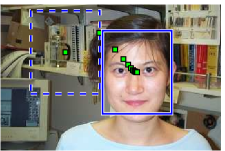
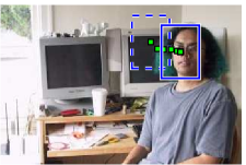
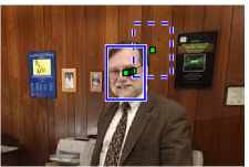
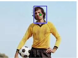
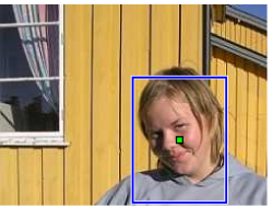
For the first experiment, we have trained a face representation model. $404$ faces cropped from CalTech-$101$ are used as positive raw images, and $1400$ negative images are randomly cropped from images which do not contain faces. The image size is reduced to $42\times 56$ pixels. Kernel-weighted RGB colour histograms, consisting of $16\times 16\times 16$ bins, are extracted for classification. By default we use a soft SVM trained with LIBSVM (slightly modified to use customized kernels). Test accuracy on the training data is $99.5\%~{}(1795/1804)$; and $91.7\%~{}(2752/3000)$ on a test data set which contains totally $3000$ negative data. Note that our main purpose is not to train a powerful face detector; rather, we want to obtain an appearance model that is more robust than the single-view appearance model. We now test how well the algorithm maximizes the SVM score. First, we feed the algorithm a rough initial guess and run MS. See Fig. 1 for details.

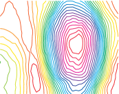
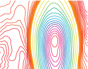
The first example in Fig. 1 comes from the training data set. The initial SVM score is negative. In this case, a single step is required to switch to a positive score—it moves closely to the target after one iteration. We plot the corresponding cost function in Fig. 2. By comparison, the cost function of the standard MS is also plotted (the target template is cropped from the same image). We can clearly see the difference. The other two test images are from outside of the training data set. Despite the significant face color difference and variation in illumination, our SVM localizer works well in both tests. To compare the robustness, we use the first face as a template to track the second face in Fig. 1, the standard MS tracker fails to converge to the true position.

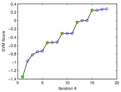
We now apply the global maximum seeking algorithm to object localization. In [2], it has been shown that it is possible to locate a target no matter from which initial position the MS tracker starts. Here we use the learned classification rule to determine when to stop searching. We start the annealed continuation procedure with the initial bandwidth $h_{0}=(42,56)$. Then the bandwidth pyramid works with the rule $h_{m+1}=\frac{h_{m}}{1.25}$, $m\in\{0,\cdots,M\}$. $M$ is the maximum number of iterations. We stop the search when for some $m$ the SVM score is positive upon convergence. The image center is set to be the initial position of the search for these $2$ tests. We present the results in Fig. 3.

In the first test, our proposed algorithm works well: It successfully finds the face location, and also the final bandwidth well fits the target. Fig. 3 (right) shows how the SVM score evolves. It can be seen that every bandwidth change significantly increases the score. If the target size is large and there is a significant overlap between the target and a search region at a coarse bandwidth, $h_{m}$, the overlap can make the cascade search stop prematurely (see the second test in Fig. 3). Again this problem is mainly caused by the color feature’s weak discriminative power. A remedy is to include more features. However, for certain applications where the scale-size is not critically important, our localization results have been usable. Furthermore, better results could be achieved when we train a model for a specific object (e.g., train an appearance model for a specific person) with a single color feature.

IV-B Tracking

Effectiveness of the proposed generalized kernel-based tracker is tested on a number of video sequences. We have compared with two popular color histogram based methods: the standard MS tracker [1] and particle filters [4].

Unlike the first experiment, we do not train an off-line SVM model for tracking. It is not easy to have a large amount of training data for a general object, therefore in the tracking experiment, an on-line SVM described in §II-C is used for training. The user crops several negative data and positive data for initial training. During the course of tracking the on-line SVM updates its model by regarding the tracked region as a positive example and randomly selecting a few sub-regions (background area) around the target as negative examples. A $16\times 16\times 16$-binned color histogram is used for both the generalized kernel tracker and standard MS tracker. For the particle filter, with $1000$ or $800$ particles, the tracker fails at the first a few frames. So we have used $1500$ particles.

Figure 4: Face sequence 1. Tracking results of the proposed tracker (top row); standard mean shift tracker (middle) and particle filtering (bottom row). Frames 26, 56, 318, 432 are shown. The video size is $320\times 240$ and the frame rate is $10$ frames per second (FPS).

Figure 5: Face sequence 2. Tracking results of the proposed tracker (top row); standard mean shift tracker (middle) and particle filtering (bottom row). Frames 86, 135, 204, 512 are shown. The video size is $320\times 240$ and the frame rate is $10$ FPS.

Figure 6: Walker sequence 1. Tracking results of the proposed generalized kernel tracker. Frames 20, 40, 60, 90, 115, 130 are shown. The video size is $384\times 288$ and the frame rate is $25$ FPS.

Figure 7: Walker sequence 2. Tracking results of the proposed generalized kernel tracker. Frames 10, 55, 80, 105, 140, 183 are shown. The video size and frame rate are same as Fig. 6.

Figure 8: Walker sequence 3. Tracking results of the proposed generalized kernel tracker. Frames 20, 98, 152, 220, 444, 553 are shown. The video is of size $352\times 288$ and frame rate $30$ FPS.

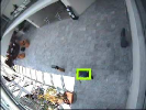
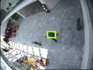
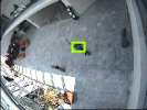
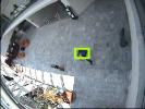
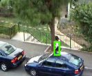
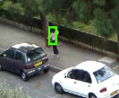
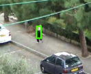
In the first experiment, the tracked person moves quickly. Hence the displacement between neighboring frames is large. The illumination also changes. The background scene is cluttered and contains materials with similar color as the target. The proposed algorithm tracks the whole sequence successfully. Fig. 4 summarizes the tracking results. The standard MS tracker fails at frame #57; recovers at frame #74 and then fails again. The particle filter also loses the target due to motion blur and fast movement. Our on-line adaptive tracker achieves the most accurate results.

Fig. 5 shows that the results on a more challenging video. The target turns around and at some frames it even moves out of the view. At frame #194, the target disappears. Generalized kernel tracker and particle filter recovers at the following frames while the MS tracker fails. Again we can see the proposed tracker performs best due to its learned template model and on-line adaptivity. When the head turns around, all trackers can lock the target because compared with the background, the hair color is more similar to the face color. These two experiments show the proposed tracker’s robustness to motion blur, large pose change and target’s fast movement over the standard MS tracker and particle filter based tracker. In the experiments, to initialize the proposed tracker, we randomly pick up a few negative samples from the background. We have found this simple treatment works well.

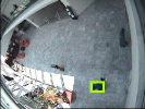
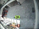
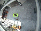
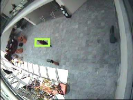
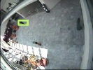
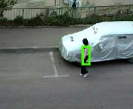
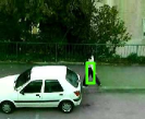
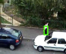
We present more samples from three more sequences in Figs. 6, 7 and 8. We mark only our tracker in these frames. From Figs. 6 and 7 we see that despite the target moving into shadow at some frames, our tracker successfully tracks the target through the whole sequences.

We have shown promising tracking results of the proposed tracker on several video clips. We now present some quantitative comparisons of our algorithm with other trackers.

First, we run the proposed tracker, MS, and particle filter trackers on the cubicle sequence 1. In Fig. 9, we show some tracking frames of our method and particle filtering. Compared with particle filtering, ours are much better in terms of accuracy and much faster in terms of the tracking speed. Our results are also slightly better than the standard MS tracker. But visually there is no significant difference, so we have not included MS results in Fig. 9.

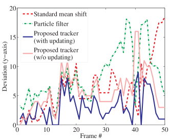
Again, the particle filter tracker uses $1500$ particles. We have run the particle filter $5$ times and the best result is reported. Fig. 10 shows the absolute deviation of the tracked object’s center at each frame. Clearly the generalized kernel tracker demonstrates the best result. We have reported the average tracking error (the Euclidean distance of the object’s center against the ground truth) in Table I, which shows the proposed tracker outperforms MS and particle filter. In Table I, the error variance estimates are calculated from the tracking results of all frames regardless the target is lost or not. We have also proved the importance of on-line SVM update. As mentioned, when we switch off the on-line update, our proposed tracker would behave similarly to the standard MS tracker. We see from Table I that even without updating, the generalized kernel tracker is slightly better than the standard MS tracker. This might be because the initialization schemes are different: the generalized kernel tracker can take multiple positive as well as negative training examples to learn an appearance model, while MS can only take a single image for initialization. Although we only use very few training examples (less than $10$), it is already better than the standard MS tracker. In this sequence, when the target object is occluded, the particle filter tracker only tracks the visible region such that the deviation becomes large. Our approach updates the learned appearance model using on-line SVM. The region that partially contains the occlusion is added to the object class database gradually based on the on-line update procedure. This way our tracker tracks the object position close to the ground truth.

We also report the tracking failure rate (FR) for this video, which is the percentage of the number of failure frames in the total number of frames. If the distance between the tracked center and the ground truth’s center is larger than a threshold, we mark it a failure. We have defined the threshold as $0.20$ or $0.25$ of the diagonal length of the ground truth’s bounding box, which results in two criteria: ${\rm FR}_{0.20}$ and ${\rm FR}_{0.25}$ respectively. The former is more strict than the latter. As shown in Table I, our tracker with on-line update produces lowest tracking failures under either criterion.

Figure 9: Cubicle sequence 1. Tracking results of the proposed tracker (top) and particle filtering (bottom). Frames 16, 30, 41, 45 are shown. The video is of size $352\times 288$ and $30$ FPS.

TABLE I: The average tracking error against the ground truth (pixels) on the cubicle sequence 1. The mean and standard deviation are reported. We also report the tracking failure rates.

	MS	Particle filter	Ours (w/o update)	Ours (update)
error	$9.6\pm 5.7$	$10.5\pm 5.8$	$8.5\pm 4.9$	$6.5\pm 2.8$
${\rm FR}_{0.20}$	44.0%	44.0%	28.0%	6.0%
${\rm FR}_{0.25}$	16.0%	34.0%	14.0%	0.0%

We also compare the running time of trackers, which is an important issue for real-time tracking applications. Table II reports the results on two sequences. The generalized kernel tracker (around $65$ fps) is comparable to the standard MS tracker, and much faster than the particle filter. This coincides with the theoretical analysis: our generalized kernel tracker’s computational complexity is independent of the number of support vectors, so in the test phrase, the complexity is almost same as the standard MS. One may argue that the on-line update procedure introduces some overhead. But the generalized kernel tracker employs the L-BFGS optimization algorithm which is about twice faster than MS, as shown in [2]. Therefore, overall, the generalized kernel tracker runs as fast as the MS tracker. Because the particle filter is stochastic, we have run it $5$ times and the average and standard deviation are reported. For our tracker and MS, they are deterministic and the standard deviation is negligible. Note that the computational complexity if the particle filter tracker is linearly proportional to the number of particles.

Figure 10: The $\ell_{1}$-norm absolute error (pixels) of the object’s center against the ground truth on the cubicle sequence 1. The two figures correspond to $x$-, and $y$-axis, respectively. The proposed tracker with on-line updating gives the best result. As expected, the proposed tracker without updating shows a similar performance with the standard MS tracker.

TABLE II: Running time per frame (seconds). The stochastic particle filter tracker has run $5$ times and the standard deviation is also reported.

Sequence	MS	Particle filter	Ours
cubicle 1	$0.0156$	$0.352\pm 0.025$	$0.0155$
walker 3	$0.0169$	$0.331\pm 0.038$	$0.0142$

We have run another test on cubicle sequence 2. We show some results of our method and particle filtering in Fig. 11. Although all the methods can track this sequence successfully, the proposed method achieves most accurate results. We see that when the tracked object turns around, our algorithm is still able to track it accurately. Table III summarizes the quantitative performance. Our method is also slightly better MS. Again we see that on-line update does indeed improve the accuracy. We have also reported the tracking failure rates on this video. Our tracker with on-line update has the lowest tracking failures and the one without on-line update is the second best. These results are consistent with the previous experiments.

TABLE III: The average tracking error against the ground truth (pixels) on the cubicle sequence 2. The mean and standard deviation are reported. We also report the tracking failure rates.

	MS	Particle filter	Ours (w/o update)	Ours (update)
error	$5.7\pm 3.5$	$8.4\pm 3.4$	$5.5\pm 3.2$	$4.2\pm 2.8$
${\rm FR}_{0.20}$	4.6%	15.4%	3.1%	0.0%
${\rm FR}_{0.25}$	0.0%	3.1%	0.0%	0.0%

Figure 11: Cubicle sequence 2. Tracking results of the proposed tracker (top) and particle filtering (bottom). Frames 9, 55, 60, 64 are shown. The video is of size $352\times 288$ and frame rate $30$ FPS.

Figure 12: The $\ell_{1}$-norm absolute error (pixels) of the object’s center against the ground truth on the walker sequence 3. The two figures correspond to $x$-, and $y$-axis, respectively. It clearly shows that on-line update of the generalized kernel tracker is beneficial: without on-line update, the error is larger.

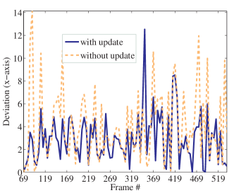
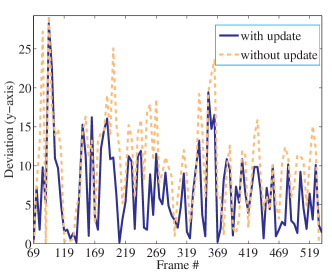
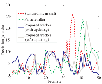
To demonstrate the effectiveness of the on-line SVM learning, we switch off the on-line update and run the tracker on the walker sequence 3. We plot the $\ell_{1}$-norm absolute deviation of the tracked object’s center in pixels at each frame in Fig. 12. Apparently, at most frames, on-line update produces more accurate tracking results. The average Euclidean tracking error is $8.0\pm 4.9$ pixels with on-line update and $12.7\pm 5.8$ pixels without on-line update.

Conclusions that we can draw from these experiments are: (1) The proposed generalized kernel-based tracker performs better than the standard MS tracker on all the sequences that we have used; (2) On-line learning often improves tracking accuracy.

V Conclusion

To summarize, we have proposed a novel approach to kernel based visual tracking, which performs better than conventional single-view kernel trackers [1, 13]. Instead of minimizing the density distance between the candidate region and the template, the generalized MS tracker works by maximizing the SVM classification score. Experiments on localization and tracking show its efficiency and robustness. In this way, we show the connection between standard MS tracking and SVM based tracking. The proposed method provides a generalized framework to the previous methods.

Future work will focus on the following possible avenues:

• Other machine learning approaches such as relevance vector machines (RVM) [42], might be employed to learn the representation model. Since in the test phrase, RVM and SVM take the same form, RVM can be directly used here. RVM achieves comparable recognition accuracy to the SVM, but requires substantially fewer kernel functions. It would be interesting to compare different approaches’ performances;

• The strategy in this paper can be easily plugged into a particle filter as an observation model. Improved tracking results are anticipated than for the simple color histogram particle filter tracker developed in [4].

Appendix

Generally Collins’ modified mean shift [30] (Equation (12)) cannot guarantee to converge to a local maximum. It is obvious that a fixed point ${\mathbf{x}}^{*}$ obtained by iteration using Equation (12) will not satisfy

$${\nabla}f({\mathbf{x}}^{*})=0.$$

$f(\cdot)$ is the original cost function. Therefore, generally, ${\mathbf{x}}^{*}$ will not even be an extreme point of the original cost function. In the following example, ${\mathbf{x}}^{*}$ obtained by Collins’ modified mean shift converges to a point which is close to a local minimum, but not the exact minimum.

Figure 13: With negative weights, the modified mean shift proposed in [30] may not be able to converge to the local maximum. In this case, it converges to a position close to a local minimum (not the exact minimum). The standard mean shift converges to the nearest minimum.

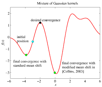
In Fig. 13 we give an example on a mixture of Gaussian kernel which contains some negative weights. In this case both the standard MS and Collins’ modified MS fail to converge to a maximum.

Chunhua Shen received the B.Sc. and M.Sc. degrees from Nanjing University, China, and the Ph.D. degree from University of Adelaide, Australia. He has been working as a research scientist in NICTA, Canberra Research Laboratory, Australia since October 2005. He is also an adjunct research follow at Australian National University and an adjunct lecturer at University of Adelaide. His research interests include statistical machine learning, convex optimization and their application in computer vision.

Junae Kim is a PhD student at the Research School of Information Sciences and Engineering, Australian National University. She is also attached to NICTA, Canberra Research Laboratory. She received the B.Sc. degree from Ewha Womans University, Korea in 2000, M.Sc. from Pohang University of Science and Technology, Korea in 2002, and M.Sc. from Australian National University in 2007. She was a researcher in Electronics and Telecommunications Research Institute (ETRI), Korea for 5 years before she moved to Australia. Her research interests include computer vision and machine learning.

Hanzi Wang received his B.Sc. degree in physics and M.Sc. degree in optics from Sichuan University, China, in 1996 and 1999, respectively. He received his Ph.D. degree in computer vision from Monash University, Australia, in 2004. He is a Senior Research Fellow at the School of Computer Science, University of Adelaide, Australia. His current research interest are mainly concentrated on computer vision and pattern recognition including robust statistics, model fitting, optical flow calculation, visual tracking, image segmentation, fundamental matrix estimation and related fields. He has published more than 30 papers in major international journals and conferences. He is a member of the IEEE society.

References

- [1] D. Comaniciu, V. Ramesh, and P. Meer, “Kernel-based object tracking,” IEEE Trans. Pattern Anal. Mach. Intell., vol. 25, no. 5, pp. 564–577, May 2003.
- [2] C. Shen, M. J. Brooks, and A. van den Hengel, “Fast global kernel density mode seeking: applications to localization and tracking,” IEEE Trans. Image Proce., vol. 16, no. 5, pp. 1457–1469, 2007.
- [3] W. Qu and D. Schonfeld, “Robust control-based object tracking,” IEEE Trans. Image Process., vol. 17, no. 9, pp. 1721–1726, 2008.
- [4] P. Pérez, C. Hue, J. Vermaak, and M. Gangnet, “Color-based probabilistic tracking,” in Proc. Eur. Conf. Comp. Vis., Copenhagen, Denmark, 2002, vol. 2350 of Lecture Notes in Computer Science, pp. 661–675.
- [5] C. Shen, A. van den Hengel, and A. Dick, “Probabilistic multiple cue integration for particle filter based tracking,” in Proc. Int. Conf. Digital Image Computing—Techniques & Applications, Sydney, Australia, 2003, pp. 309–408.
- [6] P. Pan and D. Schonfeld, “Dynamic proposal variance and optimal particle allocation in particle filtering for video tracking,” IEEE Trans. Circuits Syst. Video Technol., vol. 18, no. 9, pp. 1268–1279, 2008.
- [7] H. Wang, D. Suter, K. Schindler, and C. Shen, “Adaptive object tracking based on an effective appearance filter,” IEEE Trans. Pattern Anal. Mach. Intell., vol. 29, no. 9, pp. 1661–1667, 2007.
- [8] J. Lim, D. Ross, R.-S. Lin, and M.-H. Yang, “Incremental learning for visual tracking,” in Proc. Adv. Neural Inf. Process. Syst., Vancouver, Canada, 2004.
- [9] A. D. Jepson, D. J. Fleet, and T. F. El-Maraghi, “Robust online appearance models for visual tracking,” in Proc. IEEE Conf. Comp. Vis. Patt. Recogn., Kauai, 2001, vol. 1, pp. 415–422.
- [10] O. Javed, S. Ali, and M. Shah, “Online detection and classification of moving objects using progressively improving detectors,” in Proc. IEEE Conf. Comp. Vis. Patt. Recogn., San Diego, CA, 2005, vol. 1, pp. 696–701.
- [11] S. Avidan, “Ensemble tracking,” IEEE Trans. Pattern Anal. Mach. Intell., vol. 29, no. 2, pp. 261–271, 2007.
- [12] B. Han and L. Davis, “On-line density based appearance modeling for object tracking,” in Proc. IEEE Int. Conf. Comp. Vis., Beijing, China, 2005.
- [13] A. Elgammal, R. Duraiswami, and L. S. Davis, “Probabilistic tracking in joint feature-spatial spaces,” in Proc. IEEE Conf. Comp. Vis. Patt. Recogn., Madison, Wisconsin, 2003, vol. 1, pp. 781–788.
- [14] T. S. Jaakkola and D. Haussler, “Exploiting generative models in discriminative classifiers,” in Proc. Adv. Neural Inf. Process. Syst., 1998.
- [15] K. Tsuda, M. Kawanabe, G. Rätsch, S. Sonnenburg, and K.-R. Müller, “A new discriminative kernel from probabilistic models,” Neural Computation, vol. 14, no. 10, pp. 2397–2414, 2002.
- [16] P. J. Moreno, P. Ho, and N. Vasconcelos, “A Kullback-Leibler divergence based kernel for SVM classification in multimedia applications,” in Proc. Adv. Neural Inf. Process. Syst., Vancouver, Canada, 2003.
- [17] T. Jebara, R. Kondor, and A. Howard, “Probability product kernels,” J. Mach. Learn. Res., vol. 5, pp. 819–844, 2004.
- [18] S. Avidan, “Support vector tracking,” IEEE Trans. Pattern Anal. Mach. Intell., vol. 26, no. 8, pp. 1064–1072, 2004.
- [19] O. Williams, A. Blake, and R. Cipolla, “Sparse Bayesian learning for efficient visual tracking,” IEEE Trans. Pattern Anal. Mach. Intell., vol. 27, no. 8, pp. 1292–1304, 2005.
- [20] R. Jenssen, D. Erdogmus, J. C. Principe, and T. Eltoft, “Towards a unification of information theoretic learning and kernel methods,” in Proc. IEEE Workshop on Machine Learning for Signal Proce., Sao Luis, Brazil, 2004, pp. 93–102.
- [21] R. Jenssen, D. Erdogmus, J. C. Principe, and T. Eltoft, “The Laplacian PDF distance: A cost function for clustering in a kernel feature space,” in Proc. Adv. Neural Inf. Process. Syst., 2004, vol. 17, pp. 625–632.
- [22] G. Cauwenberghs and T. Poggio, “Incremental and decremental support vector machine learning,” in Proc. Adv. Neural Inf. Process. Syst., 2000, pp. 409–415.
- [23] G. Fung and O. L. Mangasarian, “Incremental support vector machine classification,” in Proc. SIAM Int. Conf. Data Mining, Arlington, VA, USA, 2002.
- [24] J. Kivinen, A. Smola, and R. C. Williamson, “Online learning with kernels,” IEEE Trans. Signal Proce., vol. 52, no. 8, pp. 2165–2176, 2004.
- [25] A. Bordes, S. Ertekin, J. Weston, and L. Bottou, “Fast kernel classifiers with online and active learning,” J. Mach. Learn. Res., vol. 6, pp. 1579–1619, 2005, http://leon.bottou.org/projects/lasvm.
- [26] V. Vapnik, The Nature of Statistical Learning Theory, Spinger Verlag, 1995.
- [27] C. Yang, R. Duraiswami, and L. Davis, “Efficient spatial-feature tracking via the mean-shift and a new similarity measure,” in Proc. IEEE Conf. Comp. Vis. Patt. Recogn., San Diego, CA, 2005, vol. 1, pp. 176–183.
- [28] A. B. Chan, N. Vasconcelos, and P. J. Moreno, “A family of probabilistic kernels based on information divergence,” SVCL-TR 2004/01, University of California, San Diego, 2004, http://www.svcl.ucsd.edu.
- [29] O. Chapelle, P. Haffner, and V. Vapnik, “SVMs for histogram based image classification,” IEEE Trans. Neural Networks, vol. 10, no. 5, pp. 1055–1064, 1999.
- [30] R. Collins, “Mean-shift blob tracking through scale space,” in Proc. IEEE Conf. Comp. Vis. Patt. Recogn., Madison, WI, USA, 2003, vol. 2, pp. 234–240.
- [31] B. Schölkopf, J. Platt, J. Shawe-Taylor, and A. Smola, “Estimating the support of a high-dimensional distribution,” Neural Computation, vol. 13, no. 7, pp. 1443–1471, 2001.
- [32] D. C. Liu and J. Nocedal, “On the limited memory method for large scale optimization,” Math. Programming B, vol. 45, no. 3, pp. 503–528, 1989.
- [33] T. Liu and H. Chen, “Real-time tracking using trust-region methods,” IEEE Trans. Pattern Anal. Mach. Intell., vol. 26, no. 3, pp. 397–402, March 2004.
- [34] I. Guskov, “Kernel-based template alignment,” in Proc. IEEE Conf. Comp. Vis. Patt. Recogn., New York, 2006, vol. 1, pp. 610–617.
- [35] T. Zhao and R. Nevatia, “Tracking multiple humans in crowded environment,” in Proc. IEEE Conf. Comp. Vis. Patt. Recogn., Washington, DC, USA, 2004, vol. 2, pp. 406–413.
- [36] T. Zhao, R. Nevatia, and B. Wu, “Segmentation and tracking of multiple humans in crowded environments,” IEEE Trans. Pattern Anal. Mach. Intell., 2008.
- [37] M. Dewan and G. D. Hager, “Toward optimal kernel-based tracking,” in Proc. IEEE Conf. Comp. Vis. Patt. Recogn., New York, USA, June 2006, vol. 1, pp. 618–625.
- [38] M.P. Wand and M.C. Jones, Kernel Smoothing, Chapman & Hall/CRC Press, 1995.
- [39] D. Comaniciu and P. Meer, “Mean shift: A robust approach toward feature space analysis,” IEEE Trans. Pattern Anal. Mach. Intell., vol. 24, no. 5, pp. 603–619, May 2002.
- [40] Z. Wu, “The effective energy transformation scheme as a special continuation approach to global optimization with application to molecular conformation,” SIAM J. Optimization, vol. 6, no. 3, pp. 748–768, 1996.
- [41] P. A. Viola and M. J. Jones, “Robust real-time face detection,” Int. J. Comp. Vis., vol. 57, no. 2, pp. 137–154, 2004.
- [42] M. Tipping, “Sparse Bayesian learning and the relevance vector machine,” J. Mach. Learn. Res., vol. 1, pp. 211–244, 2001.
![[Uncaptioned image]](/html/0905.2463/assets/x75.png) |