Time Delay Estimation from Low Rate Samples: A Union of Subspaces Approach

Abstract

Time delay estimation arises in many applications in which a multipath medium has to be identified from pulses transmitted through the channel. Various approaches have been proposed in the literature to identify time delays introduced by multipath environments. However, these methods either operate on the analog received signal, or require sampling at the Nyquist rate of the transmitted pulse. In this paper, our goal is to develop a unified approach to time delay estimation from low rate samples of the output of a multipath channel. Our methods result in perfect recovery of the multipath delays from samples of the channel output at the lowest possible rate, even in the presence of overlapping transmitted pulses. This rate depends only on the number of multipath components and the transmission rate, but not on the bandwidth of the probing signal. In addition, our development allows for a variety of different sampling methods. By properly manipulating the low-rate samples, we show that the time delays can be recovered using the well-known ESPRIT algorithm. Combining results from sampling theory with those obtained in the context of direction of arrival estimation methods, we develop sufficient conditions on the transmitted pulse and the sampling functions in order to ensure perfect recovery of the channel parameters at the minimal possible rate. Our results can be viewed in a broader context, as a sampling theorem for analog signals defined over an infinite union of subspaces.

I Introduction

Time delay estimation is an important signal processing problem, arising in various applications such as radar [1], underwater acoustics [2], wireless communications [3], and more. In a typical scenario, pulses with a priori known shape are transmitted through a multipath medium, which consists of several propagation paths. As a result the received signal is composed of delayed and weighted replicas of the transmitted pulses. In order to identify the medium, the time delay and gain coefficient of each multipath component has to be estimated from the received signal.

In this paper we consider recovery of the parameters defining such a multipath medium from samples of the channel output. Specifically, we assume that pulses with known shape are transmitted at a constant rate through the medium, and our aim is to recover the time delays and time-varying gain coefficients of each multipath component, from samples of the received signal. We focus on the sampling stage, and derive methods that ensure perfect recovery from samples of the channel output at the minimal possible rate. The proposed sampling schemes are flexible, so that a variety of different sampling techniques can be accommodated. Our main contribution is the development of efficient sampling schemes for the received signal. The resulting sampling rate is generally much lower than the traditional Nyquist rate of the transmitted pulses, and depends only on the number of multipath components and the transmission rate, but not on the bandwidth of the transmitted pulse. This can lead to significant sampling rate reduction, comparing to the Nyquist rate, in applications where only small number of propagation paths exists, or when the bandwidth of the transmitted pulse is relatively high. This reduction is desirable for practical implementation. Sampling at lower rates allows for analog-to-digital converters (ADCs) that are more precise (i.e. use more bits), and with lower power consumption. In addition, lowering the sampling rate can reduce the load on both hardware and further digital processing units.

A classical solution for the time delay estimation problem is based on correlation between the received signal and the transmitted pulse [1]. However, the time resolution of this method is limited by the inverse of the transmitted pulse bandwidth. Therefore, this technique is effective only when the multipath components are well separated in time, or when only one component is present. This approach was originally motivated in the analog domain, where the entire analog correlation is computed. Performing the correlation in the digital domain requires samples of the data at a high sampling rate, in order to approximate the continuous correlation.

In order to resolve closely spaced multipath components, various superresolution estimation algorithms were proposed. In [4, 5], the MUSIC [6] method was applied in the time domain in order to estimate the time delay of each multipath component. Hou and Wu [7] were the first to convert the time estimation problem to model-based sinusoidal parameter estimation, and used an autoregressive method in order to estimate the model’s parameters. Other works, such as [5, 8, 9], relied on the same principle, but different estimation algorithms were used: Tufts-Kumaresan SVD algorithm [10], TLS-ESPRIT method [11] and a modification of MUSIC, respectively.

In the above superresolution approaches, the sampling stage was typically not directly addressed. Most of these works rely on uniform pointwise samples of the received signal, at a high sampling rate. In [7] and [9] the required sampling rate is the Nyquist rate of the transmitted pulse. Since often the pulses are chosen to have small time support, the bandwidth can be quite large, corresponding to a high Nyquist rate. In [8] and in the frequency domain algorithm proposed in [5], the sampling of the received analog signal is not mentioned explicitly. Since these algorithms involve operations in the analog frequency domain, effectively they also require sampling at the Nyquist rate. The time domain algorithms proposed in [4] and [5] can theoretically recover the time delays from a low sampling rate, which depends on the number of multipath components. However, the sampling considerations were not directly addressed in these works, and no concrete conditions on the transmitted pulse and the samples were given, in order to ensure unique recovery of the delays from the samples.

Besides the sampling stage which is not studied in previous works, another assumption underlying all the methods above is that the receiver has access to a single experiment ([7, 8, 9]) or multiple non-overlapping experiments ([4, 5, 9]) on the channel. In each experiment a pulse is transmitted through the multipath medium, and it is required that all the returns vanish before the next experiment is conducted. This imposes the constraint that the transmitted pulse is sufficiently time limited, which can be problematic in certain scenarios. For example, in wireless communications, modulated pulses are transmitted at a constant symbol rate through the medium. In this case, we cannot consider the observed signal over one symbol period as an independent experiment, since it will generally be affected by reflections caused by adjacent symbols.

In Section II we propose a general signal model, that can describe the received signal from a time-varying multipath medium. An advantage of our model is that it does not require the assumption of non-overlapping experiments, and allows for general pulse shapes. We then formulate the medium identification problem as a sampling problem, in which the set of parameters defining the medium have to be recovered from samples of the received signal at the lowest possible rate. To this end we develop a general sampling scheme, which consists of filtering the received signal with a bank of $p$ sampling filters and uniformly sampling their outputs. This class of sampling methods is common in sampling theory [12] and can accommodate a wide variety of sampling techniques, including pointwise uniform sampling. Given $K$ multipath components, we show that at least $2K$ sampling filters are required in order to perfectly recover the time delays. We then develop explicit sampling strategies that achieve this minimal rate. In particular, we derive sufficient conditions on the transmitted pulse and the choice of sampling filters, which guarantee unique recovery of the channel parameters.

In order to recover the channel parameters from the given samples we combine results from standard sampling theory, with those of direction of arrival (DOA) algorithms [6, 11, 13, 14]. Specifically, by appropriate manipulation of the sampling sequences, we show that we can formulate our problem within the framework of DOA methods. We then rely on the estimation of signal parameters via rotational invariance techniques (ESPRIT) [11], developed in that context. The unknown delays are recovered from the samples by first applying a digital correction filter bank, and then applying the ESPRIT algorithm. Once the time delays are identified, the gain coefficients are recovered using standard sampling tools.

The sampling schemes we develop for the channel identification problem treated in this paper, can be viewed in the broader context of sampling theory. In Section V we discuss in detail the relationship between our problem and previous related setups treated in the sampling literature: sampling signals from a union of subspaces [15, 16], compressed sensing of analog signals [17, 18, 19, 20, 21, 22], and finite-rate of innovation (FRI) sampling [23, 24]. The results we develop here can be viewed as a special case of analog compressed sensing over an infinite union of spaces, and therefore extends previous work, which focused on finite unions, to a broader setting. In comparison with FRI techniques, our approach allows for lower sampling rates and at a lower computational cost. Furthermore, we do not need to impose stringent conditions on the pulse shapes, as required by FRI methods.

This paper is organized as follows. In Section II, we describe our signal model. A general sampling scheme of the received signal is proposed in Section III. Section IV describes the recovery of the unknown delays from the samples, and provides sufficient conditions ensuring a unique recovery. Relation to previous work is discussed in detail in Section V. Section VI describes an application example of channel identification in wireless communications. Numerical experiments are described in Section VII.

II Signal Model and Problem formulation

II-A Notations and Definitions

Matrices and vectors are denoted by bold font, with lowercase letters corresponding to vectors and uppercase letters to matrices. The $n$th element of a vector $\mathbf{a}$ is written as $\mathbf{a}_{n}$, and the $ij$th element of a matrix $\mathbf{A}$ is denoted by $\mathbf{A}_{ij}$. Superscripts $\left(\cdot\right)^{*}$, $\left(\cdot\right)^{T}$ and $\left(\cdot\right)^{H}$ represent complex conjugation, transposition and conjugate transposition, respectively. The Moore-Penrose pseudo-inverse of a matrix $\mathbf{A}$ is written as $\mathbf{A}^{\dagger}$. The identity matrix of size $n$ is denoted by $\mathbf{I}_{n}$.

The Fourier transform of a continuous-time signal $x\left(t\right)\in L_{2}$ is defined by $X\left(\omega\right)=\int_{-\infty}^{\infty}x\left(t\right)e^{-j\omega t}d\omega$, and

$$\left\langle x\left(t\right),y\left(t\right)\right\rangle=\int_{-\infty}^{\infty}x\left(t\right)y^{*}\left(t\right)dt,$$ (1)

denotes the inner product between two continuous-time signals. The discrete-time Fourier transform (DTFT) of a sequence $a\left[n\right]\in\ell_{2}$ is defined by

$$A\left(e^{j\omega T}\right)=\sum_{n\in\mathbb{Z}}a\left[n\right]e^{-j\omega nT},$$ (2)

and is periodic with period $2\pi/T$.

II-B Signal model

We consider the class of signals that can be written in the form

$$x\left(t\right)=\sum_{k=1}^{K}\sum_{n\in\mathbb{Z}}a_{k}\left[n\right]g\left(t-t_{k}-nT\right),$$ (3)

where $\tau=\left\{t_{k}\right\}_{k=1}^{K}$ is a set of $K$ distinct unknown time delays in the continuous interval $\left[0,T\right)$, $a_{k}\left[n\right]$ is an arbitrary sequence in $\ell_{2}$, and $g\left(t\right)\in L_{2}$ is a known function. Each signal from this class can describe the propagation of a pulse with known shape $g\left(t\right)$ which is transmitted at a constant rate of $1/T$ through a medium consisting of $K$ paths. Each path has a constant delay $t_{k}$, and a time-varying gain, which is described by the sequence $a_{k}\left[n\right]$. In cases where the transmitted pulses are amplitude modulated, the sequence $a_{k}\left[n\right]$ describes the multiplication between the pulse amplitude and the gain coefficient of each path. In Section VI we will discuss more thoroughly an example of a communication signal transmitted through a multipath time-varying channel.

Our problem is to determine the delays $\tau$ and the gains $a_{k}[n]$ from samples of the received signal $x(t)$, at the minimal possible rate. Since these parameters uniquely define $x(t)$, our channel identification problem is equivalent to developing efficient sampling schemes for signals of the form (3), allowing perfect reconstruction of the signal from its samples.

The model (3) is more general than that described in previous work [7, 4, 5, 8, 9], which is based on single or multiple experiments on the medium. In each experiment the received signal is observed over a finite time window, which is synchronized to the transmission time of the pulse. More precisely, the received signal in the $n$th experiment is given by

$$x_{n}\left(t\right)=\sum_{k=1}^{K}a_{kn}g\left(t-t_{k}\right),\quad t\in\left[0,T\right),$$ (4)

where $t_{k}$ is the delay of the $k$th multipath component which is constant in all the experiments, and $a_{kn}$ is the gain coefficient of the $k$th multipath component at the $n$th experiment, which is generally varying from one experiment to another. This model can be seen as a special case of (3) with additional constraints on the pulse $g\left(t\right)$ and the transmission rate $1/T$. Indeed, we can write the received signal on the $n$th experiment as

$$x_{n}\left(t\right)=x\left(t-nT\right)\quad t\in\left[0,T\right),$$ (5)

if we require that

$$g\left(t-t_{k}-nT\right)=0\textrm{ for all }n\neq 0.$$ (6)

This requirement means that the pulse $g\left(t\right)$ has finite time support, and that the repetition period of the pulses $T$, is long enough such that all the reflections from one pulse vanish before the next pulse is transmitted. On the other hand, our signal model does not require these constraints, so that it can support infinite length pulses and allows interference between experiments.

III Sampling Scheme

III-A Known delays

Before we treat our sampling problem of signals of the form (3), we first consider a simpler setting in which the delays $t_{k}$ are known. In this case our signal model is a special case of the more general class of signals that lie in a shift-invariant (SI) subspace. For such signals classes, there are well known sampling schemes that guarantee perfect recovery at the minimal possible rate [12, 17, 25]. Below, we review the main results in this setting which will serve as a basis for our development in the case in which the delays are unknown.

A finitely-generated SI subspace of $L_{2}$ is defined as [26, 27, 28]

$$\mathcal{A}=\left\{x\left(t\right)=\sum_{k=1}^{K}\sum_{n\in\mathbb{Z}}a_{k}\left[n\right]g_{k}\left(t-nT\right):a_{k}\left[n\right]\in\ell_{2}\right\}.$$ (7)

The functions $g_{k}\left(t\right)$ are referred to as the generators of $\mathcal{A}$. In order to guarantee a unique stable representation of any signal $x\left(t\right)\in\mathcal{A}$ by coefficients $a_{k}\left[n\right]$, the generators $g_{k}\left(t\right)$ are typically chosen to form a Riesz basis of $\mathcal{A}$ [26, 27]. Clearly, the signal model in (3) is a special case of (7) with generators $g_{k}(t)$, obtained from $K$ delayed versions of $g\left(t\right)$:

$$g_{k}\left(t\right)=g\left(t-t_{k}\right),\quad 1\leq k\leq K.$$ (8)

One way to sample a signal of the form (7) is to use $K$ parallel sampling channels [17]. In each channel the signal is first filtered with an impulse response $s_{\ell}^{*}\left(-t\right)$, and then sampled uniformly at times $t=nT$ to produce the sampling sequence $c_{\ell}\left[n\right]$, as depicted in the left-hand side of Fig. 1. The sampling sequence at the output of the $\ell$th channel can be written as

$$c_{\ell}\left[n\right]=\left\langle x\left(t\right),s_{\ell}\left(t-nT\right)\right\rangle,\quad 1\leq\ell\leq K.$$ (9)

By analyzing the DTFTs $C_{\ell}\left(e^{j\omega T}\right)$ of the sequences $c_{\ell}[n],1\leq\ell\leq K$, it was shown in [17] that the sequences $a_{\ell}\left[n\right],1\leq\ell\leq K$, which define the signal $x\left(t\right)$, can be recovered from $c_{\ell}[n]$ using an adequate multichannel filter bank. Specifically, let $\mathbf{c}\left(e^{j\omega T}\right),\mathbf{a}\left(e^{j\omega T}\right)$ denote the length-$K$ column vectors whose $\ell$th elements are $C_{\ell}\left(e^{j\omega T}\right),A_{\ell}\left(e^{j\omega T}\right)$ respectively. Then, it can be shown that

$$\mathbf{c}\left(e^{j\omega T}\right)=\mathbf{M}_{SG}\left(e^{j\omega T}\right)\mathbf{a}\left(e^{j\omega T}\right),$$ (10)

where $\mathbf{M}_{SG}\left(e^{j\omega T}\right)$ is a $K\times K$ matrix with $\ell k$th element

$$\Phi_{S_{\ell}G_{k}}\left(e^{j\omega T}\right)=\frac{1}{T}\sum_{m\in\mathbb{Z}}S_{\ell}^{*}\left(\omega-\frac{2\pi}{T}m\right)G_{k}\left(\omega-\frac{2\pi}{T}m\right).$$ (11)

Here $G_{k}\left(\omega\right)$ and $S_{\ell}\left(\omega\right)$ denote the Fourier transforms of $g_{k}\left(t\right)$ and $s_{\ell}\left(t\right)$ respectively. If this matrix is stably invertible a.e in $\omega$, then the sequences $a_{\ell}\left[n\right]$ can be recovered from the samples using the multichannel filter bank whose frequency response is given by $\mathbf{M}_{SG}^{-1}\left(e^{j\omega T}\right)$, as depicted in the right-hand side of Fig. 1.

The proposed sampling scheme achieves an average sampling rate of $K/T$ since there are $K$ sampling sequences each at rate $1/T$. Intuitively, this approach requires one sample per degree of freedom of the signal $x\left(t\right)$: for a signal of the form (3), under the assumption that the time delays are known, or a signal of the form (7), in each time period $T$ there are $K$ new parameters.

Figure 1: Sampling and reconstruction scheme for the case of known delays

III-B Unknown delays

We now address our original problem of designing a sampling scheme for signals of the form (3) with unknown delays. We propose a system similar to that used in the case of known delays, comprised of parallel sampling channels. Since now there are more degrees of freedom in the signal $x\left(t\right)$, intuitively we will require at least the same number of channels as in the case of known delays. Denoting the number of channels by $p$, this implies that $p\geq K$. As we will see, under certain conditions on the sampling filters and pulse $g(t)$, $p=2K$ sampling filters are sufficient to guarantee perfect recovery of $x(t)$ from the samples. We will also show that this is the minimal possible rate achievable for all signals $x(t)$.

In each channel of our sampling system the signal $x\left(t\right)$ is pre-filtered using the filter $s_{\ell}^{*}\left(-t\right)$ and sampled uniformly at times $t=nT$ resulting in the samples (9). In the Fourier domain, we can write (9) as

$$C_{\ell}\left(e^{j\omega T}\right)=\frac{1}{T}\sum_{m\in\mathbb{Z}}S_{\ell}^{*}\left(\omega-\frac{2\pi}{T}m\right)X\left(\omega-\frac{2\pi}{T}m\right).$$ (12)

From the definition of $x(t)$, its Fourier transform can be written as

$$X\left(\omega\right) = \sum_{k=1}^{K}\sum_{n\in\mathbb{Z}}a_{k}\left[n\right]G\left(\omega\right)e^{-j\omega\left(t_{k}+nT\right)}$$ (13)

$$= \sum_{k=1}^{K}A_{k}\left(e^{j\omega T}\right)G\left(\omega\right)e^{-j\omega t_{k}},$$

where $A_{k}\left(e^{j\omega T}\right)$ denotes the DTFT of the sequence $a_{k}\left[n\right]$, and $G\left(\omega\right)$ denotes the Fourier transform of $g\left(t\right)$. Substituting (13) into (12), we have

$$C_{\ell}\left(e^{j\omega T}\right) = \sum_{k=1}^{K}A_{k}\left(e^{j\omega T}\right)\frac{1}{T}\sum_{m\in\mathbb{Z}}S_{\ell}^{*}\left(\omega-\frac{2\pi}{T}m\right)$$ (14)

$$\cdot G\left(\omega-\frac{2\pi}{T}m\right)e^{-j\left(\omega-\frac{2\pi}{T}m\right)t_{k}}$$

$$= \sum_{k=1}^{K}A_{k}\left(e^{j\omega T}\right)e^{-j\omega t_{k}}\frac{1}{T}\sum_{m\in\mathbb{Z}}S_{\ell}^{*}\left(\omega-\frac{2\pi}{T}m\right)$$

$$\cdot G\left(\omega-\frac{2\pi}{T}m\right)e^{j\frac{2\pi}{T}mt_{k}},$$

where the first equality is a result of the fact that $A_{k}\left(e^{j\omega T}\right)$ is $2\pi/T$-periodic.

From now on, we will assume that $\omega\in\left[0,\frac{2\pi}{T}\right)$, and all the expressions in the DTFT domain are $2\pi/T$ periodic. Denoting by $\mathbf{c}\left(e^{j\omega T}\right)$ the length-$p$ column vector whose $\ell$th element is $C_{\ell}\left(e^{j\omega T}\right)$ and by $\mathbf{a}\left(e^{j\omega T}\right)$ the length-$K$ column vector whose $k$th element is $A_{k}\left(e^{j\omega T}\right)$, we can write (14) in matrix form as

$$\mathbf{c}\left(e^{j\omega T}\right)=\mathbf{M}\left(e^{j\omega T},\tau\right)\mathbf{D}\left(e^{j\omega T},\tau\right)\mathbf{a}\left(e^{j\omega T}\right).$$ (15)

Here $\mathbf{M}\left(e^{j\omega T},\tau\right)$ is a $p\times K$ matrix with $\ell k$th element

$$\mathbf{M}_{\ell k}\left(e^{j\omega T},\tau\right) = \frac{1}{T}\sum_{m\in\mathbb{Z}}S_{\ell}^{*}\left(\omega-\frac{2\pi}{T}m\right)$$ (16)

$$\cdot G\left(\omega-\frac{2\pi}{T}m\right)e^{j\frac{2\pi}{T}mt_{k}},$$

and $\mathbf{D}\left(e^{j\omega T},\tau\right)$ is a diagonal matrix with $k$th diagonal element equal to $e^{-j\omega t_{k}}$. Defining the vector $\mathbf{b}\left(e^{j\omega T}\right)$ as

$$\mathbf{b}\left(e^{j\omega T}\right)\mathbf{\mathit{=}D}\left(e^{j\omega T},\tau\right)\mathbf{a}\left(e^{j\omega T}\right),$$ (17)

we can rewrite (15) in the form

$$\mathbf{c}\left(e^{j\omega T}\right)=\mathbf{M}\left(e^{j\omega T},\tau\right)\mathbf{b}\left(e^{j\omega T}\right).$$ (18)

Our problem can then be reformulated as that of recovering $\mathbf{b}\left(e^{j\omega T}\right)$ and the unknown delay set $\tau$ from the vectors $\mathbf{c}\left(e^{j\omega T}\right)$, for all $\omega\in\left[0,\frac{2\pi}{T}\right)$. Once these are known, the vectors $\mathbf{a}\left(e^{j\omega T}\right)$ can be recovered using the relation in (17).

To proceed, we focus our attention on sampling filters $S_{\ell}(\omega)$ with finite support in the frequency domain, contained in the frequency range

$$\mathcal{F}=\left[\frac{2\pi}{T}\gamma,\frac{2\pi}{T}\left(p+\gamma\right)\right],$$ (19)

where $\gamma\in\mathbb{Z}$ is an index which determines the working frequency band $\mathcal{F}$. This choice should be such that it matches the frequency occupation of $g\left(t\right)$ (although $g(t)$ does not have to be bandlimited). This freedom allows our sampling scheme to support both complex and real valued signals. Under this choice of filters, each element $\mathbf{M}\left(e^{j\omega T},\tau\right)$ of (16) can be expressed as

$$\mathbf{M}_{\ell k}\left(e^{j\omega T},\tau\right)=\sum_{m=1}^{p}\mathbf{W}_{\ell m}\left(e^{j\omega T}\right)\mathbf{N}_{mk}\left(\tau\right),$$ (20)

where $\mathbf{W}\left(e^{j\omega T}\right)$ is a $p\times p$ matrix whose $\ell m$th element is given by

$$\mathbf{W}_{\ell m}\left(e^{j\omega T}\right) = \frac{1}{T}S_{\ell}^{*}\left(\omega+\frac{2\pi}{T}\left(m-1+\gamma\right)\right)$$ (21)

$$\cdot G\left(\omega+\frac{2\pi}{T}\left(m-1+\gamma\right)\right),$$

and $\mathbf{N}\left(\tau\right)$ is a $p\times K$ Vandermonde matrix with $mk$th element

$$\mathbf{N}_{mk}\left(\tau\right)=e^{-j\frac{2\pi}{T}\left(m-1+\gamma\right)t_{k}}.$$ (22)

Substituting (20) into (18),

$$\mathbf{c}(e^{j\omega T})=\mathbf{W}\left(e^{j\omega T}\right)\mathbf{N}\left(\tau\right)\mathbf{b}(e^{j\omega T}).$$ (23)

If $\mathbf{W}\left(e^{j\omega T}\right)$ is stably invertible, then we can define the modified measurement vector $\mathbf{d}\left(e^{j\omega T}\right)$ as

$$\mathbf{d}\left(e^{j\omega T}\right)=\mathbf{W}^{-1}\left(e^{j\omega T}\right)\mathbf{c}\left(e^{j\omega T}\right).$$ (24)

This vector satisfies

$$\mathbf{d}\left(e^{j\omega T}\right)=\mathbf{N}\left(\tau\right)\mathbf{b}\left(e^{j\omega T}\right).$$ (25)

Since $\mathbf{N}\left(\tau\right)$ is independent of $\omega$, from the linearity of the DTFT, we can express (25) in the time domain as

$$\mathbf{d}\left[n\right]=\mathbf{N}\left(\tau\right)\mathbf{b}\left[n\right],\quad n\in\mathbb{Z}.$$ (26)

The elements of the vectors $\mathbf{d}\left[n\right]$ and $\mathbf{b}\left[n\right]$ are the discrete time sequences, obtained from the inverse DTFT of the elements of the vectors $\mathbf{b}\left(e^{j\omega T}\right)$ and $\mathbf{d}\left(e^{j\omega T}\right)$ respectively.

Equation (25) and its equivalent time domain representation (26), describe an infinite set of measurement vectors, each obtained by the same measurement matrix $\mathbf{N}\left(\tau\right)$, which depends on the unknown delays $\tau$. This problem is reminiscent of the type of problems that arise in the field of DOA estimation [14], as we discuss in the next section. One class of efficient methods for DOA recovery, are known as subspace methods [14]. These techniques have subsequently been applied to many other problems such as spectral estimation [29], system identification [30] and more. Our approach is to rely on these methods in order to first recover $\tau$ from the measurements. After $\tau$ is known, the vectors $\mathbf{b}\left(e^{j\omega T}\right)$ and $\mathbf{a}\left(e^{j\omega T}\right)$ can be found using linear filtering relations by

$$\mathbf{b}\left(e^{j\omega T}\right)=\mathbf{N^{\dagger}}\left(\tau\right)\mathbf{d}\left(e^{j\omega T}\right).$$ (27)

Since $\mathbf{N}\left(\tau\right)$ is a Vandermonde matrix, its columns are linearly independent, and consequently $\mathbf{N^{\dagger}\mathbf{N}}=\mathbf{I}_{K}$. Using (17),

$$\mathbf{a}\left(e^{j\omega T}\right)=\mathbf{D}^{-1}\left(e^{j\omega T},\tau\right)\mathbf{N^{\dagger}}\left(\tau\right)\mathbf{d}\left(e^{j\omega T}\right).$$ (28)

The resulting sampling and reconstruction scheme is depicted in Fig. 2.

Figure 2: Sampling and reconstruction scheme for the case of unknown delays

Our last step, therefore, is to derive conditions on the filters $s_{\ell}^{*}\left(-t\right)$ and the function $g\left(t\right)$ in order that the matrix $\mathbf{W}\left(e^{j\omega T}\right)$ is stably invertible. To this end, we can decompose the matrix $\mathbf{W}\left(e^{j\omega T}\right)$ as

$$\mathbf{W}\left(e^{j\omega T}\right)=\mathbf{S}\left(e^{j\omega T}\right)\mathbf{G}\left(e^{j\omega T}\right)$$ (29)

where $\mathbf{S}\left(e^{j\omega T}\right)$ is a $p\times p$ matrix with $\ell m$th element

$$\mathbf{S}_{\ell m}\left(e^{j\omega T}\right)=\frac{1}{T}S_{\ell}^{*}\left(\omega+\frac{2\pi}{T}\left(m-1+\gamma\right)\right)$$ (30)

and $\mathbf{G}\left(e^{j\omega T}\right)$ is a $p\times p$ diagonal matrix whose $m$th diagonal element is given by

$$\mathbf{G}_{mm}\left(e^{j\omega T}\right)=G\left(\omega+\frac{2\pi}{T}\left(m-1+\gamma\right)\right).$$ (31)

Each one of these matrices needs to be stably invertible. Therefore, from (31) the condition that the function $g\left(t\right)$ needs to satisfy is that

$$0<a\leq\left|G\left(\omega\right)\right|\leq b<\infty\textrm{ a.e }\omega\in\mathcal{F}.$$ (32)

In addition the filters $s_{\ell}^{*}\left(-t\right)$ should be chosen in such a way that they form a stably invertible matrix $\mathbf{S}\left(e^{j\omega T}\right)$. Examples of such filters are given in the next subsection.

We note here that the conditions given above guarantee a stable digital correction filter bank $\mathbf{W}^{-1}\left(e^{j\omega T}\right)$, however generally it will be comprised of infinite length digital filters. Practical implementation of these filters can be achieved by truncating the impulse response. The length of the resulting filters will affect the total delay of our proposed method, which will generally be longer than that of the methods described in Section I, due to the additional digital filtering stage.

We summarize the results so far in the following proposition.

Proposition 1

Let $c_{\ell}\left[n\right]=\left\langle x\left(t\right),s_{\ell}\left(t-nT\right)\right\rangle,\;1\leq\ell\leq p$ be a set of $p$ sequences obtained by filtering the signal $x\left(t\right)$ defined by (3) with $p$ filters $s_{\ell}^{*}\left(-t\right)$ and sampling their outputs at times $nT$. Let $S_{\ell}(\omega)$ be supported on $\mathcal{F}=\left[\frac{2\pi}{T}\gamma,\frac{2\pi}{T}\left(p+\gamma\right)\right]$, and let $\Omega=[0,\frac{2\pi}{T})$. If the function $g\left(t\right)$ satisfies the condition in (32) and the matrix $\mathbf{S}\left(e^{j\omega T}\right)$, defined by (30), is stably invertible a.e $\omega\in\Omega$, then the delays $\tau$ and vector $\mathbf{b}\left(e^{j\omega T}\right)$ can be found from the set of equations

$$\mathbf{d}\left(e^{j\omega T}\right)=\mathbf{N}(\tau)\mathbf{b}\left(e^{j\omega T}\right),$$ (33)

using subspace methods, described in the next section. Here $\mathbf{N}\left(\tau\right)$ is a $p\times K$ Vandermonde matrix with $mk$th element $e^{-j\frac{2\pi}{T}\left(m-1+\gamma\right)t_{k}}$, and

$$\mathbf{d}\left(e^{j\omega T}\right)=\mathbf{W}^{-1}\left(e^{j\omega T}\right)\mathbf{c}\left(e^{j\omega T}\right),$$ (34)

with $\mathbf{W}\left(e^{j\omega T}\right)$ defined by (21). The sequences $a_{\ell}[n]$ can then be recovered by

$$\mathbf{a}\left(e^{j\omega T}\right)=\mathbf{D}^{-1}\left(e^{j\omega T},\tau\right)\mathbf{N}^{\dagger}(\tau)\mathbf{d}\left(e^{j\omega T}\right),\quad\omega\in\Omega$$ (35)

where $\mathbf{D}(e^{j\omega T,\tau})$ is a diagonal matrix with diagonal elements $e^{-j\omega t_{k}}$.

III-C Examples of filters

We now provide some examples of filters $s_{\ell}\left(t\right)$ satisfying the required conditions.

III-C1 Complex bandpass filter-bank

The first example is a set of complex bandpass filters. We assume that the working band is $\mathcal{F}=\left[0,\frac{2\pi}{T}p\right]$ ($\gamma=0)$, and the function $g\left(t\right)$ satisfies (32) on that frequency range. We choose the filters $s_{\ell}^{*}\left(-t\right)$ as ideal bandpass filters, covering consecutive frequency bands:

$$S_{\ell}\left(\omega\right)=\begin{cases}T,&\omega\in\left[\left(\ell-1\right)\frac{2\pi}{T},\ell\frac{2\pi}{T}\right]\\ 0,&\textrm{otherwise.}\end{cases}$$ (36)

The resulting matrix $\mathbf{S}\left(e^{j\omega T}\right)$ is diagonal, and stably invertible. This example generalizes to any valid working band, given by (19), by shifting the frequency response of the filters.

We now provide an example demonstrating the importance of the sampling filter.

Example 1

We consider the case where $g(t)=\delta(t)$ and there are $K=2$ diracs per period of $T=1$, as illustrated in Fig. 3(a). The sampling scheme described above, consisting of a complex bandpass filter-bank, is used. In Figs. 3(b)–(d), we show the outputs of the first $3$ sampling channels. This example demonstrates the need for the sampling filters when sampling short-length pulses at a low sampling rate. The sampling kernels have the effect of smoothing the short pulses (diracs in this example). Consequently, even when the sampling rate is low, the samples contain information about the signal. In contrast, if we were to sample the signal in Fig. 3(a) directly at a low rate, then we would often obtain only zero samples which contain no information about the signal.

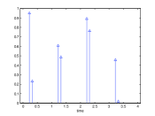
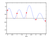
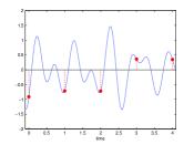
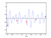
Figure 3: Stream of diracs. (a) $K=2$ diracs per period $T=1$. (b)-(d) The outputs of the first three sampling channels. The dashed lines denote the sampling instants.

III-C2 Delayed channels

In this example we assume $p$ is even and define the working band as

$$\mathcal{F}=\left[-\frac{\pi}{T}p,\frac{\pi}{T}p\right]$$ (37)

($\gamma=-p/2)$. We also assume that $g\left(t\right)$ satisfies (32). We choose the $\ell$th filter as a delay of $\Delta_{\ell}\in\left[0,T\right)$ followed by an ideal low pass filter. Thus,

$$S_{\ell}\left(\omega\right)=\begin{cases}Te^{-j\omega\Delta_{\ell}},&\omega\in\mathcal{F}\\ 0,&\textrm{otherwise.}\end{cases}$$ (38)

With this choice of filters, the $\ell m$th element of the matrix $\mathbf{S}\left(e^{j\omega T}\right)$ defined in (30) is given by

$$\mathbf{S}_{\ell m}\left(e^{j\omega T}\right) = e^{j\left(\omega+\frac{2\pi}{T}\left(m-1-p/2\right)\right)\Delta_{\ell}}$$ (39)

$$= e^{j\left(\omega-\frac{2\pi}{T}\left(p/2\right)\right)\Delta_{\ell}}e^{j\frac{2\pi}{T}\left(m-1\right)\Delta_{\ell}}.$$

The matrix $\mathbf{S}\left(e^{j\omega T}\right)$ can be expressed as

$$\mathbf{S}\left(e^{j\omega T}\right)=\mathbf{\Phi}\left(e^{j\omega T}\right)\mathbf{F},$$ (40)

where $\mathbf{\Phi}\left(e^{j\omega T}\right)$ is a diagonal $p\times p$ matrix whose $\ell$th diagonal element is $e^{j\left(\omega-\frac{2\pi}{T}\left(p/2\right)\right)\Delta_{\ell}}$, and $\mathbf{F}$ is a Vandermonde matrix whose $\ell m$th element is given by $e^{j\frac{2\pi}{T}\left(m-1\right)\Delta_{\ell}}$. From (40) it can be seen that $\mathbf{S}\left(e^{j\omega T}\right)$ is invertible for all $\omega\in\Omega$, when the delays in each channel $\Delta_{\ell}$ are distinct.

One special case of this choice of sampling filters is when the delays are uniformly spaced, i.e $\Delta_{\ell}=\left(\ell-1\right)T/p$. In this case our sampling scheme can be implemented by an ideal low pass filter with cutoff $\pi p/T$, followed by a uniform sampler at a rate of $p/T$.

IV Recovery of the Unknown Delays

We have seen in the previous section that perfect reconstruction of a signal $x\left(t\right)$ of the form (3), is equivalent to that of recovering the delays $\tau$ from the modified measurements of (26). As we now show, this problem is similar to that arising in DOA estimation.

IV-A Relation to direction of arrival estimation

In DOA estimation [6, 11, 13, 14], $K$ narrow band sources impinge on an array, composed of $p$ sensors, from distinct DOAs. The goal is to estimate the DOAs of the sources from a set of $M$ measurements, obtained from the sensors outputs at distinct time instants.

The DOA estimation problem can be formulated using the following measurement model

$$\boldsymbol{X}=\boldsymbol{A}\left(\Theta\right)\mathbf{S}$$ (41)

where $\boldsymbol{X}$ is a $p\times M$ matrix, composed of the measurements in its columns, $\mathbf{S}$ is a $K\times M$ matrix consisting of the sources signals in its columns and $\boldsymbol{A}\left(\Theta\right)$ is a $p\times K$ matrix which depends on the set of unknown DOAs $\Theta$. The structure of $\boldsymbol{A}\left(\Theta\right)$ is such that its $k$th column, denoted $\mathbf{a}\left(\theta_{k}\right)$, depends only on the DOA $\theta_{k}$ of the $k$th source. The vector $\mathbf{a}\left(\theta_{k}\right)$ is referred to as the steering vector of the array toward direction $\theta_{k}$. The set containing all possible steering vectors, i.e, $\left\{\mathbf{a}\left(\theta\right),\theta\in\left[0,2\pi\right)\right\}$ is referred as the array manifold. Given $\boldsymbol{X}$, the problem is to recover the DOAs $\theta_{k}$, and the sources $\boldsymbol{S}$.

The set of equations in (26) has the same form as (41). The $k$th column of the matrix $\mathbf{N}\left(\tau\right)$ depends only on the $k$th unknown delay $t_{k}$, and can be described by the vector $\mathbf{n}\left(t_{k}\right)$, where

$$\mathbf{n}\left(t\right)=\left[\begin{array}[]{cccc}e^{-j\frac{2\pi}{T}\gamma t}&e^{-j\frac{2\pi}{T}\left(1+\gamma\right)t}&\cdots&e^{-j\frac{2\pi}{T}\left(p-1+\gamma\right)t}\end{array}\right]^{T}.$$ (42)

The array manifold in our setting is the set of vectors $\{\mathbf{n}(t),t\in[0,T)\}$. Therefore, we can adopt DOA methods to estimate the unknown delays. The only difference between the two problems is that in our setting, we have infinitely many measurement vectors, in contrast to the DOA problem in which $\boldsymbol{X}$ has finitely many columns. This will require several adjustments, which we will detail in the ensuing subsections.

Two prominent methods used for DOA estimation are MUSIC (MUltiple Signal Classification) [6] and ESPRIT (Estimation of Signal Parameters via Rotational Invariance Techniques) [11]. These algorithms belong to a class of techniques, known as subspace methods, which are based on separating the space containing the measurements into two subspaces, the signal and noise subspaces. Estimating the unknown set of parameters using MUSIC involves a continuous one-dimensional search over the parameter range. This procedure can be costly from a computational point of view. The ESPRIT approach can estimate the unknown set of parameters more efficiently, by imposing the additional requirement that the measurement matrix is rotationally invariant. We describe this property in subsection IV-C and show that in our case $\mathbf{N}\left(\tau\right)$ satisfies this condition, and therefore we use the ESPRIT approach.

We note that although the MUSIC and ESPRIT methods were originally developed as DOA estimators, these approaches and other subspace methods have been used successfully in other fields.

IV-B Sufficient conditions for perfect recovery

We now rely on results obtained in the context of DOA estimation in order to develop sufficient conditions for a unique solution to (26). Such a solution consists of the infinite set of vectors $\mathbf{b}\left[n\right],n\in\mathbb{Z}$ and the unknown delays $\tau.$

Conditions for a unique solution $\left(\Theta,\mathbf{S}\right)$ for (41) where derived in [31]. Since [31] deals with a finite number of measurements, we have to extend the results to our case, which consists of an infinite number of measurements. The analysis in [31] requires a preliminary condition that any subset of $p$ distinct steering vectors from the array manifold is linearly independent. In our case this condition translates into the requirement that any set of $p$ vectors $\mathbf{n}\left(t_{i}\right),1\leq i\leq p$ associated with distinct delays $t_{i}\in\left[0,T\right),1\leq i\leq p$ are linearly independent. From (42), any such set forms a $p\times p$ Vandermonde matrix, and are therefore linearly independent. Therefore, this condition automatically holds in our problem without forcing any additional constraints.

To derive sufficient conditions for a unique solution of the set of infinite equations (26) we introduce some notation. We define the measurement set $\mathbf{d}\left[\Lambda\right]$ as the set containing all measurement vectors $\mathbf{d}\left[\Lambda\right]=\left\{\mathbf{d}\left[n\right],n\in\mathbb{Z}\right\}$. Similarly, we define the unknown vector set $\mathbf{b}\left[\Lambda\right]$ as $\mathbf{b}\left[\Lambda\right]=\left\{\mathbf{b}\left[n\right],n\in\mathbb{Z}\right\}$. We may then rewrite (26) as

$$\mathbf{d}\left[\Lambda\right]=\mathbf{N}\left(\tau\right)\mathbf{b}\left[\Lambda\right].$$ (43)

The following proposition provides sufficient conditions for a unique solution to (43).

Proposition 2

If $\left(\bar{\tau},\bar{\mathbf{b}}\left[\Lambda\right]\right)$ is a solution to (43),

$$p>2K-\textrm{dim}\left(\textrm{span}\left(\bar{\mathbf{b}}\left[\Lambda\right]\right)\right)$$ (44)

and

$$\textrm{dim}\left(\textrm{span}\left(\bar{\mathbf{b}}\left[\Lambda\right]\right)\right)\geq 1,$$ (45)

then $\left(\bar{\tau},\bar{\mathbf{b}}\left[\Lambda\right]\right)$ is the unique solution of (43).

The notation $\textrm{span}\left(\bar{\mathbf{b}}\left[\Lambda\right]\right)$ is used for the minimal dimension subspace containing the unknown vector set $\bar{\mathbf{b}}\left[\Lambda\right]$. The condition (45) is needed to avoid the case where $\bar{\mathbf{b}}\left[\Lambda\right]=0.$ In this case clearly the set $\tau$ can not recovered uniquely.

Proof:

We denote $r=\textrm{dim}\left(\textrm{span}\left(\bar{\mathbf{b}}\left[\Lambda\right]\right)\right)$. From (45) $r\geq 1$. Therefore, there exist a finite subset $\tilde{\Lambda}=\left\{n_{i}\right\}_{i=1}^{r}\subset\Lambda$, such that the vector set $\bar{\mathbf{b}}\tilde{\left[\Lambda\right]}$ spans an $r$-dimensional subspace:

$$\textrm{dim}\left(\textrm{span}\left(\bar{\mathbf{b}}\tilde{\left[\Lambda\right]}\right)\right)=r.$$ (46)

By defining the matrices $\mathbf{B}$ and $\mathbf{D}$ as the matrices consisting of the vector sets $\bar{\mathbf{b}}\tilde{\left[\Lambda\right]}$ and $\bar{\mathbf{d}}\tilde{\left[\Lambda\right]}$, we can write

$$\mathbf{D}=\mathbf{N}\left(\bar{\tau}\right)\mathbf{B}.$$ (47)

Clearly, from its construction, the rank of the matrix $\mathbf{B}$ is $r$. From (44),

$$p>2K-r.$$ (48)

According to Theorem 1 in [31], the solution $\left(\bar{\tau},\mathbf{B}\right)$ is the unique solution to (47) under the condition (48).

Since the set of unknown delays $\bar{\tau}$ is the unique solution to the finite set of equations (47), it is also a unique solution to the infinite set of equations (43). Once $\bar{\tau}$ is uniquely determined, the matrix $\mathbf{N}\left(\bar{\tau}\right)$ is known. Since every vector of the vector set $\bar{\mathbf{b}}\tilde{\left[\Lambda\right]}$ is contained in $\mathbb{C}^{K}$,

$$\textrm{dim}\left(\textrm{span}\left(\bar{\mathbf{b}}\tilde{\left[\Lambda\right]}\right)\right)\leq K.$$ (49)

Therefore, according to (44) $p>K$. The matrix $\mathbf{N}\left(\bar{\tau}\right)$ is a $p\times K$ Vandermonde matrix which consist of $K$ linearly independent vectors. Therefore, for every $n\in\Lambda$, if $\bar{\mathbf{b}}\left[n\right]$ is a solution to

$$\mathbf{d}\left[n\right]=\mathbf{N}\left(\bar{\tau}\right)\mathbf{b}\left[n\right]$$ (50)

then it is the unique solution. ∎

Proposition 2 suggests that a unique solution to the set of equations (26) is guaranteed, under proper selection of the number of sampling channels $p$. This parameter, in turn, determines the average sampling rate of our sampling scheme, which is given by $p/T$. The condition (44) depends on the value of $\textrm{dim}\left(\textrm{span}\left(\mathbf{b}\left[\Lambda\right]\right)\right)$, which is generally not known in advance. According to our assumption $\textrm{dim}(\textrm{span}(\bar{\mathbf{b}}\tilde{[\Lambda]}))\geq 1$, therefore in order to satisfy the uniqueness condition (44) for every signal of the form (3), we must have $p>2K-1$ sampling channels or a minimal sampling rate of $2K/T$. Comparing this result to the minimal sampling rate in the case when the delays are known in advance, there is a penalty of $2$ in the minimal rate.

In Section V-A we show that our signal model, described in (3), can be considered as part of a more general framework of signals that lie in a union of SI subspaces [15]. It was shown in [15] that the theoretical minimum sampling rate required for perfect recovery of such a signal from its samples is $2K/T$. Therefore, according to the results of Proposition 2, our sampling scheme can achieve the minimal sampling rate required for signals of the form (3).

The minimal sampling rate of $2K/T$, which is achieved by our scheme, does not depend on the bandwidth of the pulse $g\left(t\right)$, but only on the number of propagation paths $K$. In applications where the number of propagation paths is relatively small, or the bandwidth of the transmitted pulse is high, our approach can provide a sampling rate lower than the Nyquist rate. More precisely, when $2K/T<W$, where $W$ is the bandwidth of transmitted pulse, our method can reduce the sampling rate relatively to the Nyquist rate. For example, the setup in [32], used for characterization of ultra-wide band (UWB) wireless indoor channels, consists of pulses with bandwidth of $W=1$GHz transmitted at a rate of $1/T=2$MHz. Under the assumption that there are $32$ significant multipath components, our method can reduce the sampling rate down to $128$MHz compared with the $2$GHz Nyquist rate.

Beside the theoretical interest, sampling rate reduction is also important for implementation considerations. For practical ADCs, which perform the sampling process, there is a trade-off between sampling rate and resolution [33]. Therefore, reducing the sampling rate allows the use of more precise ADCs, which can improve the time delay estimation. The power consumption of an ADC can also be reduced by lowering the sampling rate [33]. In addition, a lower rate leads to more efficient digital processing hardware, since a smaller number of samples has to be processed. This also allows performing the digital processing operations in real time.

IV-C Recovering the unknown delays

According to Proposition 2, in order be able to perfectly reconstruct every signal of the form (3), our sampling scheme must have $p\geq 2K$ sampling channels. We assume throughout that this condition holds.

We now describe an algorithm for the recovery of the unknown delays from the measurement set $\mathbf{d}\left[\Lambda\right]$, which is based on the ESPRIT [11] algorithm. One of the conditions needed in order to use the ESPRIT method is that the correlation matrix

$$\mathbf{R}_{bb}=\sum_{n\in\mathbb{Z}}\mathbf{b}\left[n\right]\mathbf{b}^{H}\left[n\right],$$ (51)

is positive definite. In order to relate this condition to our problem, we state the following proposition from [21].

Proposition 3

If the sum (51) exists, then every matrix $\mathbf{V}$ satisfying $\mathbf{R}_{bb}=\mathbf{V}\mathbf{V}^{H}$ has column span equal to $\textrm{span}\left(\mathbf{b}\left[\Lambda\right]\right)$.

An immediate corollary from Proposition 3 is that $\mathbf{R}_{bb}\succ 0$ is equivalent to the condition $\textrm{dim}\left(\textrm{span}\left(\mathbf{b}\left[\Lambda\right]\right)\right)=K$. In this case, which we refer to as the uncorrelated case, we can apply the ESPRIT algorithm on the measurement set $\mathbf{d}\left[n\right]$ in order to recover the unknown delays. The case $\textrm{dim}\left(\textrm{span}\left(\mathbf{b}\left[\Lambda\right]\right)\right)<K$, will be referred to as the correlated case. In this setting the condition $\mathbf{R}_{bb}\succ 0$ doest not hold, and the ESPRIT algorithm cannot applied directly. Instead, we will use an additional stage originally proposed in [34, 35].

Note, that

$$\mathbf{R}_{dd} = \sum_{n\in\mathbb{Z}}\mathbf{d}\left[n\right]\mathbf{d}^{H}\left[n\right]$$ (52)

$$= \mathbf{N}\left(\tau\right)\left(\sum_{n\in\mathbb{Z}}\mathbf{b}\left[n\right]\mathbf{b}^{H}\left[n\right]\right)\mathbf{N}^{H}\left(\tau\right)$$

$$= \mathbf{N}\left(\tau\right)\mathbf{R}_{bb}\mathbf{N}^{H}\left(\tau\right).$$

Since for any set of delays $t_{k}$, the matrix $\mathbf{N}\left(\tau\right)$ has full column-rank, the ranks of the matrices $\mathbf{R}_{dd}$ and $\mathbf{R}_{bb}$ are equal. Therefore, the decision whether we are in the uncorrelated or correlated case can made directly from the given measurements by forming the matrix $\mathbf{R}_{dd}$.

IV-C1 Uncorrelated Case

From (52), under the assumption that the matrix $\mathbf{R}_{bb}$ is positive definite, it can be shown that the rank of the matrix $\mathbf{R}_{dd}$ is $K$. Moreover, the matrices $\mathbf{R}_{dd}$ and $\mathbf{N}\left(\tau\right)$ have the same column span which is referred as the signal subspace. By performing a singular value decomposition (SVD) of the matrix $\mathbf{R}_{dd}$, we can obtain $K$ vectors, which span the signal subspace, by taking the $K$ left singular vectors associated to the non-zero singular values of $\mathbf{R}_{dd}$. We define the $p\times K$ matrix $\mathbf{E}_{s}$ as the matrix containing those vectors in its columns.

Now, we will the exploit the special structure of the Vandermonde matrix. We denote the matrix $\mathbf{N}_{\downarrow}\left(\tau\right)$ as the sub matrix extracted from $\mathbf{N}\left(\tau\right)$ by deleting its last row. In the same way we define $\mathbf{N}_{\uparrow}\left(\tau\right)$ as the sub matrix extracted from $\mathbf{N}\left(\tau\right)$ by deleting its first row. The Vandermonde matrix $\mathbf{N}\left(\tau\right)$ satisfies the following rotational invariance property:

$$\mathbf{N}_{\uparrow}\left(\tau\right)=\mathbf{N}_{\downarrow}\left(\tau\right)\mathbf{R}\left(\tau\right)$$ (53)

where $\mathbf{R}\left(\tau\right)$ is a diagonal $K\times K$ matrix, whose $k$th diagonal element is given by $\mathbf{R}_{kk}\left(\tau\right)=e^{-j2\pi t_{k}/T}$. Since the matrices $\mathbf{N}\left(\tau\right)$ and $\mathbf{E}_{s}$ have the same column span, there exists an invertible $K\times K$ matrix $\mathbf{T}$ such that

$$\mathbf{N}\left(\tau\right)=\mathbf{E}_{s}\mathbf{T}.$$ (54)

By deleting the last row in (54) we get

$$\mathbf{N}_{\downarrow}\left(\tau\right)=\mathbf{E}_{s\downarrow}\mathbf{T}.$$ (55)

Similarly, deleting the first row in (54) and using the rotational invariance property (53), we have

$$\mathbf{N}_{\downarrow}\left(\tau\right)\mathbf{R}\left(\tau\right)=\mathbf{E}_{s\uparrow}\mathbf{T}.$$ (56)

Combining (55) and (56) leads to the following relation between the matrices $\mathbf{\mathbf{E}_{s\uparrow}}$ and $\mathbf{E}_{s\downarrow}$:

$$\mathbf{\mathbf{E}_{s\uparrow}}=\mathbf{E}_{s\downarrow}\mathbf{T}\mathbf{R}\left(\tau\right)\mathbf{T}^{-1}.$$ (57)

The matrix $\mathbf{\mathbf{E}_{s\uparrow}}$ is a $\left(p-1\right)\times K$ ($p>K)$ matrix with full column rank. Therefore $\mathbf{E}_{s\downarrow}^{\dagger}\mathbf{\mathbf{E}_{s\uparrow}}=\mathbf{I}_{K}$. Using (57) we define the following $K\times K$ matrix $\mathbf{\Phi}$ as

$$\mathbf{\Phi=\mathbf{E}_{s\downarrow}^{\dagger}}\mathbf{\mathbf{E}_{s\uparrow}}=\mathbf{T}\mathbf{R}\left(\tau\right)\mathbf{T}^{-1}.$$ (58)

From (58) it is clear that the diagonal matrix $\mathbf{R}\left(\tau\right)$ can be obtained from the matrix $\mathbf{\Phi}$ by performing an eigenvalue decomposition. Once the matrix $\mathbf{R}\left(\tau\right)$ is known, the unknown delays can be retrieved from its diagonal elements as

$$t_{k}=-\frac{T}{2\pi}\textrm{arg}\left(\mathbf{R}_{kk}\left(\tau\right)\right).$$ (59)

In summary, our algorithm consist of the following steps:

1. Construct the correlation matrix $\mathbf{R}_{dd}=\sum_{n\in\mathbb{Z}}\boldsymbol{d}\left[n\right]\boldsymbol{d}^{H}\left[n\right]$.

2. Perform an SVD decomposition of $\mathbf{R}_{dd}$ and construct the matrix $\mathbf{E}_{s}$ consisting of the $K$ singular vectors associated with the non-zero singular values in its columns.

3. Compute the matrix $\mathbf{\Phi=\mathbf{E}_{s\downarrow}^{\dagger}}\mathbf{\mathbf{E}_{s\uparrow}}$.

4. Compute the eigenvalues of $\mathbf{\Phi}$, $\lambda_{i},i=1,2,\ldots,K$.

5. Retrieve the unknown delays by $t_{i}=-\frac{T}{2\pi}\textrm{arg}\left(\lambda_{i}\right)$.
   

IV-C2 Correlated Case

When the condition $\mathbf{R}_{bb}\succ 0$ is not satisfied the ESPRIT algorithm cannot be applied directly on the vector set $\mathbf{d}\left[\Lambda\right]$. In this case the rank of $\mathbf{R}_{dd}$ is smaller than $K$, and therefore its column span is no longer equal to the entire signal subspace. To accommodate this setting, we perform an additional stage before applying the ESPRIT method, based on the spatial smoothing technique proposed in [35, 34].

To proceed, we define $M=p-K$ length-$\left(K+1\right)$ sub vectors

$$\boldsymbol{d}_{i}\left[n\right]=\left[\begin{array}[]{cccc}d_{i}\left[n\right]&d_{i+1}\left[n\right]&\ldots&d_{i+K}\left[n\right]\end{array}\right]^{T}.$$ (60)

We define the smoothed correlation matrix $\overline{\mathbf{R}}_{dd}$ as

$$\mathbf{\overline{R}}_{dd}=\frac{1}{M}\sum_{i=1}^{M}\sum_{n\in\mathbb{Z}}\boldsymbol{d}_{i}\left[n\right]\boldsymbol{d}_{i}^{H}\left[n\right].$$ (61)

Under our assumptions $p\geq 2K$, therefore $M\geq K$. According to [35], when $M\geq K$ the rank of the smoothed correlation matrix is $K$ regardless of the rank of the matrix $\mathbf{R}_{bb}$. We will refer now to column rank of $\overline{\mathbf{R}}_{dd}$ as the signal subspace, and can then apply the ESPRIT algorithm on this matrix.

V Related Sampling Problems

In the introduction, we outlined previous approaches to time-delay estimation. In this section, we explore in more detail the relationship between our sampling problem and previous related setups treated in the sampling literature: sampling signals from a union of subspaces [15, 16], compressed sensing of analog signals [17, 18, 19, 20], and FRI sampling [23, 24].

V-A Sampling signals from a union of subspaces

A signal model which received growing interest recently is that of signals that lie in a union of subspaces [15, 16, 20, 18, 19, 22]. Under this model each signal $x\left(t\right)$ can be described as [15]

$$x\left(t\right)\in\bigcup_{\gamma\in\Gamma}\mathcal{S}_{\gamma},$$ (62)

where $\mathcal{S}_{\gamma}$ are subspaces of a given Hilbert space and $\Gamma$ is an index set. The signal $x(t)$ lies in one of the subspaces $\mathcal{S}_{\gamma}$, however it is not known in advance in which one. Thus, effectively, to determine $x(t)$, we first need to find the active subspace, or the index $\gamma$.

Our signal model, given by (3), can be formulated as in (62). As described in Subsection III-A once the time delays are fixed, each signal $x\left(t\right)$ lies in a SI subspace spanned by $K$ generators. Therefore, the set of all signals of the form (3) constitute an infinite union of SI subspaces, where $\gamma$ is the set of delays $\tau$, which can take on any continuous value in the interval $[0,T]$, and $\mathcal{S}_{\gamma}$ is the corresponding SI subspace.

In [15, 16] necessary and sufficient conditions are derived for a sampling operator to be invertible over a union of subspaces. For the case of a union of SI subspaces, [15] suggests a sampling scheme, similar to that used in [17] and in this paper, comprised of parallel sampling channels. Conditions on the sampling filters are then given in order to ensure reconstruction of the signals from its samples. In addition, the minimal number of sampling channels allowing perfect recovery of the signal from its samples is shown to be $2K$. This leads to a minimal sampling rate of $2K/T$ which is achieved by our scheme. However, in [15] no concrete reconstruction algorithms were given that can achieve this rate. Furthermore, although conditions for invertibility were provided, these do not necessarily imply that there exists an efficient recovery algorithm, which can recover the signal from its samples at the minimal rate. Our aim in this work, is to provide concrete recovery techniques, that are simple to implement, for signals over an infinite union of SI subspaces.

In summary, in this work we focus on a special case of signals that lie in an infinite union of SI subspaces. For this case, in contrast to [15], we provide a concrete reconstruction method. This method achieves the minimal theoretical sampling rate derived in [15]. In addition, while other works [20, 18, 19, 17, 22] provided reconstruction algorithms only for signals defined over a finite union of subspaces, here we provide a first systematic sampling and reconstruction method for signals in an infinite union of subspaces.

V-B Compressed sensing of analog signals

The sampling problem in [17] also deals with signals that lie in a union of SI spaces and provides recovery algorithms. However in the setting of [17] there are finite number of possible subspaces, in contrast to our case, where there are an infinite number of possible subspaces.

The signal model in [17] can be described in terms of $N$ generating functions $a_{\ell}(t)$ as

$$x\left(t\right)=\sum_{\left|\ell\right|=K}\sum_{n\in\mathbb{Z}}d_{\ell}\left[n\right]a_{\ell}\left(t-nT\right),$$ (63)

where the notation $\left|\ell\right|=K$ means a sum over at most $K$ elements. Thus, for each signal there are only $K$ active generating functions out of $N$ total possible functions, but we do not know in advance which generators are active. In principle, such signals can be sampled and recovered using the paradigm described in Section III corresponding to $N$ generating functions. Indeed, any signal of the form (63) clearly also lies in the SI subspace spanned by the $N$ generators $a_{\ell}(t)$, where some of the sequences $d_{\ell}[n]$ are identically $0$. However, this would require a sampling rate of $N/T$, obtained by $N$ sampling filters. Since only $K$ of the generators are active, intuitively, we should be able to reduce the rate and still be able to recover the signal. The main contribution of [17] is a sampling scheme consisting of $2K$ filters that is sufficient in order to recover $x(t)$ exactly.

We can formulate our problem as a finite union of SI spaces of the form (63) if we assume that the $K$ unknown delays are taken from a discrete grid containing $N$ possible time delays. Under this assumption the generating functions in (63) can be expressed as

$$a_{\ell}\left(t\right)=g\left(t-t_{\ell}\right),\quad 1\leq\ell\leq N.$$ (64)

Therefore, under a discrete setting, the method of [17] can provide a sampling and reconstruction scheme for a signal of the form (3) with rate $2K/T$.

Similar to our approach here, the sampling scheme in [17] is based on $2K$ parallel channels, each comprised of a filter and a uniform sampler at rate $1/T$. However, in order to achieve this minimum sampling rate, the reconstruction in [17] involves brute-force solving an optimization problem with combinatorial complexity. The complexity of the reconstruction stage can be reduced by increasing the number of channels, which entails a price in terms of sampling rate. In contrast, our reconstruction algorithm is based on the ESPRIT algorithm, and can obtain the minimal sampling rate of $2K/T$ in polynomial complexity. Furthermore, we do not require discritization of the time delays but rather can accommodate any continuous set of delays. In this sense we can view our sampling paradigm as a special case of compressed sensing for an infinite union of SI spaces. Since previous work in this area has focused on sampling methods for finite unions, this appears to be a first systematic example of a sampling theory where the subspace is chosen over an infinite union.

Another difference with the approach of [17] is the design of the sampling filters. In our method, we have seen that simple sampling filters can be used, such as low pass filter or bandpass filter-bank. In contrast, the scheme of [17] requires proper design of the sampling filters, which is obtained in two stages. In the first stage, $N$ filters $h_{\ell}\left(t\right),1\leq\ell\leq N$ are chosen that satisfy some conditions with respect to the $N$ possible generating functions. At the second stage, a smaller set of $p\geq 2K$ filters $s_{i}(t)$ is constructed from $h_{\ell}(t)$, via

$$s_{i}\left(t\right)=\sum_{\ell=1}^{N}\sum_{m=1}^{N}\sum_{n\in\mathbb{Z}}\mathbf{A}_{i\ell}^{*}c_{im}\left[n\right]h_{m}\left(t-nT\right),$$ (65)

where $\mathbf{A}$ is a $p\times N$ matrix that satisfies the requirements of compressed sensing in the appropriate dimension [36], and $c_{im}\left[n\right]$ are a set of sequences given explicitly in [17]. In order to arrive at filters that are easy to implement, a careful choice of the parameters is needed, which may be difficult to obtain.

V-C Signals with finite rate of innovation

Another interesting class of signals that has been treated recently in the sampling literature are FRI signals [23, 24]. Such signals have a finite number of degrees of freedom per unit time, referred to as the rate of innovation. Examples of FRI signals include streams of diracs, nonuniform splines, and piecewise polynomials. A general form of an FRI signal is given by [23]

$$x\left(t\right)=\sum_{n\in\mathbb{Z}}c_{n}\phi\left(t-t_{n}\right),$$ (66)

where $\phi\left(t\right)$ is a known function, $t_{n}$ are unknown time shifts and $c_{n}$ are unknown weighing coefficients. Recovery of such signals from their samples is equivalent to the recovery of the delays $t_{n}$ and the weights $c_{n}$.

Our signal model (3) can be seen as a special case of (66), where additional shift invariant structure is imposed. This means that in each period $T$ the time delays are constant relative to the beginning of the period, whereas in a general FRI signal the time delay can vary from period to period. Our method is designed in such a way that it utilizes this extra structure to reduce the rate, while still guaranteeing perfect recovery.

The FRI signals dealt with in [23, 24] are divided into three main classes: periodic, finite length and infinite length. If we address our signal model as an FRI signal it will generally fall into the third category of infinite length FRI signals. Some special classes of finite (and periodic) FRI signals where treated in [23], such as streams of diracs. For these special settings sampling theorems where derived with very specific kernels, that achieve the minimal rate (the rate of innovation). However, these methods are not adapted to the general model (66).

Sampling and reconstruction of infinite length FRI signals was treated in [24]. The method in [24] is based on the use of specific sampling kernels which have finite time support: kernels that can reproduce polynomials or exponentials. In addition the function $\phi\left(t\right)$ is limited to diracs, differentiated diracs, or short pulses with compact support and no DC component. The reconstruction algorithm proposed in [24] is local, namely it recovers the signal’s parameters in each time interval separately. Naive use of this approach in our context has two main disadvantages. First, in our method the unknown delays are recovered from all the samples of the signal $x\left(t\right)$. A local algorithm is less robust to noise and does not take the shared information into account. In addition, in terms of computational complexity, in our method all the samples are collected to form a finite size correlation matrix, and then the ESPRIT algorithm is applied once. Using the local algorithm requires applying the annihilating filter method, used for FRI recovery, on each time interval over again.

A final disadvantage of the FRI approach is the higher sampling rate required. In order to discuss the sampling rate achieved by the local algorithm proposed in [24], we limit our discussion to the case where the function $\phi\left(t\right)$ is a dirac, which is the main case dealt with in [24]. The theorems for unique recovery of the signal from its samples in [24] require that in each interval of size $2KLT_{s}$ there are at most $K$ diracs, where $L$ is the support of the sampling kernel and $T_{s}$ is the sampling period. Since in each interval of size $T$ we have $K$ diracs, it can be easily shown that the minimal sampling rate is $2KL/T$, which is a factor of $L$ larger than the rate achieved by our scheme. For example, when using a B-spline kernel, which is the function with the shortest time support that can reproduce polynomials of a certain order, an order of at least $N=2K-1$ is needed, which has time support $L=2K$. Thus, the sampling rate is $2K$ times larger than our approach.

VI Application

In this section we describe a possible application of the proposed signal model and sampling scheme to the problem of channel estimation in wireless communication [37]. In such an application a transmitted communication signal passes through a multipath time-varying channel. The aim of the receiver is to estimate the channel’s parameters from the samples of the received signal.

We consider a baseband communication system operating in a multipath fading environment with pulse amplitude modulation (PAM). The data symbols are transmitted at a symbol rate of $1/T$, modulated by a known pulse $g\left(t\right)$. For this communication system the transmitted signal $x_{t}\left(t\right)$ is given by

$$x_{T}\left(t\right)=\sum_{n=1}^{N_{sym}}d\left[n\right]g\left(t-nT\right)$$ (67)

where $d\left[m\right]$ are the data symbols taken from a finite alphabet, and $N_{sym}$ is the total number of transmitted symbols.

The transmitted signal $x_{T}\left(t\right)$ passes through a baseband time-varying multipath channel whose impulse response is modeled as [38]

$$h(\tau,t)=\sum_{k=1}^{K}\alpha_{k}\left(t\right)\delta\left(\tau-\tau_{k}\right)$$ (68)

where $\alpha_{k}\left(t\right)$ is the path time varying complex gain for the $k$th multipath propagation path and $\tau_{k}$ is the corresponding time delay. The total number of paths is denoted by $K$. We assume that the channel is slowly varying relative to the symbol rate, so that the path gains are considered to be constant over one symbol period:

$$\alpha_{k}\left(t\right)=\alpha_{k}\left[nT\right]\textrm{ for }t\in\left[nT,\left(n+1\right)T\right].$$ (69)

In addition, we assume that the propagation delays are confined to one symbol, i.e $\tau_{k}\in\left[0,T\right)$. Under these assumptions, the received signal at the receiver is given by

$$x_{R}\left(t\right)=\sum_{k=1}^{K}\sum_{n=1}^{N_{sym}}a_{k}\left[n\right]g\left(t-\tau_{k}-nT\right)+n\left(t\right)$$ (70)

where

$$a_{k}\left[n\right]=\alpha_{k}\left[nT\right]d\left[n\right]$$ (71)

and $n\left(t\right)$ denotes the channel noise.

The received signal $x_{R}\left(t\right)$ fits the signal model described in (3). Therefore, if the pulse shape $g\left(t\right)$ satisfies the condition (32) with $p=2K$, our sampling scheme can recover the time delays of the propagation paths. In addition, if the transmitted symbols are known to the receiver, the time varying path gains can be recovered from the sequences $a_{k}\left[n\right]$.

As a result our sampling scheme can estimate the channel’s parameters from samples of the output at a low rate, proportional to the number of paths. As an example, we can look at the channel estimation problem in code division multiple access (CDMA) communication. This problem was handled using subspace techniques in [39, 40]. In these works the sampling is done at the chip rate $1/T_{c}$ or above, where $T_{c}$ is the chip duration given by $T_{c}=T/N$ and $N$ is the spreading factor which is usually high ($1023$, for example, in GPS applications). In contrast, our sampling scheme can provide recovery of the channel’s parameters at a sampling rate of $2K/T$. For a channel with a small number of paths, this sampling rate can be significantly lower than the chip rate.

Another example is UWB [41] communications which has gained popularity recently. In this technology the bandwidth of the transmitted pulse can be up to several gigahertz. Current technology commercial ADCs cannot operate at these sampling rates. For example, the highest sampling rate ADC device, manufactured by National Semiconductor, supports sampling rates of up to $3$GHz at a relatively low resolution of $8$ bits and high power consumption. In contrast, our proposed method, has a potential of reducing the sampling rate, into rates which can be achieved by lower rate ADCs with better resolution and lower power consumption.

VII Numerical Experiments

We now provide several experiments in which we examine various aspects of our proposed method. The numerical experiments are divided into $4$ parts:

1. demonstration of a channel estimation application;

2. evaluation of performance in the presence of noise;

3. effects of approximation of the matrix $\mathbf{R}_{dd}$ using only a finite number of measurement vectors;

4. effects of imperfect digital correction filtering, using finite length filters.

In all the simulations, except for the one in VII-D, we use the sampling scheme described in Section III-C1, which consists of a bank of ideal band-pass filters. We assume that the working band is $\mathcal{F}=\left[0,\frac{2\pi}{T}p\right]$, and that the function $g\left(t\right)$ has constant frequency response on that frequency range, i.e, $G\left(\omega\right)=T,\omega\in\mathcal{F}$. In order to improve the robustness to noise in the delay recovery stage, we use the total least-squares (TLS) version of the ESPRIT algorithm described in [11]. All the results are based on averaging $1000$ experiments.

VII-A Channel estimation

In the first simulation we demonstrate a channel estimation application. We consider a time-varying channel of the form (68), with $K=4$ paths. In order to simulate a time varying channel, the channel’s gain coefficients $\alpha_{k}\left[nT\right]$ are modeled according to the Jakes’ model [42] as a zero-mean complex-valued Gaussian stationary process with the classical U-shape power spectral density. In such a model the varying rate of each gain coefficient depends on the maximal Doppler shift $f_{d}$. In order to simulate a slow varying channel, relatively to the symbol rate $1/T$, we used for each path a maximal Doppler shift of $f_{d}=0.05/T$. The energy of each time-varying path gain coefficient was normalized to $\left(1/2\right)^{-k+1}$. The path delays were drawn uniformly in the range $\left[0,T\right]$. For the estimation $N_{sym}=100$ symbols were used where the data symbols are assumed to be known. The samples at the output of each of the sampling channels were corrupted by complex-valued Gaussian white noise with an SNR of $15$dB.

The number of sampling channels is taken to be $p=5$, which is only one more than the number of unknown delays. Although we have seen that $2K$ sampling channels are required for perfect recovery of every signal of the form (3), for some signals lowering the number of sampling channels is possible. Indeed, according to Proposition 2, for signals with $\textrm{dim}\left(\textrm{span}\left(\mathbf{b}\left[\Lambda\right]\right)\right)=K$, the minimal number of sampling channels required is $K+1$. We will demonstrate that for this example, $K+1$ channels are sufficient.

In Fig. 4 the original and estimated channels are shown. Since the gain coefficients of the channel are time-varying, only their averaged energy over time is shown in the figure. In Fig. 5, we plot the magnitude of the original and estimated gains of the first path versus time. From Figs. 4 and 5 it is evident that our method can provide a good estimate of the channel’s parameters, even when the samples are noisy.

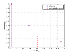
Figure 4: Channel estimation with $p=5$ sampling channels, and SNR=$15$dB.

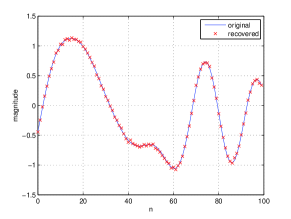
Figure 5: Estimation of the time-varying gain coefficient of the first path, $p=5$, SNR=$15$dB.

VII-B Performance in the presence of noise

In the next simulations we examine the effect of SNR and the number of sampling channels on the error in the delays estimation. We choose $K=2$ close delays, $t_{1}=0.4352T$ and $t_{2}=0.521T$. The sequences $a_{k}[n],k=1,2,\,n=1,2,\ldots 100$ are finite length sequences with unit power chosen according to Jakes’ model with $f_{d}=0.05/T$.

Under the setting of the simulation, which consists of a pulse with constant frequency response and ideal band-pass filters, from (23) it can be verified that the sampling sequences satisfy the following relation in the time domain

$$\mathbf{c}\left[n\right]=\mathbf{N}\left(\tau\right)\mathbf{b}\left[n\right],\quad n\in\mathbb{Z}.$$ (72)

The Cramer-Rao bound (CRB) for unbiased estimators of $\theta_{k}=\frac{2\pi}{T}t_{k}$ from the data $\mathbf{c}\left[n\right]$, was derived in [43] for this data model. The TLS-ESPRIT algorithm, used for the delays estimation in our method, is known to be asymptotically unbiased [44]. Experimentally we verified that, under the simulation setup, the bias of the delays estimation is low enough for SNRs above $15$dB. Therefore, in this range of SNRs, the CRB derived in [43] can give a lower bound on the MSE of the delays estimation (up to factor of $\frac{2\pi}{T}$), assuming our specific sampling scheme.

In Fig. 6, the mean-squared error (MSE) of the time delays estimation is shown versus the SNR, when using $p=4$ sampling channels. For comparison we also plot the CRB. The figure demonstrates that our method achieves the CRB for SNR$>15$dB, which is the range that delays estimation can be considered as unbiased.

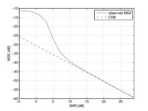
Figure 6: MSE of the delays estimation versus SNR, for $K=2$ and $p=4$.

In Fig. 7, the MSE of the estimation of the time delays is shown versus the number of sampling channels, for a constant SNR of $10$dB. The results demonstrate that the estimation error can be improved by increasing the number of channels. Therefore, oversampling improves the robustness of our method to noise.

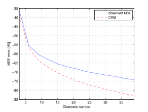
Figure 7: MSE of the delays estimation versus the number of sampling channels $p$, for $K=2$ and SNR=$10$dB.

VII-C Effects of imperfect approximation of $\mathbf{R}_{dd}$

Next, we investigate the influence of estimating the matrix $\mathbf{R}_{dd}$ using only a finite number of measurement vectors $\mathbf{d}\left[n\right]$. This number effects the total delay of our method, since reconstruction of the sequences $a_{k}\left[n\right]$ is performed only after the unknown delays $\tau$ are recovered. In Fig. 8 the MSE of the delays estimation is shown versus the number of measurement vectors used for estimation of $\mathbf{R}_{dd}$. A constant SNR of $20$dB and $p=4$ sampling channels are used. Two cases are illustrated: in the first, the sequences $a_{k}\left[n\right]$ are taken according to the Jakes’ model with parameter $f_{d}=0.05/T$ and in the second case $f_{d}=0.1/T$ is used, which corresponds to sequences with faster variation rate. Fig. 8 demonstrates that the MSE depends on the variation rate of the sequences. Intuitively the faster the sequences vary, the more information each new measurement vector $\mathbf{d}\left[n\right]$ contains, improving the estimation of $\mathbf{R}_{dd}$. In addition, it can be seen that using only $50$ measurement vectors, yields a reasonable estimation of the delays in the case of $f_{d}=0.1/T$. The same estimation error is achieved using $80$ measurement vectors, when using slow varying sequences. This result can be further improved by increasing the SNR or the number of sampling channels.

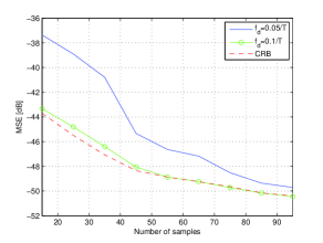
Figure 8: MSE of the delays estimation versus the number of samples used, for $K=2$, $p=4$ and SNR=$20$dB.

VII-D Effects of imperfect digital filtering correction

In the next simulation we examine the effects of approximating the digital correction filter bank $\mathbf{W}^{-1}\left(e^{j\omega T}\right)$ by finite length digital filters. The length of the filters affects the delay of our scheme. To demonstrate this point, we arbitrarily choose a sampling scheme composed of $3$ non ideal band-pass filters with a frequency response given by

$$S_{\ell}\left(\omega\right)=\begin{cases}1.1-\left(1-0.4\ell\right)\textrm{cos}\left(\omega-\frac{2\pi}{T}\ell\right)&\omega\in\mathcal{F}_{\ell}\\ 0&\textrm{otherwise},\end{cases}$$ (73)

where

$$\mathcal{F}_{\ell}=\left[\left(\ell-1\right)\frac{2\pi}{T},\ell\frac{2\pi}{T}\right].$$ (74)

These filters satisfy the conditions of Proposition 1 and can model realistic sampling filters with non-flat frequency response. In this case a non trivial digital correction filter bank is required, whose coefficients are calculated using the inverse DTFT of $\mathbf{W}^{-1}\left(e^{j\omega T}\right)$.

In Fig. 9 the MSE of the delays estimation versus the SNR is plotted for different lengths of filters. At low SNRs the dominant error is caused by the noise, while for high SNRs the error is mostly a result of the correction filter approximation. It can be seen that a $49$ taps filters provide a good approximation to the correction filter bank, resulting in a delay of $24$ samples. When working at SNRs below $40$dB, filters with $11$ taps provide a reasonable approximation.

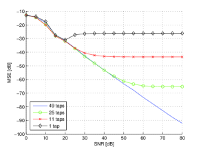
Figure 9: MSE of the delays estimation versus SNR for different lengths of digital correction filter bank approximations.

VIII Conclusion

In this paper, we considered the problem of estimating the time delays and time varying coefficients of a multipath channel, from low-rate samples of the received signal. We showed that this problem can be formulated within the broader context of sampling theory, in which our goal is to recover an analog signal $x(t)$ that lies in a SI subspace, spanned by $K$ generators with unknown delays. This class of problems can be viewed as an infinite union of subspaces.

We showed that if the channel has $K$ multipath components, or equivalently, if the SI subspace is generated by $K$ generators, than under appropriate conditions on the sampling filters, a sampling rate of $2K/T$ is necessary and sufficient to guarantee perfect recovery of any signal $x(t)$. Here $T$ is the transmission rate, or the period of the generators. We developed sufficient conditions on the generators and the sampling filters in order to guarantee perfect recovery at the minimal possible rate. To recover the unknown time delays, we showed that our problem can be formulated within the context of DOA estimation. Using this relationship, we proposed an ESPRIT-type algorithm to determine the unknown delays from the given low rate samples. Once the delays are properly identified, the time varying coefficients can be found by digital filtering.

Besides the application to time delay estimation, the problem we treated here can be seen as a first example of a systematic sampling theory for analog signals defined over an infinite union of subspaces. Recently, there has been growing interest in sampling theorems for signals over a union of subspaces [15, 16, 20, 18, 19, 17, 22]. However, previous work addressing stability issues and concrete recovery algorithms have focused on finite unions. Here, we take a first step in the direction of extending these ideas to a broader setting that treats analog signals lying in an infinite union.

References

- [1] A. Quazi, “An overview on the time delay estimate in active and passive systems for target localization,” IEEE Trans. on Acoustics, Speech and Signal Processing, vol. 29, no. 3, pp. 527–533, 1981.
- [2] R. J. Urick, Principles of Underwater Sound. McGraw-Hill New York, 1983.
- [3] G. L. Turin, “Introduction to spread-spectrum antimultipath techniques and their application to urban digital radio,” Proceedings of the IEEE, vol. 68, no. 3, pp. 328–353, March 1980.
- [4] A. Bruckstein, T. J. Shan, and T. Kailath, “The resolution of overlapping echos,” IEEE Trans. on Acoustics, Speech and Signal Processing, vol. 33, no. 6, pp. 1357–1367, 1985.
- [5] M. A. Pallas and G. Jourdain, “Active high resolution time delay estimation for large BT signals,” IEEE Trans. on Signal Processing, vol. 39, no. 4, pp. 781–788, Apr 1991.
- [6] R. Schmidt, “Multiple emitter location and signal parameter estimation,” IEEE Trans. on Antennas and Propagation, vol. 34, no. 3, pp. 276–280, Mar 1986.
- [7] Z. Q. Hou and Z. D. Wu, “A new method for high resolution estimation of time delay,” IEEE International Conference on Acoustics, Speech, and Signal Processing, ICASSP ’82, vol. 7, pp. 420–423, May 1982.
- [8] H. Saarnisaari, “TLS-ESPRIT in a time delay estimation,” IEEE 47th Vehicular Technology Conference, 1997, vol. 3, pp. 1619–1623 vol.3, May 1997.
- [9] F.-X. Ge, D. Shen, Y. Peng, and V. O. K. Li, “Super-resolution time delay estimation in multipath environments,” IEEE Trans. on Circuits and Systems, vol. 54, no. 9, pp. 1977–1986, Sept. 2007.
- [10] R. Kumaresan and D. W. Tufts, “Estimating the angles of arrival of multiple plane waves,” IEEE Trans. on Aerospace and Electronic Systems, vol. AES-19, no. 1, pp. 134–139, Jan. 1983.
- [11] R. Roy and T. Kailath, “ESPRIT-estimation of signal parameters via rotational invariance techniques,” IEEE Trans. on Acoustics, Speech and Signal Processing, vol. 37, no. 7, pp. 984–995, Jul 1989.
- [12] Y. C. Eldar and T. Michaeli, “Beyond bandlimited sampling,” IEEE Signal Processing Magazine, vol. 26, no. 3, pp. 48–68, May 2009.
- [13] D. H. Johnson and D. E. Dudgeon, Array signal processing : concepts and techniques. Englewood Cliffs, NJ: Prentice-Hall, 1993.
- [14] H. Krim and M. Viberg, “Two decades of array signal processing research: the parametric approach,” IEEE Signal Processing Magazine, vol. 13, no. 4, pp. 67–94, Jul 1996.
- [15] Y. M. Lu and M. N. Do, “A theory for sampling signals from a union of subspaces,” IEEE Trans. on Signal Processing, vol. 56, no. 6, pp. 2334–2345, June 2008.
- [16] T. Blumensath and M. E. Davies, “Sampling theorems for signals from the union of finite-dimensional linear subspaces,” IEEE Trans. on Inform. Theory, vol. 55, pp. 1872–1882, April 2009.
- [17] Y. C. Eldar, “Compressed sensing of analog signals in shift-invariant spaces,” IEEE Trans. on Signal Processing, vol. 57, no. 8, pp. 2986–2997, Aug. 2009.
- [18] M. Mishali and Y. C. Eldar, “Blind multiband signal reconstruction: Compressed sensing for analog signals,” IEEE Trans. Signal Processing, vol. 57, pp. 993–1009, Mar. 2009.
- [19] ——, “From theory to practice: Sub-Nyquist sampling of sparse wideband analog signals,” submitted to IEEE Selected Topics on Signal Processing.
- [20] Y. C. Eldar and M. Mishali, “Robust recovery of signals from a structured union of subspaces,” to appear in IEEE Trans. on Inform. Theory.
- [21] M. Mishali and Y. C. Eldar, “Reduce and boost: Recovering arbitrary sets of jointly sparse vectors,” IEEE Trans. on Signal Processing, vol. 56, no. 10, pp. 4692–4702, Oct. 2008.
- [22] Y. C. Eldar, “Uncertainty relations for analog signals,” to appear in IEEE Trans. on Inform. Theory.
- [23] M. Vetterli, P. Marziliano, and T. Blu, “Sampling signals with finite rate of innovation,” IEEE Trans. on Signal Processing, vol. 50, no. 6, pp. 1417–1428, Jun 2002.
- [24] P. L. Dragotti, M. Vetterli, and T. Blu, “Sampling moments and reconstructing signals of finite rate of innovation: Shannon meets strang-fix,” IEEE Trans. on Signal Processing, vol. 55, no. 5, pp. 1741–1757, May 2007.
- [25] A. Aldroubi and K. Gröchenig, “Non-uniform sampling and reconstruction in shift-invariant spaces,” Siam Review, vol. 43, pp. 585–620, 2001.
- [26] C. de Boor, R. A. DeVore, and A. Ron, “The structure of finitely generated shift-invariant spaces in ,” Journal of Functional Analysis, vol. 119, no. 1, pp. 37–78, 1994.
- [27] J. S. Geronimo, D. P. Hardin, and P. R. Massopust, “Fractal functions and wavelet expansions based on several scaling functions,” Journal of Approximation Theory, vol. 78, no. 3, pp. 373–401, 1994.
- [28] O. Christensen and Y. C. Eldar, “Generalized shift-invariant systems and frames for subspaces,” Journal of Fourier Analysis and Applications, vol. 11, no. 3, 2005.
- [29] P. Stoica and R. Moses, Introduction to spectral analysis. Englewood Cliffs, NJ: Prentice-Hall, 1997.
- [30] E. Moulines, P. Duhamel, J. Cardoso, S. Mayrargue, and T. Paris, “Subspace methods for the blind identification of multichannel fir filters,” IEEE Trans. on Signal Processing, vol. 43, no. 2, pp. 516–525, 1995.
- [31] M. Wax and I. Ziskind, “On unique localization of multiple sources by passive sensor arrays,” IEEE Trans. on Acoustics, Speech and Signal Processing, vol. 37, no. 7, pp. 996–1000, Jul 1989.
- [32] M. Z. Win and R. A. Scholtz, “Characterization of ultra-wide bandwidth wireless indoor channels: A communication-theoretic view,” IEEE Journal on Selected Areas in Communications, vol. 20, no. 9, pp. 1613–1627, Dec 2002.
- [33] B. Le, T. W. Rondeau, J. H. Reed, and C. W. Bostian, “Analog-to-digital converters,” IEEE Signal Processing Magazine, vol. 22, no. 6, pp. 69–77, Nov. 2005.
- [34] J. E. Evans, D. F. Sun, and J. R. Johnson, “Application of advanced signal processing techniques to angle of arrival estimation in ATC navigation and surveillance systems,” MIT, Lincoln Lab. Tech. Rep, 1982.
- [35] T.-J. Shan, M. Wax, and T. Kailath, “On spatial smoothing for direction-of-arrival estimation of coherent signals,” IEEE Trans. on Acoustics, Speech and Signal Processing, vol. 33, no. 4, pp. 806–811, Aug 1985.
- [36] D. L. Donoho, “Compressed sensing,” IEEE Trans. on Inform. Theory, vol. 52, no. 4, pp. 1289–1306, 2006.
- [37] H. Meyr, M. Moeneclaey, and S. A. Fechtel, Digital communication receivers: synchronization, channel estimation, and signal processing. Wiley, New York, 1997.
- [38] J. G. Proakis, Digital communications, 3rd ed. McGraw-Hill, New York, 1995.
- [39] S. E. Bensley and B. Aazhang, “Subspace-based channel estimation for code division multiple access communication systems,” IEEE Trans. on Communications, vol. 44, no. 8, pp. 1009–1020, 1996.
- [40] E. G. Strom, S. Parkvall, S. L. Miller, and B. E. Ottersten, “DS-CDMA synchronization in time-varying fading channels,” IEEE Journal on Selected Areas in Communications, vol. 14, no. 8, pp. 1636–1642, Oct 1996.
- [41] L. Yang and G. B. Giannakis, “Ultra-wideband communications: An idea whose time has come,” IEEE Signal Processing Magazine, vol. 21, no. 6, pp. 26–54, 2004.
- [42] W. C. Jakes, Microwave mobile communications. Wiley, New York, 1974.
- [43] P. Stoica and N. A., “Music, maximum likelihood, and Cramer-Rao bound,” IEEE Trans. on Acoustics, Speech and Signal Processing, vol. 37, no. 5, pp. 720–741, May 1989.
- [44] B. Ottersten, M. Viberg, and T. Kailath, “Performance analysis of the total least squares ESPRIT algorithm,” IEEE Trans. on Signal Processing, vol. 39, pp. 1122–1135, May 1991.