Multilevel Coding over Two-Hop Single-User Networks
Abstract
In this paper, a two-hop network in which information is transmitted from a source via a relay to a destination is considered. It is assumed that the channels are static fading with additive white Gaussian noise. All nodes are equipped with a single antenna and the Channel State Information (CSI) of each hop is not available at the corresponding transmitter. The relay is assumed to be simple, i.e., not capable of data buffering over multiple coding blocks, water-filling over time, or rescheduling. A commonly used design criterion in such configurations is the maximization of the average received rate at the destination. We show that using a continuum of multilevel codes at both the source and the relay, in conjunction with decode and forward strategy at the relay, performs optimum in this setup. In addition, we present a scheme to optimally allocate the available source and relay powers to different levels of their corresponding codes. The performance of this scheme is evaluated assuming Rayleigh fading and compared with the previously known strategies.
I Introduction
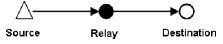
In recent years, relay-assisted transmission has gained significant attention as a powerful technique to enhance the performance of wireless networks. The main idea is to employ some extra nodes (relay nodes) in the network to facilitate the communication between the terminal nodes. The concept of relaying was first introduced by Van der Meulen in [1] and is defined as a scheme to improve the coverage/reliability of a wireless network. For instance, relays are usually deployed in networks when the direct link between the source and the destination is either blocked or has a very poor quality. The term two-hop network usually refers to such a network configuration in which there is no direct link between the source and the destination, and one relay node assists the transmission of data between the end terminals, see Fig. 1. Two-hop networks have been implemented widely in different applications, including TV broadcasting and satellite communications.
Following the introduction of relay channel in [1], Cover and El Gamal introduce two different coding strategies for single relay networks [2]. In the first strategy, known as “Decode and Forward” (), the relay decodes the transmitted message and cooperates with the source to send the message in the next block. Instead of decoding, in the second strategy, the relay compresses the received signal and forwards it to the destination in the next block. The terms “Compress and Froward” () or “Quantize and Forward” () usually refer to this transmission scheme. Besides and , in some recent results, [3, 4, 5, 6], the authors investigate another transmission scheme called “Amplify and Forward” () for the Gaussian relay network. In this strategy, without decoding the information, the relay amplifies the received signal and retransmits it to the destination.
Knowing these schemes, the performance of relaying is analyzed for different network topologies. For instance, considering a single-relay network, authors of [5] and [6] derive a single-letter expression for the maximum achievable rate of relaying using a simple linear scheme (assuming frequency division and AWGN channel). As another example, [4] shows that relaying achieves the network capacity of Gaussian parallel single-antenna relay network. The extension of [4] to the case of multiple-antenna Rayleigh fading networks is presented in [7] and [8]. The first capacity result for relay networks is obtained in [2], where the authors prove the optimality of strategy in a single-relay network when the received signal at the destination is a degraded version of the relay received signal. Clearly, the degradedness condition holds in the two-hop setting. Thus, would be the optimal relaying scheme for two-hop networks. Indeed, most of the results in the literature on relay networks either assume static channels between the nodes or perfect knowledge of the Channel State Information (CSI) at both end nodes of each link, for the case of fading channels.
Recently, some papers discuss different transmission schemes over relay networks when the CSI is not available at the transmitting nodes, where most of them focus on Diversity-Multiplexing Trade-off (DMT) [9, 10, 11, 12, 13, 14]. Obviously, for such settings, the ergodic capacity is not defined, however, the outage capacity is defined as the maximum rate decodable with a given probability [15]. From the throughput maximization point of view, the goal is to propose a scheme to maximize the average data rate received at the destination. The simplest form of such a problem is to find the optimal transmission strategy for a one-hop single-user network when CSI is available only at the receiver and the channel has quasi-static fading characteristic. In a pioneering work, Shamai has addressed this problem by substituting the receiver by a continuum of virtual receivers, each corresponding to a specific realization of the channel gain [16]. Relying on the resulting degraded broadcast channel, [16] shows that an infinite-level coding scheme with a proper power allocation among the different levels of code maximizes the destination’s average data rate.
There are several extension for this work; in [17, 18, 19] the authors try to find the optimal transmission strategy when partial information is available at the source. [20] suggests the application of multilevel coding in a multicast network with some QoS constraints and derives the optimum throughput-coverage trade-off for such a network. [21] combines multilevel coding scheme with Hybrid Automatic Retransmission Request (HARQ) and shows that this approach results in high throughput and low latency in a point-to-point link. The Multiple Input Multiple Output (MIMO) extension of [16] is also discussed in [22], [23], and [24].
Considering the two-hop network with no CSI at the transmitter side of each link, Steiner et al in [25] propose different transmission schemes, assuming that the relay node has a power constraint and is simple, i.e., is not capable of data buffering over multiple coding blocks or rescheduling. To find the optimal transmission scheme, they study different multilevel coding schemes when the relay operates in different modes, including , , and . As discussed in [25], due to the high complexity of the infinite-level coding scheme, they have only considered a finite level code in their proposed strategies. Comparing the results of [25], it turn out that strategy outperforms all other investigated transmission schemes, specifically in the high SNR regime. However, as concluded in [25], although has the best performance among the other strategies, the optimality of scheme is not implied. In fact, since the general infinite-level coding scheme remains unsolved, there is always a question of whether or not relaying achieves a higher expected rate as compared to . The main motivation of this work is to answer this question.
In this work, we study the performance of relaying scheme which uses infinite-level codes at the source and the relay in the same setup as in [25]. To this end, we first prove that the infinite-level code and relaying is indeed the optimal two-hop transmission strategy for maximizing the destination’s average data rate. We further propose an algorithm to determine the optimum power allocation for each indefinite-level code. Numerical results are presented to verify that the proposed scheme outperforms the strategy discussed in [25].
The organization of this paper is as follows: First, section II describes the two-hop system model. A brief review of some previous results on single-hop links are presented in section III. Formulating the multilevel coding scheme in subsection IV-A, we prove the optimality of this scheme in subsection IV-B. Afterwards, in section IV-C, we present a procedure to actually determine the optimal infinite-level code parameters at the source and the relay. Numerical results and comparison with other schemes for the special case where both links are Rayleigh fading is presented in section V. Finally, section VI concludes the paper.
Throughout this paper, we represent the expectation operation by . The notation is used for the natural logarithm and rates are expressed in nats. We denote and as the probability density function (pdf) and the cumulative distribution function (CDF) of random variable .
II System Model
In this paper, we investigate the performance of a two-hop network, in which a relay assists the transmission of data between a source and a destination. As Fig. 1 shows, in a two-hop network, the destination can solely receive data via the relay. All nodes are assumed to have single antennas.
It is assumed that the source has no information about either of the channel gains, the relay knows only the channel gain between itself and the source, and the destination knows both channel gains. This CSI assumptions are indeed practical, since the receiver of each hop can evaluate its immediate channel gain by measuring the pilot signal sent from the corresponding transmitter. In addition, the receiver can measure the equivalent channel (the source to the destination) if the relay forwards the pilot signal of the source towards the destination. Having the equivalent channel gain and the relay to destination channel gain, the destination can find the source to relay channel gain as well.
It is also assumed that the source and relay both know the fading power distribution of both links. By and we denote the probability density function of fading power in the first and second hop, respectively. The channels of both links are assumed to be quasi-static, i.e., they are chosen randomly (based on their corresponding pdf) at the start of the transmission and remain fixed for the whole transmission.
Source and relay are assumed to have power constraints and , respectively. Furthermore, they are assumed to be capable of constructing infinite-level codes. However, the relay is assumed to be simple, i.e., is not capable of buffering any unsent data, rescheduling the untransmitted data from the previous blocks. It is also assumed that the relay can not perform water-filling of its power over multiple blocks and has a maximum power constraint in each block. Therefore, it can only retransmit the data which it has just received from the first hop. Successive decoding is used as the decoding procedure at both destination and relay (in case the relay wants to decode the data).
III Multilevel Coding Scheme for Single-hop Networks
In this section, we review some previous studies on the application of the multilevel codes for a single-hop network in two scenarios: 1) No CSI is available at the transmitter, which is known as “broadcasting approach” [16] and 2) no CSI is available at the transmitter and in addition, the transmission data rate can not exceed a certain value [25].
III-A Single-Hop Broadcasting Strategy
The optimum scheme for a single-hop link, in case that the transmitter knows the fading power for each block is to design a single-level code with the rate of for that block. Here, denotes the normalized transmission power, i.e, the equivalent transmission power if the noise power is equal to one and is the fading power for that specific block. Therefore, the average achievable rate for this setup would be [26].
Although designing a single-level code is optimum in the above scenario, it can not be applied for a transmitter which does not have access to the channel state information. For such a scenario, Shamai has introduced a technique called broadcasting strategy [16]. In this technique, the transmitter sends the data through infinite levels of a superposition code. Then, conditioned on the channel state, i.e., the fading power, the receiver decodes up to a certain level of the code. Therefore, the total receiving rate for each channel realization, say , can be evaluated as:
| (1) |
where represents the differential rate transmitted over level ‘’ of the code. Defining as the power assigned for the level, is given by:
| (2) | |||||
where and the second line follows from the assumption of infinitesimal rate assignment which is shown to be optimal in [20] . The aim is to find a such that the average data rate at the destination is maximized while the source power constraint () holds. It means that the power should be assigned to different code levels such that:
| (3) | |||||
where shows the pdf of the channel fading power.
This maximization problem has been studied and solved using calculus of variations technique (see [16] for details of the proof). Here, we only mention the final solution as:
| (7) |
where is the CDF of the fading power. and are determined such that they satisfy and , respectively. Clearly, the optimum power assignment can be determined by . The maximum destination’s average data rate will be:
| (8) |
where is obtained by setting in (1) and (2). The total rate of the final superimposed code can be evaluated by:
| (9) |
Note that this value only depends on the fading power distribution and the transmitter power.
Finally, it is important to mention that the above scheme is indeed the optimal transmission scheme for a fading link when the source does not have the CSI. It is due to the result of [27] which proves that the multilevel coding maximizes any weighted sum-rate of a degraded broadcast channel. Therefore, considering the equivalent broadcast model for the single-user fading channel, the multilevel coding achieves the optimal destination’s average data rate.
III-B Single-Hop Rate-Limited Broadcast Strategy
An interesting extension of the above broadcast strategy is designing a multilevel code for a source with available data rate limited to , i.e., the transmission rate should be less than [25].
The problem formulation is similar to subsection III-A, except it has one more constraint on the transmission rate. The modified optimization problem will be, [25]:
| (10) | |||||
where the second condition ensures that the transmission rate remains less than the available source data rate.
Reference [25] uses constrained calculus of variations to solve this problem. More precisely, initially the authors in [25] substitute the first constraint by two end-point conditions of and . Then, using and Lagrangian multiplier, (10) is reconstituted as a variations problem (See [25] for more details). It turns out that the optimum distribution function is as follows:
| (14) |
where . and are determined as a function of and satisfy and , respectively. Finally, is computed such that the transmission rate constraint holds.
As an example, for the case of Rayleigh fading channel, i.e., , the optimum distribution is as follows [25]:
| (18) | |||||
| (19) |
where is the Lambert W-function and finds such that . The values for and are also determined by solving the following system of equations:
| (22) |
One important observation is that in the case of ( is defined in equation (9)) the above rate-limited problem will be simplified to the original problem in subsection III-A. Although this statement can be verified mathematically, its intuitive explanation would be insightful. It is obvious that if tends to infinity, the rate condition is always satisfied (will not be an active constraint). Therefore, maximization problem of (10) relaxes to the form of equation (3). Moreover, III-A shows that the source, in the optimal transmission of the original problem (without rate constraint), feeds the channel with a rate equal to . Hence, it turns out that even though the available rate at the source is more than , the source needs to transmit only bits of information in each block. Therefore, if , the solutions of the two optimization problems of (3) and (10) are equal.
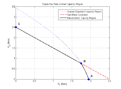
At the end, note that the resulted multilevel code is also the optimal transmission scheme for the rate-limited one-hop set-up. To prove, we should use the broadcast equivalent structure of the network. Indeed, the capacity region of the rate-limited degraded broadcast network is the intersection of the original degraded broadcast channel capacity region and the region below the surface associated with the transmission rate constraint. For illustration, the solid line in Fig. 2 shows a typical capacity region of a rate-limited two-user degraded broadcast channel. In this figure, dotted and dashed lines depict the capacity region of the original degraded broadcast channel (without rate limitation) and the line representing the rate constraint, respectively. The destination’s average data rate can be evaluated as the sum of the received data rate for each channel state () times the probability of occurring that specific channel state (). Clearly, this value is maximized on the boundary of the resulted capacity region (the solid line). Therefore, the optimal point would be either over the capacity region without rate limitation (Arc ) or the end point of the rate limitation line (Point C). Since is a part of the original capacity region, multilevel coding is the optimal scheme to achieve any point on . Furthermore, point C is archived using a single level code which is again a special case of multilevel codes. This proves the optimality of multilevel coding scheme for rate limited scenarios.
IV Multilevel Coding Scheme for Two-hop Networks
As an extension of the one-hop set-up, [25] addresses the problem of maximizing the destination’s average data rate in a two-hop network, where there is no direct link between the source and the destination. In reference [25], several schemes have been studied, including broadcasting strategy with relaying, and relaying with finite level broadcasting at the source and the relay. Infinite level codes with relaying is also addressed in [25]. However, the performance of this method remains as an open problem there.
In this section, we will first describe the infinite level strategy in details. Then, in subsection IV-B, we prove the optimality of this scheme. Finally, subsection IV-C presents an algorithm to optimally design such an infinite level code.
IV-A Infinite-Level Codes for Two-hop Networks
Based on the system model, each transmission block of the infinite level strategy consists of the following two steps:
-
1.
In the first phase, the source allocates its power among different code levels with the power distribution function . Of course, should satisfy the power constraint . Then, based on the source-relay channel fading power, say , the relay is able to decode up to the level of the transmitted data. Thus, the relay received rate is:
(23) where .
-
2.
In the second phase, the relay should transmit the data to the destination. As noted earlier, in this work, we only focus on simple relays which can neither buffer any of the previously received data nor do any scheduling tasks. As a results, these relays have two features which seem obvious but have important effects on the code design. To illustrate, consider a case in which the relay has decoded bits of the transmitted data. It turns out that, firstly, the relay can not transmit with the rate greater than . Secondly, if the relay transmits with the rate , , the rest of the data () can not be stored and should be discarded. Consequently, the relay, in each transmission block, should choose the optimal power distribution of the multilevel code such that it satisfies the relay total power constraint (). Meanwhile, the relay should keep the transmission rate below its received data rate in that block ().
Defining as the power distribution of each code level at the relay conditioned on the input rate of , we can summarize these conditions as:
-
(a)
Power constraint at the relay:
. -
(b)
Available rate constraint at the relay:
, where is defined by (23).
Clearly, the relay requires to know for all possible values of .
Transmitting a multilevel code on the relay-destination link, the destination is able to decode up to a certain level ‘’. Here, ‘’ denotes the fading power of the second link. Therefore, for each , the received data rate at the destination can be written as:
(24) Indeed, for successful decoding of the signal, the destination should know the power allocation strategy of the relay. This information can be obtained through the knowledge of the source to the relay channel gain.
-
(a)
Given these, we are now able to formulate the two-hop optimization problem. Similar to the single-hop scenario, we want to maximize the average data rate received at the destination. Assuming and as the probability density functions of the fading power in the source-relay and relay-destination links, respectively, the destination’s average data rate can be written as:
Therefore, we obtain the final optimization problem as follows:
| (26) | |||||
Note that the above optimization problem is similar to the one derived in [25]. However, in [25], the last constraint (relay rate limitation) is stated as an equality. In fact, it is more accurate to formulate the rate limitation by an inequality constraint instead of equality. It is due to the fact that the relay may not have to send all information it receives from the first hop to achieve the optimal performance. In other words, the last constraint of equation (26) lets the relay to discard some of its received data if it wants to do so. For instance, this may happen when the relay receives data rate higher than its corresponding ( is defined in equation (9)). In such a scenario, the relay only uses bits of the received information and ignores the rest.
IV-B Optimality of Two-Hop Multilevel Coding
The main focus of this section is to show that the multilevel coding approach combined with decode and forward () relaying maximizes the average data rate at the destination of a two-hop network.
To start, let us emphasize that according to the two-hop structure of the network, all information received by the destination should be first passed through the relay and there is not any direct link between the source and the destination. As a result, the destination received signal is always a degraded version of what has been received at the relay. In other words, no information can be decoded by the destination unless it has been decodable at the relay. Thus, it can be concluded that decode and forward is the optimal relaying scheme for two-hop settings.
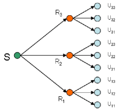
Knowing the optimality of , similar to the single-hop network (See [22]), we model both first and second fading hops by infinite number of virtual relays and virtual users, respectively. More precisely, we substitute the relay with infinite relays, each has a constant channel gain which corresponds to a specific realization of the first hop channel. These virtual relays constitute a degraded set. If we assume that the channel fading power is selected from a set of discrete values 111Note that here, for simplicity, we assume that the fading levels of both links are selected from the same set. However, the statements of optimality holds for the general case. Moreover, this assumption is valid for the case of , there would be virtual relays in the network. Without loss of generality, we assume . Of course, this model is accurate only if tends to infinity. In a similar way, the second hop can be modeled with virtual users for each of the virtual relays; thus, in total there would be virtual users in the network. denotes the virtual user which is associated to the virtual relay , and its channel gain is . Moreover, represents the decodable rate at this node. For illustration purpose, Fig. 3 depicts the network model for the case that , i.e., .
The aim is to find the optimum transmission scheme for the source and the relay. We start from the second hop and assume the source uses an arbitrary transmission scheme. Furthermore, let be the rate that each of the virtual relays, i.e., , can decode under this transmission scheme. Having the data rate at relay , the optimal second-hop strategy is to maximize the destination’s average data rate for each of the virtual relays. As will be described in subsection IV-C, the solution to this problem is similar to the result of the subsection III-B and the optimal power distribution, , for each of the virtual relays can be determined by (14), in which . In other words, multilevel coding is the optimal strategy for the second hop.
Note that the successful decoding is only possible if the destination knows the applied (or equivalently the value of ) at the relay. In our two hop model, this information can be obtained by the knowledge of the source to the relay channel gain at the destination. The optimal received data rate for each of the virtual users, say , can be evaluated by:
| (27) |
where . Let be probability that the second hop gain is equal to . Hence, the optimal average rate of the second hop under rate condition would be:
| (28) |
Given , the two-hop network average data rate can be written as:
| (29) |
where represents the probability that the first hop channel is in state . The goal of the code design is to maximize . As (29) shows, the destination’s average data rate is the weighted sum of a non-linear function of . The domain of acceptable for is a convex set which is known as the capacity region of the underlying broadcast channel. Moreover, due to the degradedness of the virtual relays, all points on the boundary of this capacity region can be achieved by a multilevel code [2]. Therefore, to prove the optimality of the multilevel code for the first hop, it is enough to show that is maximized on the boundary of this capacity region. This argument can also be justified if we can show that is positive . To show this, we write:
| (30) |
where is defined in equation (28) and shows the destination’s average data rate when the relay has the rate constraint of . By definition, is a non-negative value. Moreover, from the results of subsection III-B, it can be concluded that is non-negative. In fact, if , where is defined in equation (9), then and , otherwise. Therefore, for . Consequently, is maximized for the values of which are on the boundary of the capacity region of the first hop broadcast channel. In other words, the multilevel coding scheme is the optimal transmission strategy for the first hop. This completes the proof for the optimality of multilevel coding for the two-hop network.
IV-C Optimal Design of Two-Hop Multilevel Coding
Having the optimality of two-hop multilevel coding scheme, in this section, we present a procedure in order to solve the two-hop optimization problem introduced in equation (26). The main difficulty of this problem is that, unlike single-hop scenarios (the original and the rate-limited broadcasting cases), equation (26) can not be directly solved by variations methods. It is due to the fact that the constraint on the second hop rate does not have a fixed value on the right hand side, i.e., it does not have a form of isoperimetric problem. For a complete discussion on isoperimetric problem, refer to [28]. To solve this problem, we use the following lemma.
Lemma IV.1
The following maximization problems on two non-negative functions and :
| (31) |
and
| (32) |
where and are two known non-negative functions, are equivalent.
Proof:
Using this lemma and noting that , we can reform in (26) as follows:
| (35) | |||||
where the outer maximization is subject to:
| (36) |
and the constraints of the inner problem are as follows:
| (37) | |||
| (38) |
In (35), follows from the fact that can be determined with the knowledge of and and the dependence of the term on is only through .
Given (35)-(38), in the following two subsections, we will discuss how this two-step maximization problem can be solved using Euler’s equations [29].
IV-C1 Relay-Destination Link Optimization Problem
Receiving bits from the first hop, the aim of the relay is to maximize the average data rate received at the destination. In fact, if the input rate changes, the relay should modify its power distribution, accordingly. However, the knowledge of the input rate (), the relay total power, and the pdf of the second hop fading power is sufficient for determining the optimum power distribution function, . It is evident that the optimum power distribution function, , can be completely determined by evaluating for all values of . , itself, is the solution of the following problem:
Note that, in (IV-C1), is a constant; hence, the problem takes the form of the rate-limited broadcast strategy problem, subsection III-B. Therefore, the optimum solution is:
| (43) |
where . and are determined as a function of to satisfy and , respectively. The optimum multilevel power distribution at the relay can be found by . Finally, is computed to satisfy:
| (44) |
where is defined by (9). This condition comes from the fact that achieving the maximum average rate at the destination requires the relay not to transmit more than bits (refer to the discussion in subsection III-B).
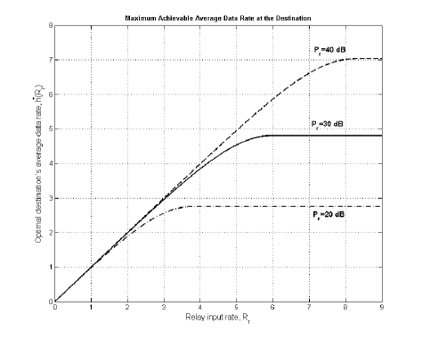
As an example, we have solved (IV-C1) for a network in which the second hop can be modeled as a Rayleigh fading channel, i.e., . Fig. 4 shows the maximum destination’s average data rate, , for different relay input rates () and different relay powers ().
IV-C2 Source-Relay Link Optimization Problem
Knowing the optimum value for the inner integration, , (35) can be written as follows:
| (45) | |||||
where:
| (49) |
and . and satisfy and , respectively. As (49) suggests, only depends on , , and . Remembering , we can write the integrand of (45) as . With this notation, equation (45) takes the form of a fixed end-point Calculus of Variations problem and can be solved using Euler’s equation, [29],
| (50) |
where , , and is the derivative of with respect to . Thus, we have:
| (53) |
| (56) | |||||
| (62) |
where and denote the first order and the second order derivative of , respectively. Substituting (53)-(62) in (50), the optimal is derived.
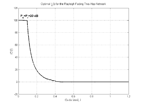
As an example, in the scenario where both source-relay and relay-destination links are modeled with a Rayleigh fading channel, i.e., , (50) can be simplified to:
where . To solve (IV-C2), we first need to have and . Indeed, these functions can be numerically evaluated using the results of subsection IV-C1. In the next step, we replace by , corresponding to the amount of interference in each level222In fact, we have approximated a continuous variable with a discrete -level function, which becomes precise as tends to infinity.. ’s are in descending order, such that and . As a result, we have a nonlinear system of equations, i.e., which can be solved numerically. The final solution for these variables shows the optimal interference function, . As an example, Fig. 5 presents in the case of Rayleigh fading model for both hops and dB. Having , the amount of power associated for each code level can be determined by .
V Numerical Results and Comparison with Other Schemes
In the previous sections, we have proposed a multilevel coding scheme, which is shown to be optimum in the underlying network setup, and derived the optimum source and relay power distribution through different levels of code. In this section, we compare the performance of the proposed scheme (which is the optimal scheme) with the cut-set upper-bound and two other sub-optimal schemes proposed in [25].
-
A.
Broadcasting Cutset Bound, :
This bound simply says that the achievable average data rate of a two-hop network can not exceed the achievable average rate of any of the single-hop links, i.e., the source-relay and the relay-destination links. This is independent of the relay structure and its operation. In other words, the cutset bound is an upper-bound on the network throughput when we put no limitation on the relay, i.e., the relay is capable of buffering the unsent data or rescheduling the buffered data. Therefore, the gap between the performance of the proposed scheme and the cutset upper-bound shows the maximum possible gain of having a “complicated” relay instead of a simple one. The cutset bound can be written as:(64) where () denotes the rate that the relay (destination) can successfully decode when the source (relay) transmits over a channel with fading power equal to ‘’.
-
B.
Amplify and Forward, :
This is the achievable rate of a two-hop network in which the relay performs the amplify and forward () on the received source signal. To design the optimum multilevel power distribution, first, the total equivalent channel should be evaluated. In other words, the source-relay and relay-destination channels combined with relaying can be modeled as one channel with a new probability density function. Having this new pdf, the optimum power distribution can be evaluated. Details of the proof can be found in [25]. The final result can be written as:(65) where:
(66) and . and are defined such that and , respectively. is presented in [25].
-
C.
Outage at the Source, Broadcasting at the Relay, :
This scheme is another suboptimal strategy that has been studied in [25]. In this case, the source uses a one level code, known as the outage approach, and the relay uses the optimal multilevel code. The subscript “” represents the one-level coding and the broadcast scheme at the source and relay, respectively. Clearly, this approach is a special case of the optimum broadcast strategy, i.e., the proposed scheme. The achievable average rate of this scheme can be computed by:(67)
Figures (6) and (7) represent the destination’s average data rate at the destination versus the relay power for the proposed scheme, as well as the and schemes, where dB and dB, respectively. The upper-bound is also depicted in both figures.
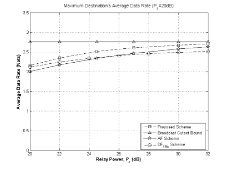

As expected, the proposed strategy (the optimal scheme) outperforms the and schemes. Note that, the superiority of the proposed scheme over is obvious since is a special case of the proposed scheme. The important observation in these figures is that the infinite multilevel strategy is strictly superior to the strategy, which was previously the best known scheme for this setup at the high SNR [25]. However, as the SNR at the relay side increases, the performance of approaches the optimal performance. Furthermore, as increases, the proposed scheme approaches the cutset bound which means that for high values of the relay does not need to be “complicated”. Another observation from these figures is that, as decreases, approaches the optimal performance. This can be explained as follows: when the power of the relay is much smaller than the source power, the relay-destination link limits the performance. Therefore, even using a one-level code at the source is sufficient to deliver an average rate of to the relay, which is the maximum rate that relay can transmit to the destination333Note that even if relay receives a rate more than , the extra rate should be discarded..
VI Conclusion
In this paper, a two-hop network in which the data is transmitted from the source node via a single relay to a destination node was considered. It was assumed that the knowledge of the channel for each hop is not available at the corresponding transmitter. The relay was assumed to be simple, i.e., not capable of data buffering over multiple coding blocks, water-filling over time, or rescheduling. For this network setup, we proposed an infinite-level coding scheme at the source and the relay. It is shown that this scheme in conjunction with the Decode and Forward () relaying is indeed the optimal strategy for maximizing the average data rate received at the destination. We also proposed an algorithm to find the optimum amount of power which should be assigned to each code level at the source and relay. The optimality of the multilevel coding strategy is also verified through numerical results by showing its superiority over the Amplify and Forward () scheme, which was previously the best known scheme for the high SNR regime.
References
- [1] E.C. van der Meulen, “Three-terminal communication channels,” Adv. Appl. Prob, vol. 3, no. 1, pp. 120–154, 1971.
- [2] T. Cover and A. A. El Gamal, “Capacity Theorems for the Relay Channel,” IEEE Trans. Inform. Theory, vol. 25, pp. 572– 584, Sep. 1979.
- [3] B. Schein and R. G. Gallager, “The Gaussian parallel relay network,” in IEEE Int. Symp. Inform. Theory (ISIT), 2000, p. 22.
- [4] M. Gastpar and M. Vetterli, “On the capacity of large Gaussian relay networks,” IEEE Trans. Inform. Theory, vol. 51, no. 3, pp. 765–779, 2005.
- [5] S. Zahedi, M. Mohseni, and A. El Gamal, “On the Capacity of AWGN Relay Channels with Linear Relaying Functions,” in IEEE Intern. Symp. Inform. Theory (ISIT), 2004, p. 399.
- [6] A. ElGamal, M. Mohseni, and S. Zahedi, “Bounds on Capacity and Minimum Energy-Per-Bit for AWGN Relay Channels,” IEEE Trans. Inform. Theory, vol. 52, no. 4, pp. 1545–1561, 2006.
- [7] H. Bolcskei, R.U. Nabar, O. Oyman, and A.J. Paulraj, “Capacity Scaling Laws in MIMO Relay Networks,” IEEE Trans. Wireless Communications, vol. 5, no. 6, pp. 1433–1444, 2006.
- [8] S.O. Gharan, A. Bayesteh, and A.K. Khandani, “Asymptotic Analysis of Amplify and Forward Relaying in a Parallel MIMO Relay Network,” Submitted to IEEE Trans. Inform. Theory, 2008, also available online at http://cst.uwaterloo.ca/pub_jour.html.
- [9] J. N. Laneman, D. N. C. Tse, and G. W. Wornell, “Cooperative diversity in wireless networks: efficient protocols and outage behavior,” IEEE Trans. Inform. Theory, vol. 50, no. 12, pp. 3062–3080, Dec. 2004.
- [10] K. Azarian, H. El Gamal, and Ph. Schniter, “On the Achievable Diversity-Multiplexing Tradeoff in Half-Duplex Cooperative Channels,” IEEE Trans. Inform. Theory, vol. 51, no. 12, pp. 4152–4172, Dec. 2005.
- [11] S. Yang and J.-C. Belfiore, “Towards the optimal amplify-and-forward cooperative diversity scheme,” IEEE Trans. Inform. Theory, vol. 53, pp. 3114–3126, Sept. 2007.
- [12] K. Sreeram, S. Birenjith and P. Vijay Kumar, “Multi-hop cooperative wireless networks: diversity multiplexing tradeoff and optimal code design,” Available online at http://arxiv.org/pdf/0802.1888, February 2008.
- [13] S.O. Gharan, A. Bayesteh, and A. K. Khandani, “Diversity-Multiplexing Tradeoff in the Multiple Relay Network,” Submitted to IEEE Trans. Inform. Theory, 2008, also available online at http://cst.uwaterloo.ca/pub_jour.html.
- [14] S. Pawar, S. Avestimehr and D. N. C. Tse, “Diversity multiplexing tradeoff of the half-duplex relay channel,” in Proceedings of Allerton Conference on Communication, Control, and computing, 2008.
- [15] E. Biglieri, J. Proakis, and S. Shamai, “Fading channels: information-theoretic and communications aspects,” IEEE Trans. Inform. Theory, vol. 44, no. 6, pp. 2619–2692, 1998.
- [16] S. Shamai, “A Broadcast Strategy for the Gaussian Slowly Fading Channel,” in IEEE Intern. Symp. on Inform. Theory (ISIT), Ulm, Germany, Jul. 1997.
- [17] A. Steiner, and S. Shamai, “Achievable Rates with Imperfect Transmitter Side Information Using a Broadcast Transmission Strategy,” IEEE Trans. Wireless Communications, vol. 7, no. 3, pp. 1043–1051, 2008.
- [18] T.T. Kim and M. Skoglund, “On the Expected Rate of Slowly Fading Channels With Quantized Side Information,” IEEE Trans. Communications, vol. 55, no. 4, pp. 820, 2007.
- [19] S. Ekbatani, F. Etemadi, and H. Jafarkhani, “Transmission Over Slowly Fading Channels Using Unreliable Quantized Feedback,” in IEEE Data Compression Conf., March 2007.
- [20] S.R. Mirghaderi, A. Bayesteh, and A.K. Khandani, “On the Capacity of Wireless Multicast Networks,” Submitted to IEEE Trans. Inform. Theory, Arxiv preprint arXiv:0805.4248, also available online at http://cst.uwaterloo.ca/pub_jour.html.
- [21] A. Steiner and S. Shamai, “Multi-Layer Broadcast Hybrid-ARQ Strategies,” in 2008 IEEE Intern. Zurich Seminar on Communications, 2008, pp. 148–151.
- [22] S. Shamai and A. Steiner, “A Broadcast Approach for a Single-User Slowly Fading MIMO Channel,” IEEE Trans. Inform. Theory, vol. 49, pp. 2617– 2635, Oct. 2003.
- [23] A. Steiner, and S. Shamai , “Multi-Layer Broadcasting over a Block Fading MIMO Channel,” IEEE Trans. Wireless Communications, vol. 6, no. 11, pp. 3937–3945, 2007.
- [24] V. Pourahmadi, S.A. Motahari, and A.K. Khandani, “Infinite-level Codes for Single-User Slowly Fading MIMO Shannels,” Accepted in IEEE Int. Symp. Inform. Theory (ISIT), June 2009.
- [25] A. Steiner and S. Shamai, “Single- User Broadcasting Protocols Over a Two- Hop Relay Fading Channel,” IEEE Trans. Inform. Theory, vol. 52, pp. 4821– 4838, Nov. 2006.
- [26] I. E. Telatar, “Capacity of Multi-Antenna Gaussian Channels,” Tech. Rep., Bell Labs, Lucent Technologies, [Online] Available: http://mars.bell-labs.com/papers/proof/proof.pdf, 1995.
- [27] P. Bergmans, “A Simple Converse for Broadcast Channels with Additive White Gaussian Noise,” IEEE Trans. Inform. Theory, vol. 2, pp. 279– 280, Mar. 1974.
- [28] I. Geldfand and S. Fomin, Calculus of Variations, Printice-Hall Inc., 1963.
- [29] Gilbert Strang, “Calculus of Variations,” MIT OpenCourseware, Spring 2006.