Impact of Scale Dependent Bias and Nonlinear Structure Growth on Integrated Sachs-Wolfe Effect: Angular Power Spectra
Abstract
We investigate the impact of nonlinear evolution of the gravitational potentials in the LCDM model on the Integrated Sachs-Wolfe (ISW) contribution to the CMB temperature power spectrum, and on the cross-power spectrum of the CMB and a set of biased tracers of the mass. We use an ensemble of -body simulations to directly follow the potentials and compare the results to analytic perturbation theory (PT) methods. The predictions from the PT match the results to high precision for . We compute the nonlinear corrections to the angular power spectrum and find them to be of linear theory for . These corrections are swamped by the cosmic variance. On scales the departures are more significant, however the CMB signal is more than a factor larger at this scale. Nonlinear ISW effects therefore play no role in shaping the CMB power spectrum for . We analyze the CMB–density tracer cross-spectrum using simulations and renormalized bias PT, and find good agreement. The usual assumption is that nonlinear evolution enhances the growth of structure and counteracts the linear ISW on small scales, leading to a change in sign of the CMB-LSS cross-spectrum at small scales. However, PT analysis suggests that this trend reverses at late times when the logarithmic growth rate or . Numerical results confirm these expectations and we find no sign change in ISW-LSS cross-power for low redshifts. Corrections due to nonlinearity and scale dependence of the bias are found to be for , therefore below the signal-to-noise of the current and future measurements. Finally, we estimate the cross-correlation coefficient between the CMB and halos and show that it can be made to match that for the dark matter and CMB to within for thin redshift shells, thus mitigating the need to model bias evolution.
I Introduction
Measurements of the temperature fluctuations in the Cosmic Microwave Background (CMB), provide a unique window onto the primordial Universe and a means to learn about the physical processes that generated the initial conditions. This discriminatory power is exemplified by recent results from the WMAP experiment (Komatsu et al., 2008): the primordial power spectral index is , ruling out the Harrison-Zel’Dovich spectrum at 3 level. However, the temperature power spectrum does not provide a pristine window, but it must be cleaned for the imprint of foreground signals. One cosmological foreground, is the change in energy that a CMB photon experiences as it propagates through an inhomogeneous Universe with time evolving gravitational potentials, . There are three main effects that may give rise to such secondary fluctuations:
-
•
Linear Integrated Sachs–Wolfe Effect(Sachs and Wolfe, 1967, hereafter ISW): unless the growth of density perturbations matches the expansion rate, will evolve from zero. This will lead to a net change in photon temperatures. In LCDM as the potential decays, giving rise to a net positive correlation between density and temperature in Fourier space.
-
•
Rees–Sciama Effect(Rees and Sciama, 1968, hereafter RS): nonlinear collapse of perturbations to filaments and clusters leads to even in the absence of linear ISW, and CMB photons change energy as they transit across nonlinear structures. It is usually assumed that nonlinear evolution accelerates the growth of structure and counteracts the linear decay of gravitational potential in LCDM. In this paper we show that this is not always justified.
-
•
Birkinshaw–Gull Effect(Birkinshaw and Gull, 1983, hereafter BG): if a mass concentration moves transversely to the line of sight, it will create a time variation in the potential even if the potential itself is not evolving in time, and this will have a dipolar pattern. Consequently, photons which enter the potential in the wake, will receive a net energy boost on exit, and those which enter ahead will loose energy on exit. However, unlike the previous two effects, this contributes only to the CMB auto-correlation and not to the cross-correlation of CMB with a density tracer.
All three effects combine into the nonlinear ISW. It is well known that the linear ISW effect leads to fluctuations of the order on the largest scales for LCDM (see for example Dodelson, 2003) and has been used to rule out the self-accelerating branch of DGP model (Fang et al., 2008).
The impact of the nonlinear evolution of on the CMB has been the subject of a number of studies. However, most of these works attempt to quantify the effect through the use of simplified analytic models (Rees and Sciama, 1968; Kaiser, 1982; Martinez-Gonzalez et al., 1990; Martínez-González et al., 1992; Martinez-Gonzalez et al., 1994; Cooray, 2002a, b). A number of studies have employed numerical simulations to track the evolution of : in a pioneering study, Tuluie and Laguna (1995) and Tuluie et al. (1996) used ray tracing methods to compute the change in temperature for individual photon bundles propagating through inhomogeneous universes. They found that the combined imprint on the CMB power spectrum, due to the RS and BG effects, were of the order on angular scales . Owing to the limited size of their simulations, they were unable to comment on the effects on the lower multipoles. Seljak (1996) related to density and momentum using the Poisson and continuity equation. These predictions were compared to an -body simulation of the then favored SCDM model, and good agreement was found between the two as well as to those of Tuluie et al. (1996). However, these results were obtained in the context of model, where no linear ISW exists, and they could not address behavior, owing to the limited dynamic range of the simulations. Puchades et al. (2006) also recently addressed this problem, but again attention was focused on the large multipole regime.
In a more recent study, Cai et al. (2008) used a single -body simulation, the L-BASIC simulation, which has and comoving length of , to compute the nonlinear ISW effect. They measured the power spectra at each epoch in the simulation and developed an empirical fitting formula for the deviations from linear theory. Using this model they computed the CMB angular power spectrum and found, on scales , that there was significant nonlinear amplification of power, qualitatively confirming the earlier halo model predictions of Cooray (2002a). However, these nonlinear corrections occur on angular scales where the primary anisotropy spectrum is more than two orders of magnitude larger, rendering them of negligible importance. Cai et al. (2008) also found that there was no evidence for deviations for multipoles . One of the aims of this paper is to place more precise constraints on the expected level of contamination on these large scales.
The temperature fluctuations induced through the evolving can also be observed by correlating the CMB against density perturbations, as pointed out by Crittenden and Turok (1996), and the large-scale ISW effect provides an important test for Dark Energy and the curvature of the Universe. This information can be extracted through the cross-correlation of the CMB with tracers of the Large-Scale Structure (hereafter LSS). This analysis has recently been performed by a number of groups using the WMAP data and several large-scale structure measurements (e.g. SDSS, NVSS, 2MASS). This work has resulted in up to level detections of the ISW effect (Scranton et al., 2003; Boughn and Crittenden, 2004; Afshordi et al., 2004; Padmanabhan et al., 2005; Cabré et al., 2006; Giannantonio et al., 2006; Rassat et al., 2007; Giannantonio et al., 2008; Ho et al., 2008). In the near future these detections will be improved upon with PLANCK and the new wide field LSS surveys, such as BOSS, DES, Pan-STARRS-1 and EUCLID, etc.. However, in a recent paper Granett et al. (2008a) measured the cross-correlation between superstructures and super-voids with the CMB. On stacking the signal they found a detection, in multiple WMAP bands, and the sign of which appeared consistent with late time ISW. This appears in stark contrast to expectations from simple signal-to-noise calculations within the LCDM model (Crittenden and Turok, 1996; Hernández-Monteagudo, 2008; Douspis et al., 2008; Frommert et al., 2008). A follow up ‘consistency’ test was performed by Granett et al. (2008b), the results of which cast some doubt on the the signal as arising from ISW, at least within the LCDM model. Cai et al. (2008) also investigated the ISW-density cross-correlations, focusing on the nonlinearities arising from the mass evolution. They found that there was no evidence for enhancement of evolution of , in agreement with the earlier work of Verde and Spergel (2002). One of the questions we shall address in this paper is whether selecting biased tracers of LSS relative to the mass distribution can influence the detection sensitivity for the ISW.
We pursue a two-pronged attack on all of these problems. Our first avenue will be to use a large ensemble of -body simulations to directly follow the evolution of . Our second line is analytic, and we use the nonlinear gravitational perturbation theory (PT) and renormalized bias frameworks to compute all measured quantities. This will help us to provide physical insight into the results along the way.
The paper breaks down as follows: In §II we summarize the basic theory of the ISW. In §III we describe the ensemble of simulations that we use, and describe our estimator for measuring from the simulations. Here we also present maps, comparing the time evolution of density, and in the simulations. In §IV we investigate the two-point statistics of , and besides the usual linear analysis we derive nonlinear expressions within the context of the gravitational perturbation theory. We evaluate the theory and compare directly with measurements from the simulations. Then in §V we compute the impact on the CMB temperature power spectrum. In §VI we turn to the cross-correlations with dark matter, followed by the correlations with halos in §VII including the effects of scale dependent bias. Again, the theory is compared directly with measurements from the simulations. In §VIII we perform the line-of-sight integrals and compute angular cross-power spectra. Finally, in §IX we summarize our findings and conclude.
II Theoretical background
II.1 The ISW effect
On arrival at the observer, the CMB photons, which are sourced at the surface of last scattering, , are imprinted with two sets of fluctuations: the primary anisotropies, which are induced by the primordial fluctuations, perhaps seeded through the inflationary mechanism; and the secondary anisotropies, which are induced as the photons propagate through the clumpy Universe. The primary anisotropies have been studied in great detail for several decades(and for a review of the important processes see Dodelson, 2003; Weinberg, 2008). There are a number of physical mechanisms that give rise to the generation of secondary anisotropies (for a review see The Planck Collaboration, 2006) and one of these is the redshifting of the photons as they pass through evolving gravitational potentials.
The temperature fluctuation induced by the gravitational redshift may be written as (Sachs and Wolfe, 1967):
| (1) |
where is a unit direction vector on the sphere, is the dimensionless metric perturbation in the Newtonian gauge, which reduces to the usual gravitational potential on small scales, the ‘over dot’ denotes a partial derivative with respect to the coordinate time from the FLRW metric, is the comoving radial geodesic distance , and so may equivalently parameterize time. and denote the time at which the photons are received and emitted (i.e. last scattering), respectively, is the speed of light and is the dimensionless scale factor.
On scales smaller than the horizon, the perturbed Poisson equation enables us to relate potential and matter fluctuations (Peebles, 1980):
| (2) |
where is the mean matter density in the Universe and the density fluctuation is . Poisson’s equation may most easily be solved in Fourier space, upon which we have,
| (3) |
However, what we are really interested in is the instantaneous time rate of change of the potential,
| (4) | |||||
| (5) |
where is a time independent quantity in the matter dominated epoch. In the above, we also defined and , with . All quantities with a subscript are to be evaluated at the present epoch. Estimating the change in the photon temperature due to the evolving potentials requires knowledge of the evolution of the density perturbation and its time rate of change. In the linear regime we may solve the equation of motion for exactly and obtain both of these quantities. However, in the nonlinear regime the situation is more complex and requires numerical simulations or nonlinear models to proceed. In simulations, measuring is relatively straightforward, whereas its time derivative is more complicated. As was shown by Seljak (1996) one may obtain this from the perturbed continuity equation (Peebles, 1980):
| (6) |
where is the proper peculiar velocity field. On defining the pseudo-peculiar momentum field to be,
| (7) |
then in Fourier space we may solve the continuity equation directly to give us:
| (8) |
Hence, our final expression becomes,
| (9) |
where to enable us to pass easily from potential to density we introduced the quantity
| (10) |
III The ISW from -body simulations
III.1 The zHORIZON simulations
In this study we use a subset of the Zürich Horizon, “zHORIZON”, simulations. These are a large ensemble of pure cold dark matter -body simulations (), performed at the University of Zürich on the zBOX2 and zBOX3 super-computers. The specific aim for these simulations is to provide high precision measurements of cosmic structures on scales of the order and to also provide insight into the rarest fluctuations within the LCDM model that we should expect to find within the observable universe. In this paper we shall only employ the first 8 zHORIZON simulations, since these runs have 11 snapshots logarithmically spaced in the expansion factor from to , thus giving sufficient time sampling of the simulated density field to capture the late time evolution. The expansion factors at which snapshots are recorded are: .
Each numerical simulation was performed using the publicly available Gadget-2 code (Springel, 2005), and followed the nonlinear evolution under gravity of equal mass particles in a comoving cube of length . All of the simulations were run within the same cosmological model, and the particular choice for the parameters was inspired by results from the WMAP experiment (Spergel et al., 2003, 2007; Komatsu et al., 2008). The parameters are: , where these are: the density parameters in matter, dark energy and baryons; the power spectrum normalization and primordial spectral index; equation of state parameter for dark energy ; dimensionless Hubble parameter. The transfer function for the simulations was generated using the publicly available cmbfast code (Seljak and Zaldarriaga, 1996; Seljak et al., 2003), with high sampling of the spatial frequencies on large scales. Initial conditions were lain down at redshift using the serial version of the publicly available 2LPT code (Scoccimarro, 1998; Crocce et al., 2006).
Dark matter halo catalogs were generated for all snapshots of each simulation using the Friends-of-Friends (FoF) algorithm (Davis et al., 1985), with the linking-length parameter set to the standard . For this we used the fast parallel B-FoF code, kindly provided by V. Springel. The minimum number of particles for which an object was considered to be a bound halo, was set to 30 particles. This gave a minimum host halo mass of .
III.2 Estimating the ISW effect in simulations
In order to estimate , we require estimates of both the density field and pseudo-peculiar momentum field in Fourier space (c.f. Eq. (9). The dark matter density field can be written as a sum over Dirac delta functions,
| (11) |
where is the mass of the th particle and we take all particles to have equal mass. The density field averaged on a cubical lattice can then be obtained through the convolution,
| (12) | |||||
where represents the dimensionless window function of the mass assignment scheme, and where the normalization factor is . The filter function that we adopt throughout is the ‘cloud-in-cell’ charge assignment scheme (Hockney and Eastwood, 1988). Hence, our estimate for the density fluctuation is
| (13) | |||||
where is the total number of grid cells.
The pseudo-momentum field may be estimated in a similar fashion. For convenience we write,
| (14) |
where is the comoving peculiar velocity field. The particle momentum field is then written as
| (15) |
This may be convolved with the mass assignment scheme to obtain the mesh averaged quantity
| (16) |
Thus our estimate for the pseudo-momentum field is given by
| (17) |
The density Fourier modes were then estimated using the publicly available FFTW routines (Johnson and Frigo, 2008), and each resulting mode was corrected for the convolution with the mass-assignment window function. For the CIC algorithm this corresponds to the following operation:
| (18) |
where
| (19) |
and where sub-script d and g denote discrete and grid quantities, and where is the Nyquist frequency, and is the number of grid cells (Hockney and Eastwood, 1988).
To obtain the real space , we solved for in Fourier space using Eq. (9), set the unobservable mode to zero, and inverse transformed back to real space.
III.3 Visual representation of the evolution of
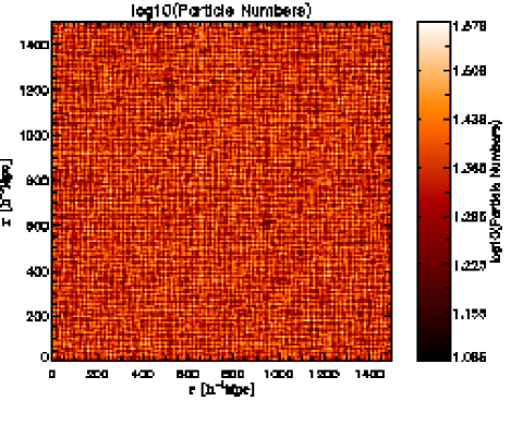
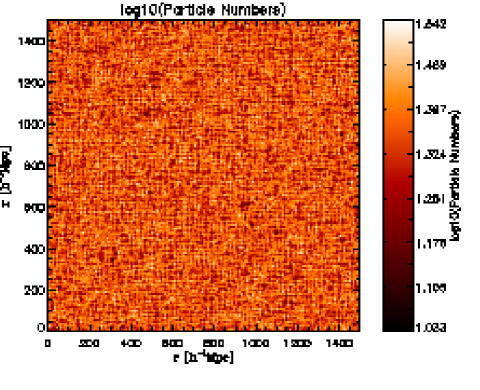
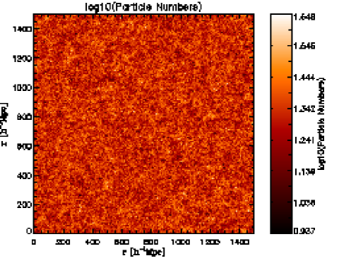
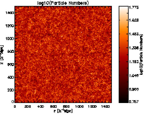
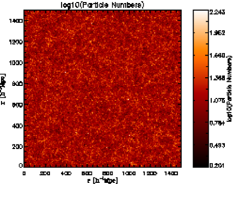
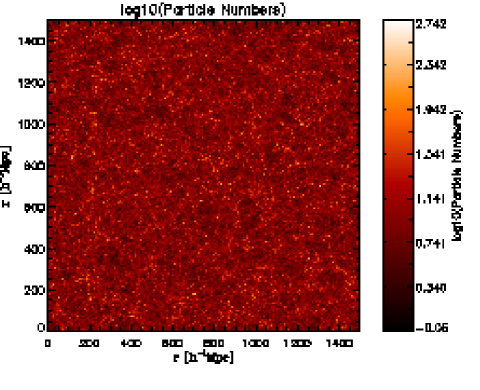
Fig. 1 shows how the dark matter particle number, projected in a slab of thickness and side length , evolves as a function of cosmic time from to the present day. At early times, one can see that the Universe is regular and homogeneous, and the imprint of the initial grid configuration is still noticeable. At later times, gravitational instability of the matter has led to the formation of a pattern of web like structures with dense clumps at the vertices of the web – the ‘Cosmic Web’. The point we wish to stress, is that it is difficult for the eye to pick out features that are larger than .
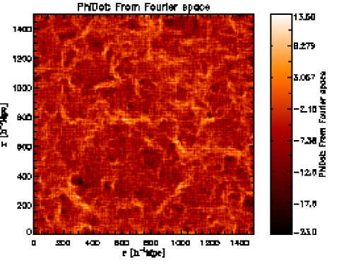
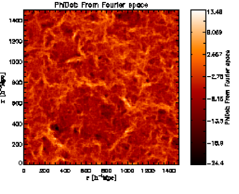
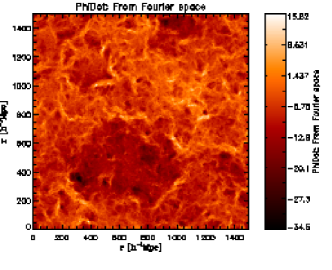
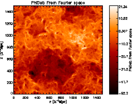
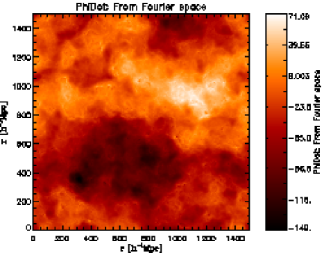
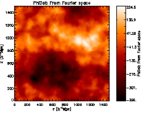
Fig. 2 shows the evolution of as a function of cosmic time. At early times (), when there is no linear ISW, the maps are dominated by a small-scale foam-like structure. At later times, , the foam is sharpened and transformed, with butterfly like features present at the high density regions, as expected from the BG effect, i.e. a flow of mass moving transversely across the sky. At later times the dominating structures are on extremely large scales (), as expected by the linear late time ISW effect.
IV Density, momentum and potential power spectra in PT
IV.1 The 3D power spectra
The perturbed fields of interest may be written as Fourier series,
| (20) | |||||
| (21) |
where , and where is some large region of the Universe over which we shall assume that the functions obey harmonic boundary conditions. Then, from translational invariance and isotropy, the correlation of different Fourier modes can be written
| (22) |
where is the power spectrum matrix of all of the fields. Using Eq. (9) we find, for example:
| (23) | |||||
| (24) |
where we have defined .
IV.2 Linear theory results
The two-point statistics may be evaluated easily within the linear theory: and . In this limit the Fourier mode of the density and its time derivative evolve as:
| (25) | |||||
| (26) |
where we have the usual definition of the logarithmic derivative of the growth factor,
| (27) |
Hence we have
| (28) | |||||
and
| (29) | |||||
Inserting these expressions into Eqs (23) and (24) gives:
| (30) | |||||
| (31) |
At this point we may note the well known result that, if the Universe is in an Einstein–de Sitter (EdS) phase of expansion (i.e. , and ), then and the bracketed terms in Eqs (30) and (31) vanish, so the ISW effect vanishes. However, if the Universe is under/overdense in gravitationally active matter, then we expect a non-zero signal, which is positive for both spectra. In the currently favored LCDM model, , and so . However, at early times and the ISW is shut off. In the next section we explore how this picture changes as the fields are evolved into the mildly nonlinear regime.
Before moving on though, we point out that in the literature there are a number of commonly used approximations for : for example, (Peebles, 1980); and somewhat better, (Lahav et al., 1991) for models with a cosmological constant ; and better still the previous formula, but with the power-index of the first term (Fry, 1985; Hamilton, 2001). However, all these approximations deviate at the few percent level when compared to the exact result obtained from numerically solving the differential equation for linear growth (for further details see for example Hamilton, 2001; Linder and Jenkins, 2003). We therefore adopt the exact numerical solutions for both and throughout this study.
IV.3 Beyond linear theory: Nonlinear PT
The collapse of cosmic structures can be followed into the nonlinear regime using standard perturbation theory (PT) methods, applied to an ideal fluid in a uniformly expanding spacetime (for an excellent review see Bernardeau et al., 2002). The first application of PT methods to estimate the impact of the nonlinear evolution of on the CMB, was given by Seljak (1996). That work was conducted within the context of the flat SCDM model, and hence only provided an estimate for the Rees-Sciama contribution. Furthermore, owing to the fact that at all times in the EdS model, it was necessary only to calculate the PT up to 2nd order in , whereas in more general cosmologies, to be consistent at first order, one requires the corrections up to 3rd order. We shall now calculate the nonlinear ISW in the PT framework for the LCDM model.
To begin, we require from the PT theory the solutions for the fluid overdensity, and in Fourier space these may be written as,
| (32) |
where the perturbative solutions at each order can be written
| (33) |
In the above expression represents an initial field at wavenumber , and the th order perturbed density depends on initial fields. The quantities represent the standard PT interaction kernels, symmetrized in all of their arguments. Also we have adopted the short-hand notation . The Dirac delta function ensures that the waves conserve momenta through the interaction, i.e. . For example, the second order PT kernel can be written,
| (34) |
where .
In the standard approach of nonlinear PT, the fluid equations are solved for the flat EdS background model. In this case the spatial and temporal parts of the evolution are fully separable and the perturbative solutions at each order simply scale as powers of the expansion factor (Jain and Bertschinger, 1994). However, this is not the case for more general cosmological models, nevertheless a very good approximation to the evolution can be obtained by replacing the powers of . Strictly speaking, the PT interaction kernels also inherit some time dependence, however this is an extremely weak function of time and so to a very good approximation we may use the kernels from the flat EdS case (for deeper discussion of this see Bernardeau et al., 2002).
As Seljak (1996) showed, to calculate the ISW we simply require the PT expansion for and its time derivative. Using Eq. (32), this latter quantity may be written,
| (35) |
These quantities may now be used to compute the Next-to-Leading-Order (NLO) corrections to the power spectra. Using the above expressions plus the standard PT techniques we find, for pseudo-momentum:
| (36) | |||||
| (37) |
where the one-loop corrections are,
| (38) | |||||
| (39) |
For the we find:
| (40) | |||||
| (41) |
where the one-loop corrections are,
| (42) | |||||
| (43) |
In the above expression and are the NLO corrections to the matter power spectrum and we defined, (for explicit forms for the 1Loop expressions, see Jain and Bertschinger, 1994; Scoccimarro and Frieman, 1996; Smith et al., 2007).
We may now learn how the NLO corrections entangle the pure linear ISW decay of potentials with the nonlinear RS effects. The easiest way to discern the changes is to consider the sign of the corrections in the above equations. We notice that there are two ways the sign may change: firstly, there is a sign flip with scale, since is negative and dominant on large scales and is positive and dominant on smaller scales; secondly, the time dependent prefactors may change sign.
| Sign of correction | ||
|---|---|---|
Considering the time dependent factors, we see that the cross-power spectrum, Eq.(43), will only change sign when, , which occurs when . We shall label this time . Table 1 summarizes the changes. The key point to notice is that at early times, there is an enhancement of the ISW on very large scales (i.e. enhanced decay of gravitational potentials) and on small scales there is a suppression of ISW effect (growth of potentials). Then, at late times these corrections invert themselves and ISW is suppressed on large scales and small-scale potentials decay.
Turning now attention to the auto-power correction, Eq. (42), we see that the prefactor multiplying is always positive, whereas the second term only switches sign when or . However since , the first bracket will never switch sign and will vanish at early times. On the other hand the second bracket remains negative until . Given current constraints on the second bracketed term is always negative and on multiplying by , we conclude that it too is always positive.
IV.4 Evolution of density power spectrum
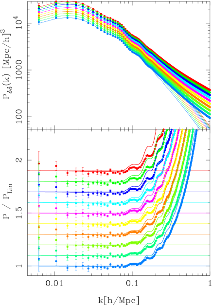
Fig. 3 shows the evolution of the nonlinear matter power spectrum measured from to the present day. The power is plotted from the fundamental mode, to half of the Nyquist frequency of the mesh , where we use for all transforms. Above this frequency the power in the Fourier modes is affected by aliasing from smaller scales (Press et al., 1992). In the top panel we show the mean ensemble averaged absolute power from the simulations at each epoch, colored points with errors. On the largest scales , the power grows by a factor of from to 0, and there appears to be very good agreement with the linear theory predictions on these scales (colored solid lines). On smaller scales the power is significantly amplified.
In the bottom panel of the Fig. 3 we take the ratio of the data with the linear theory, and to see clearly the effects for each snapshot, we offset the curves by 0.1 in the vertical direction, with the solid colored lines being the baseline for each corresponding snapshot. We see that there is a small () suppression of power at late times for modes , this is termed the ‘previrialization feature’ (Smith et al., 2007; Crocce and Scoccimarro, 2008; Angulo et al., 2008). On smaller scales () the power is strongly amplified, compared to linear theory. In this panel we also present the predictions from the standard PT (described in §IV.3) and we see that it qualitatively captures the trends in the data. However, in closer detail, we see that the PT over estimates the power on smaller scales and that the predictions become progressively worse at higher expansion factors and higher wavenumbers.
IV.5 Evolution of the pseudo-momentum spectra
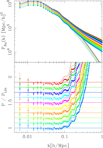
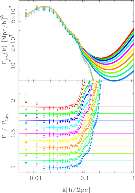
In Figs 4 and 5 we present the pseudo-momentum–density cross- and pseudo-momentum auto-spectra, respectively. Again the top part of each figure shows the absolute power and the bottom the ratio with respect to the linear model (c.f. Eqs 28 and 29). Note that the spectra are amplified relative to the density spectrum, and that on large scales this boost is well captured by multiplicative powers of . In addition, we find that on very large scales, the momentum spectra also display a previrialization feature and that the suppression of power appears to be deeper in both cases. Furthermore, on smaller scales the nonlinear amplification, which occurred at around for , appears at larger scales in both cases, with the , strongly amplified by . We compare these measurements with the predictions from standard PT and find for reasonably good agreement on very large scales and an over prediction on smaller scales. However, for the agreement is much better.
IV.6 Evolution of the power spectra
Having examined the individual components of the spectrum we may now sum them together with weights as given by Eq. (23). Following Seljak (1996) and Cai et al. (2008), we introduce the dimensionless and re-scaled form of ,
| (44) | |||||
| (45) |
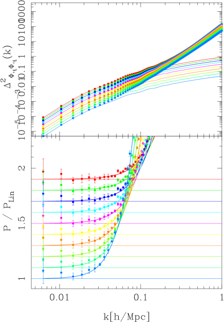
Fig. 6 shows the evolution of the ensemble averaged , with errors on the mean. The top panel shows the absolute spectra for the 10 snapshots from to the present day. Also shown as the thin solid lines are the predictions from the linear theory as given by Eq. (30). Again, there appears to be good agreement on large scales, and nonlinear amplification on smaller scales. The bottom panel presents the ratio with respect to the linear model, again we have offset different epochs by 0.1 in the vertical direction for clarity. There is clear evidence for nonlinear amplification of the spectrum on the very largest scales, and relative to linear theory this becomes increasingly more important at higher redshifts, as expected. Indeed by and at the power is more than 10% in excess of the linear theory prediction, whereas at , a 10% amplification is only achieved by . Here we also show the predictions from the NLO PT calculation from Eqs (40) and (42), and we note a startlingly good agreement at all epochs.
That the nonlinear effects become increasingly important at higher redshifts follows directly from the fact that as . In this case, the only contribution to the spectrum comes from the nonlinear Rees-Sciama effect, and in the limit it is given by
| (46) |
On comparing our results with Fig. 1 from Cai et al. (2008), we find qualitatively good agreement. However, on the largest scales their spectra do not appear to reproduce the linear theory at high precision. The excess signal that they find compared to the linear theory, we believe, is a result of using the approximation . Some of the discrepancy may also be due to cosmic variance, since they only show results for a single simulation. In that work the authors also proposed a nonlinear correction formula for , which has two free parameters. Since the PT has no free parameters, and as it provides an excellent match to the data for the scales we consider our approach a sufficient description on these large scales. Such fitting would most likely be necessary on smaller scales for good agreement, but these scales are of diminishing importance for the calculation of the CMB spectrum for .
V Results: Impact on CMB spectrum
The CMB temperature fluctuations arising from the ISW may be decomposed using a spherical harmonic expansion, and the amplitude of each harmonic can be written as (Cooray, 2002a; Hernández-Monteagudo, 2008),
| (47) |
with,
| (48) |
where we transformed Eq. (1) to comoving geodesic distance and is the distance from the observer to the surface at which the ISW first becomes significant. The power in the harmonic multipoles may be calculated using the standard methods, and the ISW temperature spectrum may be written:
| (49) | |||||
In the limit we may use the Limber approximation to simplify the above integrals (see for example Seljak, 1996; Bartelmann and Schneider, 2001; Cooray, 2002b). Assuming that only modes transverse to the line of sight contribute to the signal and also that the power spectra are slowly varying functions of , then the orthogonality of the spherical Bessel functions gives,
| (50) |
where is the comoving angular diameter distance ( for flat space). On applying this approximation the above expression reduces to the simple form:
| (51) | |||||
| (52) |

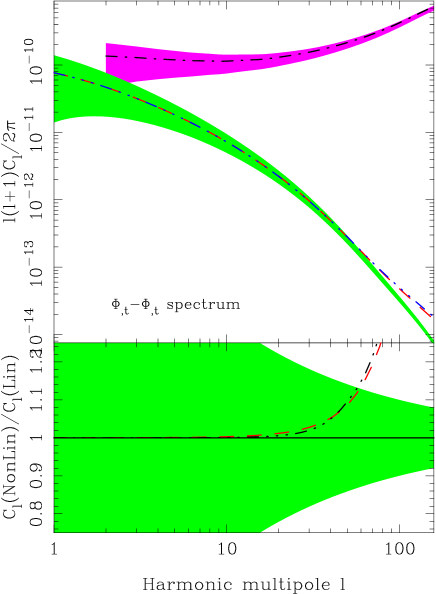
Fig. 7 compares the Limber approximate expressions for the angular power spectrum of temperature fluctuations with the exact spherical harmonic line-of-sight integration. On scales , the Limber approximation is clearly poor with relative errors being . The transformation , as suggested by Ho et al. (2008); Loverde and Afshordi (2008), improves the approximation, but the errors still remain large. However for , the error is reduced and by it is of the order (for a detailed discussion on the validity of the Limber approximation for different power spectra, see Appendix A). We shall nevertheless adopt the Limber approximation for our theoretical analysis, but note that if significant effects are apparent on multipoles , then only a full spherical harmonic analysis will give robust results. However, this would necessarily involve computing the unequal time correlations of the Fourier modes of .
Fig. 8 shows the results for the Limber approximated ISW temperature angular auto-power spectrum. We scale the spectrum by in the usual way and restrict our attention to angular modes . In the upper panel of the figure we compare three predictions: the linear theory calculation with 1- cosmic variance errors, denoted by the green shaded region; the nonlinear PT, denoted by the red dash line; and the mean measurement from the -body simulations blue triple dot-dash curve. The 1- green shaded error region was computed using the Gaussian variance formula:
| (53) |
where is the fraction of sky covered, and we shall take this to be of order unity. The estimate of the spectrum from the -body simulations was obtained by the following prescription: we first made an array of the measured spectra and divided this through by the linear theory ISW power spectrum at that epoch. On very large scales the ratios all asymptotically approach unity and so the only evolution that remains to be modeled is the higher domain. To do this, we employ the bi-cubic spline routine (Press et al., 1992) and interpolate the spectra in and . Note that on scales greater than the fundamental mode of the simulation cube the bi-cubic spline gives unity and we recover exactly linear theory. We emphasize the importance of this step, since otherwise the spectra will be significantly reduced for , owing to the finite volume of the simulations. Note that in order to avoid extrapolating the bicubic spline fits into regions where we have no measured data, the upper redshift limit of the Limber integrals was set to . We have tested that this does not change our results in any significant way, by computing the PT out to .
In Fig. 8, we see that all three theoretical predictions converge for , however for we find enhancement of the signal for both the PT and -body results and that these agree to high precision, in agreement with expectations from Fig. 6. By they both show between increase in the power. We also show the CMB primary anisotropy power spectrum as the black dot-dash line, with the magenta shaded band giving the cosmic variance errors, Eq. (53). The primary spectrum was obtained using the cmbfast routine with cosmological parameters to match those of the zHORIZON simulations. Note that, by default, this spectrum already includes the linear ISW effect.
Comparing the primary with the ISW signal, we see that at the primary signal is two orders of magnitude larger, and so the nonlinear enhancement at these multipoles will induce changes to the CMB spectrum that are . While the nonlinear effect exceeds cosmic variance in ISW for , it never exceeds the cosmic variance from the total CMB, since ISW contribution to CMB decreases with . Our findings are consistent with earlier results (Cooray, 2002b; Cai et al., 2008), but are established with improved precision. We therefore do not expect large-scale nonlinear evolution of the gravitational potentials to be responsible for any anomalies in WMAP angular power spectrum.
VI ISW-dark matter cross-correlation spectrum
Having discussed the ISW auto-correlation spectrum we now move on to discussing ISW correlation with the density field. We begin with the dark matter density . This can be observed by cross-correlating the CMB with the weak lensing signal of galaxies (Seljak and Zaldarriaga, 1999b, a), the weak lensing of 21cm transitions (Zahn and Zaldarriaga, 2006) or the weak lensing of CMB itself (with information encoded in CMB bispectrum) (Goldberg and Spergel, 1999; Verde and Spergel, 2002). In addition, there are a number of advantages to be gained from studying this: firstly, there exists an “alternative” method for estimating , and this provides us with an independent check on our “standard method”, described in §II; secondly, owing to the larger number of dark matter particles, the effects of shot noise on the spectra can be better assessed, and as we will show for the alternate method, more easily corrected for.
VI.1 Alternative estimator for
Our alternative approach to estimating can be understood as follows: Consider the ensemble average of the product of and , using Poisson’s equation we may rewrite this as,
| (54) | |||||
We now take advantage of the useful property that
| (55) |
Through further use of Poisson’s equation, the last term in the above equation may be rewritten in terms of the density power spectrum, i.e. . Putting this together, we arrive at the result (Verde and Spergel, 2002),
| (56) | |||||
where . This simple expression informs us that the ISW cross-correlation can also be estimated from just two things: the matter power spectrum and its evolution with time. We may check that the above expression is consistent with our previous result (c.f. Eq. 24). On assuming linear theory , then we find
| (57) |
and on insertion of the above expression into Eq. (56), we recover our earlier result.
The practical implementation of the above algorithm requires us to estimate the time derivative of the power spectrum, and we do this using the usual time-centered difference scheme:
| (58) |
where is the estimate at epoch . Note that since we employ a time-centered difference scheme, we do not show results for for or , the first and last epochs considered.
VI.2 Results: evolution of
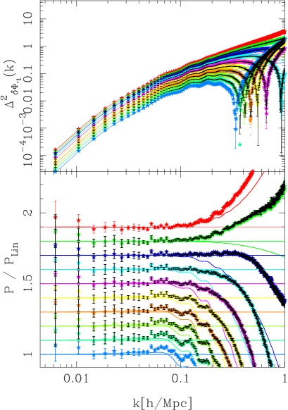
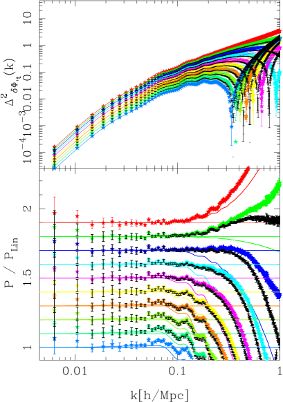
Fig. 9 compares the results for obtained from our standard method (c.f. Eq.24) of solving the continuity equation (black points with errors), with our alternative method (colored points with errors). As was done for we have introduced a dimensionless and scaled form of the cross-power spectrum (c.f. Eq. 45):
| (59) | |||||
| (60) |
The left panel of Fig. 9 shows that the two independent approaches produce results that agree to high precision. We are therefore confident that both methods are consistent and implemented correctly.
The top panel compares the spectra estimated from the simulations (points with error bars) and the linear theory predictions (solid lines). The lower panels show the ratio with respect to the linear predictions. There are a number of important features that we draw attention to: firstly, rather than nonlinear effects becoming increasingly prominent with time, we see that they are stronger at earlier times and on larger scales. The explanation follows our earlier discussion of Fig. 6, and owes to the fact that the linear ISW effect switches off as and , leaving only the RS contributions (c.f. §IV.3).
Next, we note that there is a sign change in the spectra as one goes from low to high . Since we plot the absolute value of the power the sign change is understood to be the point where the signal drops to zero and bounces back up. The scale at which this sign change occurs is a function of time, and it appears on larger scales at higher redshifts (see also Cai et al., 2008). The sign change is due to the fact that the signal becomes dominated by the RS and BG effects. However, for the spectra with we see no sign change over the -range that we consider. Moreover, unlike the lower redshift epochs we see an amplification relative to the linear theory. This means that, at late times in LCDM model, nonlinear evolution can actually enhance the decay of gravitational potentials, consistent with our earlier discussion of the PT (c.f. §IV.3). Further support for the PT interpretation of this phenomenon comes from the fact that if one considers the results at high redshift, then around there is a small amplification of power with respect to the linear model.
In the discussion so far we have neglected the issue of the discreteness correction due to finite number of dark matter particles. It is unclear how to apply the shot noise correction to the momentum density. However, since we know the shot noise correction on the dark matter power spectrum is , where is the number density of dark matter particles, the discreteness effects may be accounted for more easily when using Eq. (56). Fig. 9, right panel, shows the results obtained from this procedure. Whilst we see that the correction reduces the spectra by a small amount for all , we nevertheless see that both the small-scale late-time amplification and early-time large-scale amplification of the remain significant. We are therefore led to conclude that, nonlinear evolution may lead to a small enhancement of the ISW in the LCDM model.
Comparing our results with the measurements of from Cai et al. (2008), we observe that these authors find no such late time amplification. Owing to the fact that we have provided two independent methods to obtain the estimates, and since we have a significantly larger total simulation volume ( times larger) furnishing smaller errors, we believe that our result is robust. In the next section we shall investigate whether selecting highly biased regions may influence these results further.
VII ISW-halo cross-correlation spectrum
The cross-correlation between and a density tracer field is more easily observable than with the density field itself, which so far is limited because of the small area or large errors in the weak lensing reconstruction. One consequence of this is the added complication of needing to understand the bias relation – the mapping from the tracer population to the underlying dark matter density. In this Section we shall explore whether the cross-correlation of with cluster- and group-scale dark matter haloes, measured in the zHORIZON simulations, between , changes the ISW signal in any significant way, beyond a linear bias. From the assumption that all galaxies reside in dark matter haloes, it follows that the large scale clustering properties of any galaxy sample are a weighted average of the halo clustering statistics. Consequently, studying the halo-ISW cross-correlations should provide representative results for a number of plausible surveys. In particular, while we are limited by the mass resolution of our simulations so that our analysis only applies to biased halos with bias , we note that most of the data sets used for ISW detection so far are based on strongly biased tracers Ho et al. (2008); Giannantonio et al. (2008), so our results are applicable to these.
VII.1 Linear Theory
In nearly all ISW studies to date the bias has been assumed to be not only constant in space, but also in time. As discussed in Ho et al. (2008) and more recently Schaefer et al. (2009), if one wishes to go beyond detection and constrain cosmological models with the ISW, then it is likely that this over simplification will introduce a bias in the recovered parameters, especially when redshift selection functions are broad. The next simplest scenario is a time-dependent linear relationship:
| (61) |
where denotes the tracer type, e.g. galaxies, haloes, clusters etc., is a linear bias parameter that varies in time but is independent of scale. In this case the ISW cross-spectra and biased tracer auto-spectra may be easily computed as (cf. Eq. 31):
| (62) | |||||
| (63) |
VII.2 Nonlinear theory for the bias
Several recent theoretical and numerical studies of the bias of dark matter haloes (Cole et al., 2006; Smith et al., 2007; Angulo et al., 2008), have revealed that the linear model is only likely correct on asymptotically large scales. These predictions have been confirmed by several observational studies of the relative bias of different galaxy populations (Percival et al., 2007; Sánchez and Cole, 2008; Cresswell and Percival, 2008). In Smith et al. (2007) it was shown that the scale dependence of halo bias was a strong function of scale for . In that work a physically motivated analytic framework was developed to model these scale changes. A similar approach was independently developed by McDonald (2006a, b). The model utilizes a nonlinear local bias model (Fry and Gaztanaga, 1993; Coles, 1993):
| (64) |
where the constant term from the Taylor expansion was rewritten as . The density field may be expanded using the PT series expansions from §IV.3. As was shown by Smith et al. (2007), if one transforms to Fourier space and collects terms to a fixed order, then the density field of the biased tracers may be written as a fluctuation series of the form:
| (65) | |||||
| (66) | |||||
where is the th order perturbation to the biased tracer density field. The functions are the bias tracer PT kernels, symmetrized in all of their arguments. The kernels are described in Smith et al. (2007). Thus equations (65) and (66) can be used to describe the mildly non-linear evolution of the biased fields to arbitrary order in the dark matter perturbation. There is a subtlety that we have skipped over: in order to facilitate the Taylor expansion of the biased field it was necessary to filter on a scale , and hence all of the kernels depend on the filter scale. To remove the filter dependence we adopt the renormalization scheme suggested by McDonald (2006a, b). The down side of this, is that the parameters may not be derived ab initio, but must be obtained through fitting to measured data and we shall do this in the following section.
Using these relations, along with McDonald’s renormalizations, we find that the ISW–biased density tracer cross- and auto-power spectra may be written:
| (67) | |||||
| (68) |
where the loop corrections are given by,
| (69) | |||||
| (70) | |||||
| (71) |
and where we have introduced the auxiliary functions:
| (72) | |||||
| (73) |
In the above equations we introduced the renormalized bias parameters and the renormalized constant power term . This may be thought of as an arbitrary white noise contribution.
Before moving on, we notice that the sign reversal property of the nonlinear cross-power spectrum of with mass density, remains unchanged. This owes to the fact that changes the scale at which the loop corrections transit from large-scale power suppression to small-scale enhancement (provided loop corrections are small compared to linear theory).
| Mass Range | |||
|---|---|---|---|
| Bin 1 | |||
| Bin 2 |
VII.3 Renormalized halo bias parameters
In order to use the nonlinear bias model we require the time evolution of the bias parameters, and . These can be estimated directly from the simulations in the following way. Firstly, we divided the haloes at each expansion factor into two classes: (Bin 1) group scale dark matter haloes and (Bin 2) cluster scale dark matter haloes (see Table 2 for details).
These mass bins can be faithfully traced within our simulations out to . We choose fixed mass bins at all epochs for simplicity, but a reasonable association can be made between these halo bins and tracer populations such as Luminous Red Galaxies (LRGs) or clusters. Then for each realization we compute the power spectra: , , , and , for all of the snapshots from . The renormalized halo bias parameters were then directly estimated from the data in the following fashion. Firstly, we fit for on the largest scales using an inverse variance estimator of the form:
| (74) | |||||
| (75) |
where and with . Note that we assume that there is little covariances between bins on these large scales. Having obtained , we next obtain our estimate for . Our estimator has exactly the same form as the above equations except for the fact that and and that . The important quantity to specify is,
| (76) |
It will also be useful later on for us to predict , and to do this we are required to additionally estimate the renormalized shot noise term: . This may be obtained directly from our estimates of along with Eq. (68) and by using Eq. (74), but with and and with . Our estimate per mode is
| (77) | |||||
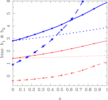
Fig. 10 shows the time evolution of the best fit renormalized halo bias parameters. As is evident from the figure, the values of for the two samples decrease with increasing time. This is qualitatively consistent with the halo bias evolution that emerges from Extended Press-Schechter formalism and the Peak-background split argument (dotted lines), where linear halo bias decays with time as (Fry, 1996; Tegmark and Peebles, 1998; Sheth and Tormen, 1999):
| (78) |
However as the figure clearly shows the actual measured halo bias evolves much more strongly as a function of redshift. We also note that the values of are also similarly consistent with this theory, which predicts that for haloes around (the characteristic nonlinear halo mass at that epoch ), and that for haloes with (Scoccimarro et al., 2001).
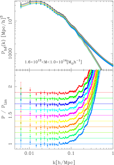
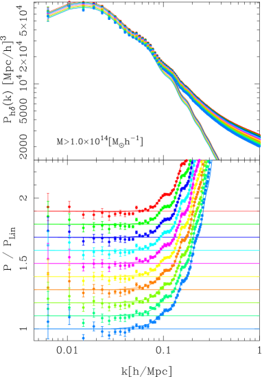
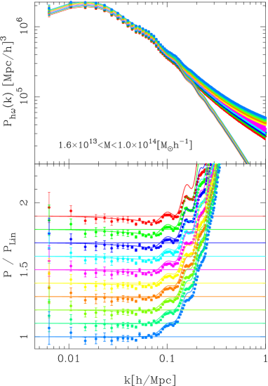
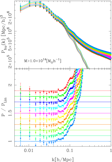
VII.4 Results: Evolution of halo–density spectra
Fig. 12 shows the evolution of in the simulations. The left panel presents the results for haloes in Bin 1 and the right Bin 2. The top sections show the absolute power and the lower sections show the ratio with respect to the linear theory predictions. We observe that all spectra exhibit a strong scale dependence relative to the linear theory and that the departure is characterized by a suppression of power on large scales () followed by power amplification on smaller scales (), and this is exhibited in both mass bins and at all times. The highest mass bin exhibits the strongest amplification with scale, by the spectra are 10% in excess of the linear theory, whereas Bin 1 shows a slightly stronger large-scale power suppression. In the lower sections of each panel in Fig. 12 we also show the predictions of the nonlinear renormalized bias model from § VII.2 and we find surprisingly good agreement over all of the scales of interest. We note that for Bin 1 on the smallest scales , the predictions appear to drop dramatically to zero. However, for the computation of the we expect that this theoretical accuracy will be sufficient. This owes to the fact that the spectra shown in Fig. 12 will all be premultiplied by and so will be suppressed relative to larger scales. We note that the scale dependence of the halo cross-power spectra were investigated by Smith et al. (2007) and we confirm the basic results presented in that study.
VII.5 Results: Evolution of halo–momentum spectra
Fig. 12 shows the evolution of the halo–pseudo-momentum cross-power spectra as a function of scale. Again left and right panels are for Bins 1 and 2, respectively. As expected from our investigation of , we again see nonlinear features in these spectra, and that they are more enhanced relative to those in the spectra. This can be inferred through considering the ratios of the spectra with respect to linear theory (bottom section of each panel). In particular, we note that for Bin 1 and the snapshot, the large-scale suppression feature is of the order at , in contrast to supression in . Again, in the lower panels we over plot the predictions from the renormalized bias model and the agreement is again good, although for small deviations of the model from the data are more apparent. Also, the predictions for Bin 1 drop to zero at higher , and this occurs for the reasons previously noted.
VII.6 Results: Evolution of halo– spectra
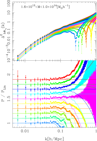
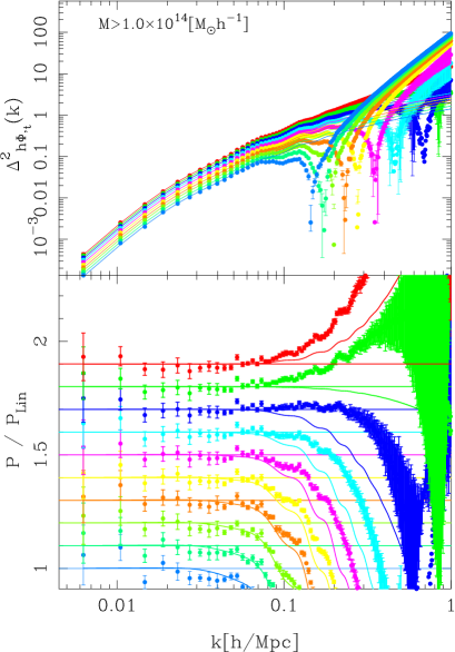
In Fig. 13 we combine the power spectra from the previous two subsections to explore the evolution of . As was done for the analysis of and we introduce a dimensionless and scaled form of the biased cross-power spectrum (c.f. Eq. 45):
| (79) |
The top panels compare the spectra estimated from the simulations (points with error bars) and the linear theory predictions (solid lines). The lower panels show the ratio with respect to the linear predictions, and the lines show the predictions from the renormalized nonlinear bias model. As was the case for our investigation of (c.f. VI.2), departures from linear theory are increasingly apparent as one considers higher redshifts. In addition, there is a sign change in the spectra as one goes from low to high . The explanation again follows our earlier discussions surrounding Figs 6 and 9. On comparing these results for the haloes with those for the dark matter, Fig. 9, we find that the scale at which the spectra switch sign becomes larger with increasing bias.
Considering the small-scale, late-time ISW boost relative to linear theory, we see that for the haloes at the signal is stronger as bias increases. However, we also note that the amplification is present for the Bin 1 halo sample by , compared to the Bin 2 sample where it is absent by . This result means that, at late times in LCDM model, nonlinear evolution can enhance the decay of gravitational potentials and that the rate of decay also depends on the environment. Again, this result naturally emerges from the PT (c.f. §IV.3), although as is shown in the figure, the PT struggles to capture the measured spectra precisely. In the next section we shall investigate whether these nonlinear effects are sufficiently large to impact the ISW-density tracer ’s.
VIII CMB-LSS angular power spectrum
VIII.1 Theory
We now turn to the calculation of the ISW–biased density tracer angular power spectrum. As described in §V for the ISW auto-spectrum, we may also decompose the projected fluctuations in our biased density tracer into spherical harmonics. To do this, we define the 2D biased density field as the weighted projection of the 3D density field along the line of sight and in a cone of solid angle . This we may write as,
| (80) |
where is a radial weight function, which is normalized such that
| (81) |
To proceed we must specify . For a typical magnitude limited survey the weight function would be where is the space density of galaxies above the flux limit at a given redshift, and is the total number of galaxies, and so the number redshift distribution. Therefore, in turn, one is required to specify a model for the redshift distribution (see for example Afshordi et al., 2004; Padmanabhan et al., 2005).
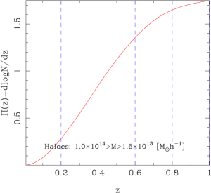
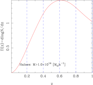
Since we are more interested in precisely quantifying the importance of nonlinear contributions to the cross-correlation signal for biased tracers, which we can measure directly at all epochs in the simulations, we shall therefore forgo attempting to fabricate certain aspects of a real galaxy survey – this level of detail may confuse interpretation. Instead we shall take a more simplified approach: we assume that, above some fixed mass threshold, there is one and only one galaxy (perhaps an LRG) per dark matter halo; that the mass threshold is independent of redshift; and that we may construct a volume limited sample of these objects from out to . This last condition implies that there is a tight relation between the mass threshold of the host halo and the luminosity threshold for the carefully selected target galaxy. Our model galaxy survey is therefore equivalent to a target sample of haloes above some fixed mass from redshift to . Hence, we shall write the weight function, , where is the cumulative number density of dark matter haloes with masses greater than at time ; and where by our normalization condition, for a redshift shell between and we have
| (82) |
In the above, , is the differential halo mass function at time and . Figure 14 shows the redshift distributions of our mock target samples, in the two mass bins and as a function of redshift. In the figure we have introduced the new weight function
| (83) |
where , is the top-hat function with being the Heaviside step function.
The multipole amplitudes of the biased density tracers may therefore be written,
| (84) |
with,
| (85) |
Following Eq. (49), the cross-angular-power of the ISW temperature fluctuations and the projected density tracers may then be written:
| (86) | |||||
Under the Limber approximation (c.f. §V) this expression reduces to:
| (87) | |||||
and for the halo auto-power spectrum we have
| (88) | |||||
In Appendix A we present a short investigation of the validity of the Limber approximation for predicting the ISW-LSS cross-power spectrum. There we show that the relative error is for and that for it is , and for a wide range of survey window functions. These results are consistent with the findings of Rassat et al. (2007) for the 2MASS survey. Since we are interested in scales , we shall therefore use the Limber approximated expressions.
VIII.2 Results: ISW–biased tracer angular spectrum
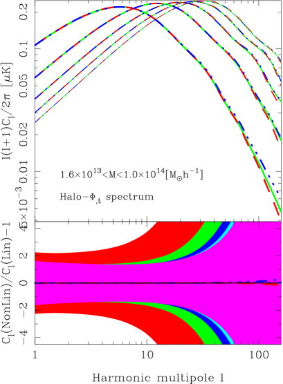
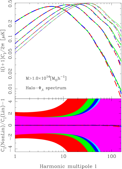
Figure 15 presents the results for the angular cross power spectrum for the ISW and haloes in Bin 1 (left panel) and haloes in Bin 2 (right panel). In each case we show the results for 5 narrow bins in redshift, and where for each bin we weight by the redshift distributions presented in Fig. 14. The solid green lines in the figure denote the linear bias predictions; the red dashed lines correspond to our predictions from the nonlinear renormalized PT, as described in §VII.2 and §VII.3; and the blue triple-dot dash lines correspond to our bi-cubic spline fit to the ensemble average measurements of from the simulations, and scaled by linear theory.
In the figure we see that for both Bins 1 and 2 the peak of the angular power spectrum moves to the right and upwards as the mean redshift of the sample increases. The rightward shift is due to the fact that for a given physical scale the angular size decreases with distance, in this case the scale is the peak of the spectrum. The upward shift is more complex, if we were considering unbiased tracers then we would expect that the signal would drop with increasing redshift, owing to the fact that the ISW signal switches off and also the amplitude of the power spectrum is decreasing with . However, for a fixed mass range, the bias of the sample increases with increasing redshift (c.f. Fig. 10). For the two host halo mass bins that we consider the bias evolves by a factor of from –1.
Regarding the impact of nonlinearity on the predictions, we find that for these are small, being at most . For Bin 1, the deviations are characterized by a several percent boost around , followed by a several percent suppression by . Whereas for Bin 2, the deviations are represented as a few percent suppression. For the deviations are, in all but one case, characterized by a much more significant suppression, and the signal rapidly drops to zero. The case which does not conform to this picture is the lowest redshift slice for Bin 1, here the signal estimated from the simulations appears to be boosted by at . Unfortunately, this amplification is not mirrored in the predictions from the PT, as also seen in Fig (13) for the last four spectra.
In Fig. 15 we also show the expected 1– error domains (shaded regions) of the cross-spectra, computed from using the simple variance formula:
| (89) |
As in the case for , we again find that the cosmic and sample variance errors dominate over the modeling errors on scales .
VIII.3 Calculation of the for biased tracers
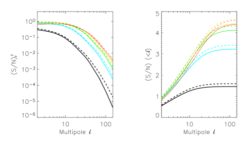
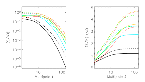
The result from Hernández-Monteagudo (2008) is that for the ISW–dark matter cross-correlation up to of the Signal-to-Noise () for the ISW comes from harmonic modes . Here we shall assess whether sampling biased density tracers can change these conclusions. From the last equation we write the for the ISW–dark matter cross-correlation, at a given multipole , as
| (90) |
Similarly, this equation can be written for the halo distribution,
| (91) |
In the above, no shot noise subtraction on the halo auto-power spectrum is assumed. We can define the cumulative below a given multipole as
| (92) |
This addition is legitimate only under full sky coverage (), since we assume that different multipoles are independent. In the left panel of Fig. 16 we show , for the cluster-mass halo population (Bin 2, solid lines) and the matter density field (dashed lines) for the 5 different redshift shells. The right panel of the figure shows the corresponding cumulative below each multipole . We note that the is flat for low multipoles, and declines rapidly with increasing . The scale at which the turn down occurs is a function of redshift. For the turn down occurs at , whereas for it has dropped by . From studying the cumulative , we find that roughly 50% of the total is achieved by , and that % is achieved by (c.f. Hernández-Monteagudo, 2008). On comparing these results with the corresponding ones for the matter field (dashed lines), we find slightly lower values for the haloes. This may be atributed to the additional Poisson noise. Note that the redshift shell that gives the highest is located at , and that the total for it is of order .
Based on these findings, we conclude that it is highly unlikely that nonlinear evolution of the mass distribution or nonlinearities in the scale dependence of bias can significantly affect the detectability of the ISW.
VIII.4 Results: Cross-correlation coefficient
Finally, we investigate the cross-correlation coefficient of the CMB temperature fluctuations and the halo samples. The cross-correlation coefficient of two fields and is defined as,
| (93) |
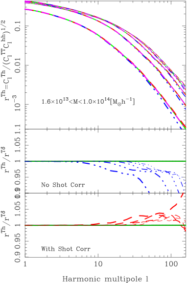
Under the assumption of time independent linear bias we would have . Thus does not depend on the bias of the tracer sample, nor the amplitude of the primordial power spectrum. Instead it provides direct information on the Dark Energy parameters and the curvature density: . This approach was developed by Giannantonio et al. (2008) to obtain cosmological parameter constraints from current CMB and LSS data (see also Zhang, 2006, for an alternate method for removing bias, that uses CMB lensing.).
The validity of this analysis hinges on the fact that cancels out. However, since the bias is in fact time-dependent, we can only have . Adding to this the fact that the bias is scale-dependent it appears that such an approximation is unlikely to be robust, and especially for LSS surveys with broad selection functions. We may test their conjecture by estimating for several samples of biased tracers, and if we do not find that they match within the same redshift shell, then the modeling should be deemed to be insecure. In that case one must include the redshift evolution of the bias, as done by Ho et al. (2008) in their analysis of the NVSS sample.
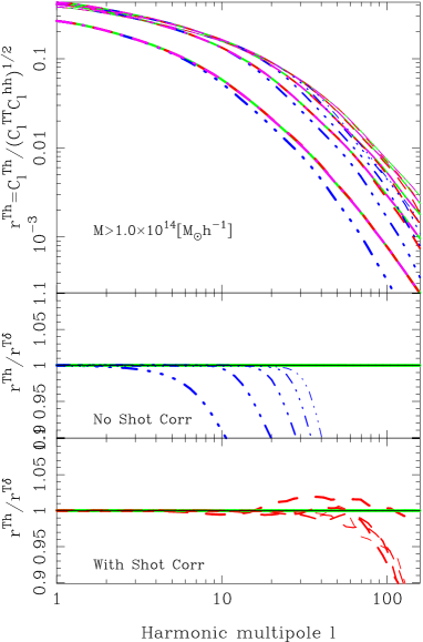
In Fig. 17 we present the measured cross-correlation coefficients for the Bin 1 (left panel) and Bin 2 (right panel) halo samples and for the 5 redshift bins previously considered. The linear theory predictions are represented by the solid green lines and note that for these we use the time-dependent linear bias estimated directly from the simulations. In the figure we also present two different estimates for the full nonlinear cross-correlation coefficient, estimated from bicubic spline fits to the measured spectra: the blue triple-dot dash curves show the results for the case where no shot noise subtraction was performed on the data; the red dash curves show the same but with the shot noise subtracted. We also show the dark matter-CMB cross-correlation coefficient, , measured in the same redshift bins as for the haloes (magenta dot-dash curves). For the dark matter estimates, we used the selection function .
For these narrow redshift shells, , we find that for linear theory, neglecting the evolution of the bias does not lead to significant errors. This can be seen from the middle panels of the figures, where we plot (solid green line for linear theory). However, for the actual measured nonlinear , we find that the scale-dependence of the spectra, leads to a significant discrepancy between and . The discrepancy is at for the lowest redshift cluster-sized halo sample (Bin 2). For the group-scale haloes (Bin 1), the deviation is smaller, being at , for the same redshif shell. However, if one subtracts shot noise from the halo auto-spectra (bottom panel of the figures), , then these effects can be mitigated, and the ratio is brought within of unity. A note of caution, is that we found that using the standard to correct for the shot-noise lead to negative power spectra at high . Since this is forbidden, we believe that such simple corrections are in fact an over-correction and new more accurate methods for accounting for the discreteness will be required (for a deeper discussion of this issue see Smith et al., 2007).
We thus conclude that the relation holds to within for , for the halo samples considerd in this study. This comes under the provision that the shot noise is accounted for and the shells are narrow.
IX Conclusions
In this paper we have investigated the impact of the nonlinear evolution of the time rate of change of the gravitational potentials on the CMB temperature auto-power spectrum, and also on the cross-correlation of biased density tracers and the CMB. Linear perturbation theory informs us that, for nearly the entire history of the Universe, gravitational potentials are constant and there is no net heating or cooling of the primordial CMB photons. However, at late times in the LCDM model the symmetry between the growth rate of density perturbations and the expansion rate is broken. The growth slows, and potentials begin to decay. Using the zHORIZON simulations, a large ensemble of -body simulations and analytic perturbation theory methods, we explored how this picture changed.
In §III we generated maps of the rate of change of the gravitational potentials at different stages in the simulation. We showed that, at redshifts , whilst the ISW signal is vanishingly small, the potentials are indeed evolving nonlinearly on small scales giving rise to the Rees-Sciama and Birkinshaw-Gull effects – nonlinear infall and mass motion across the line of sight. However, the amplitude of these effects, at these redshifts, is too low to be detected directly in the CMB or through a cross-correlation analysis. We then showed that at later times the potential evolution becomes dominated by the large-scale ISW effect.
In §IV we focused on investigating the impact on the CMB temperature power spectrum. The late time ISW effect can be quantified through a line-of-sight integral over three power spectra: the auto-spectra of density and momentum, and their cross-spectrum. We used the nonlinear PT to derive explicit expressions for each of these quantities. Estimates were then measured from the ensemble of simulations over the range –. In all cases there was evidence for large-scale nonlinearity, the effects being strongest for the momentum auto-spectra and at the lowest redshifts. However, when the spectra were combined to produce the spectrum, the nonlinear corrections to linear predictions increased with increasing redshift. This was attributed to the fact that the ISW vanishes at early times, so leaving only the RS and BG effects. The standard PT was able to reproduce the nonlinear behavior at high precision over this redshift range.
In §V we estimated the CMB spectrum using the Limber approximation, we found that the nonlinear amplification of the ISW effect was of the linear theory on scales , and was also swamped by the cosmic variance of the linear ISW effect on these scales. On smaller scales the effect was more significant, however the primary CMB signal is more than times larger at this scale. We conclude that for the standard LCDM model, it is highly unlikely that the nonlinear ISW effects could contaminate the multipoles of the CMB spectrum in any traceable way. Our results support conclusions from earlier studies (Seljak, 1996; Cooray, 2002a; Maturi et al., 2007; Cai et al., 2008).
In §VI we analyzed the cross-correlation of ISW with the dark matter density field, showing that while the nonlinear effects suppress this cross-correlation at early times, they may enhance it at very late times. This is further investigated in §VII, where we computed the ISW signal obtained from the cross-correlation of the CMB with a set of biased tracers of the density field. We modeled the bias using a time dependent linear model and also a time- and scale-dependent nonlinear model (Smith et al., 2007; McDonald, 2006a, b). For the biased samples we took the haloes measured in the simulations between and 1, with masses . These were then sub-divided into a high- and low-mass sample. The linear and nonlinear bias parameters were then estimated from the halo-mass cross-power spectra. The angular power spectrum of the ISW depends on two spectra: the cross-power spectrum of the biased tracer with the mass density and the momentum. These spectra were estimated from the simulations. Again there was evidence for large-scale nonlinearity, the effects being strongest for the momentum cross-spectrum and at late times. The predictions from the nonlinear analytic PT model were found to qualitatively reproduce the power spectra. On combining the two spectra to produce the ISW-density tracer cross-spectrum, we again found evidence of nonlinearity, and as for the case of the ISW auto-spectrum, the effects were more noticeable at higher redshifts. We also found that at late times there was an amplification of the cross-power spectrum. Thus at late times in the LCDM model, nonlinear evolution can lead to a small increase in the decay rate of the gravitational potentials.
In §VIII we computed the angular power spectra, averaging over the halo spectra at various redshifts. We found that on scales the departures from linear theory predictions were , and these were characterized by a small amplification of the signal, followed by a strong suppression. The departures are sub-dominant to the cosmic variance. We then investigated the for the haloes and found good agreement with the linear theory expectation: the presence of bias effectively cancels out in the expression and leads to negligible changes in the cross-correlation detectability. We also showed that through the increased Poisson noise of the biased sample, there was a reduction in the , relative to that for the mass. Our analyses also demonstrated that the of the ISW–large-scale structure cross correlation is localized to a narrow angular range: more than % of the overall significance arises from , or angular scales larger than degrees. We therefore conclude that the current power spectrum analyses of Ho et al. (2008) and Giannantonio et al. (2008) are not affected by nonlinear density evolution or scale-dependent bias to influence the detectability of the ISW-LSS cross-correlation. Since we do not repeat the exact analysis of Granett et al. (2008a) we cannot directly address whether that result can be explained by nonlinear effects or whether it requires an alternative explanation.
Finally, we compared the cross-correlation coefficient of the biased density tracers and the CMB with that of the dark matter and the CMB. We found that the relation holds to within for , for the halo samples considerd in this study. This comes under the provision that the shot noise is accounted for and the shells are narrow. Otherwise the deviations can be large.
The power spectrum anslysis of ISW, therefore, appears to be a probe relatively free from contamination by the pernicious effects of late-time nonlinear evolution of the large-scale structures or scale dependent bias, at least for where most of the signal is. It therefore continues to be a useful probe for the presence of Dark Energy or its alternatives (Lombriser et al., 2009).
Acknowledgments
We acknowledge L. Marian for a careful reading of the draft. RES kindly thanks the Argelander Institute, University of Bonn for hospitality whilst some of this work was being performed. CHM acknowledges the warm hospitality of the University of Zurich, where this work was initiated. We kindly thank V. Springel for making public GADGET-2 and for providing his B-FoF halo finder; R. Scoccimarro for making public his 2LPT code. RES acknowledges support from a Marie Curie Reintegration Grant. This work is partly supported by the Swiss National Foundation under contract 200021-116696/1 and WCU grant R32-2008-000-10130-0.
References
- Komatsu et al. (2008) E. Komatsu, J. Dunkley, M. R. Nolta, C. L. Bennett, B. Gold, G. Hinshaw, N. Jarosik, D. Larson, M. Limon, L. Page, et al., ArXiv e-prints 803 (2008), eprint 0803.0547.
- Sachs and Wolfe (1967) R. K. Sachs and A. M. Wolfe, ApJ 147, 73 (1967).
- Rees and Sciama (1968) M. J. Rees and D. W. Sciama, Nature 217, 511 (1968).
- Birkinshaw and Gull (1983) M. Birkinshaw and S. F. Gull, Nature 302, 315 (1983).
- Dodelson (2003) S. Dodelson, Modern cosmology (Modern cosmology / Scott Dodelson. Amsterdam (Netherlands): Academic Press. ISBN 0-12-219141-2, 2003, XIII + 440 p., 2003).
- Fang et al. (2008) W. Fang, S. Wang, W. Hu, Z. Haiman, L. Hui, and M. May, PRD 78, 103509 (2008), eprint 0808.2208.
- Kaiser (1982) N. Kaiser, MNRAS 198, 1033 (1982).
- Martinez-Gonzalez et al. (1990) E. Martinez-Gonzalez, J. L. Sanz, and J. Silk, ApJL 355, L5 (1990).
- Martínez-González et al. (1992) E. Martínez-González, J. L. Sanz, and J. Silk, PRD 46, 4193 (1992).
- Martinez-Gonzalez et al. (1994) E. Martinez-Gonzalez, J. L. Sanz, and J. Silk, ApJ 436, 1 (1994).
- Cooray (2002a) A. Cooray, PRD 65, 103510 (2002a), eprint arXiv:astro-ph/0112408.
- Cooray (2002b) A. Cooray, PRD 65, 083518 (2002b), eprint arXiv:astro-ph/0109162.
- Tuluie and Laguna (1995) R. Tuluie and P. Laguna, ApJL 445, L73 (1995), eprint arXiv:astro-ph/9501059.
- Tuluie et al. (1996) R. Tuluie, P. Laguna, and P. Anninos, ApJ 463, 15 (1996), eprint arXiv:astro-ph/9510019.
- Seljak (1996) U. Seljak, ApJ 460, 549 (1996), eprint arXiv:astro-ph/9506048.
- Puchades et al. (2006) N. Puchades, M. J. Fullana, J. V. Arnau, and D. Sáez, MNRAS 370, 1849 (2006), eprint arXiv:astro-ph/0605704.
- Cai et al. (2008) Y.-C. Cai, S. Cole, A. Jenkins, and C. Frenk, ArXiv e-prints (2008), eprint 0809.4488.
- Crittenden and Turok (1996) R. G. Crittenden and N. Turok, Physical Review Letters 76, 575 (1996), eprint arXiv:astro-ph/9510072.
- Scranton et al. (2003) R. Scranton, A. J. Connolly, R. C. Nichol, A. Stebbins, I. Szapudi, D. J. Eisenstein, N. Afshordi, T. Budavari, I. Csabai, J. A. Frieman, et al., ArXiv Astrophysics e-prints (2003), eprint arXiv:astro-ph/0307335.
- Boughn and Crittenden (2004) S. Boughn and R. Crittenden, Nature 427, 45 (2004), eprint arXiv:astro-ph/0305001.
- Afshordi et al. (2004) N. Afshordi, Y.-S. Loh, and M. A. Strauss, PRD 69, 083524 (2004), eprint arXiv:astro-ph/0308260.
- Padmanabhan et al. (2005) N. Padmanabhan, C. M. Hirata, U. Seljak, D. J. Schlegel, J. Brinkmann, and D. P. Schneider, PRD 72, 043525 (2005), eprint arXiv:astro-ph/0410360.
- Cabré et al. (2006) A. Cabré, E. Gaztañaga, M. Manera, P. Fosalba, and F. Castander, MNRAS 372, L23 (2006), eprint arXiv:astro-ph/0603690.
- Giannantonio et al. (2006) T. Giannantonio, R. G. Crittenden, R. C. Nichol, R. Scranton, G. T. Richards, A. D. Myers, R. J. Brunner, A. G. Gray, A. J. Connolly, and D. P. Schneider, PRD 74, 063520 (2006), eprint arXiv:astro-ph/0607572.
- Rassat et al. (2007) A. Rassat, K. Land, O. Lahav, and F. B. Abdalla, MNRAS 377, 1085 (2007), eprint arXiv:astro-ph/0610911.
- Giannantonio et al. (2008) T. Giannantonio, R. Scranton, R. G. Crittenden, R. C. Nichol, S. P. Boughn, A. D. Myers, and G. T. Richards, PRD 77, 123520 (2008), eprint 0801.4380.
- Ho et al. (2008) S. Ho, C. Hirata, N. Padmanabhan, U. Seljak, and N. Bahcall, PRD 78, 043519 (2008), eprint 0801.0642.
- Granett et al. (2008a) B. R. Granett, M. C. Neyrinck, and I. Szapudi, ApJL 683, L99 (2008a), eprint 0805.3695.
- Hernández-Monteagudo (2008) C. Hernández-Monteagudo, A&A 490, 15 (2008), eprint 0805.3710.
- Douspis et al. (2008) M. Douspis, P. G. Castro, C. Caprini, and N. Aghanim, A&A 485, 395 (2008), eprint 0802.0983.
- Frommert et al. (2008) M. Frommert, T. A. Enßlin, and F. S. Kitaura, MNRAS 391, 1315 (2008), eprint 0807.0464.
- Granett et al. (2008b) B. R. Granett, M. C. Neyrinck, and I. Szapudi, ArXiv e-prints (2008b), eprint 0812.1025.
- Verde and Spergel (2002) L. Verde and D. N. Spergel, PRD 65, 043007 (2002), eprint arXiv:astro-ph/0108179.
- Weinberg (2008) S. Weinberg, Cosmology (Cosmology, by Steven Weinberg. ISBN 978-0-19-852682-7. Published by Oxford University Press, Oxford, UK, 2008., 2008).
- The Planck Collaboration (2006) The Planck Collaboration, ArXiv Astrophysics e-prints (2006), eprint arXiv:astro-ph/0604069.
- Peebles (1980) P. J. E. Peebles, The large-scale structure of the universe (Research supported by the National Science Foundation. Princeton, N.J., Princeton University Press, 1980. 435 p., 1980).
- Springel (2005) V. Springel, MNRAS 364, 1105 (2005), eprint arXiv:astro-ph/0505010.
- Spergel et al. (2003) D. N. Spergel, L. Verde, H. V. Peiris, E. Komatsu, M. R. Nolta, C. L. Bennett, M. Halpern, G. Hinshaw, N. Jarosik, A. Kogut, et al., ApJS 148, 175 (2003), eprint arXiv:astro-ph/0302209.
- Spergel et al. (2007) D. N. Spergel, R. Bean, O. Doré, M. R. Nolta, C. L. Bennett, J. Dunkley, G. Hinshaw, N. Jarosik, E. Komatsu, L. Page, et al., ApJS 170, 377 (2007), eprint arXiv:astro-ph/0603449.
- Seljak and Zaldarriaga (1996) U. Seljak and M. Zaldarriaga, ApJ 469, 437 (1996), eprint arXiv:astro-ph/9603033.
- Seljak et al. (2003) U. Seljak, N. Sugiyama, M. White, and M. Zaldarriaga, PRD 68, 083507 (2003), eprint arXiv:astro-ph/0306052.
- Scoccimarro (1998) R. Scoccimarro, MNRAS 299, 1097 (1998), eprint arXiv:astro-ph/9711187.
- Crocce et al. (2006) M. Crocce, S. Pueblas, and R. Scoccimarro, MNRAS 373, 369 (2006), eprint arXiv:astro-ph/0606505.
- Davis et al. (1985) M. Davis, G. Efstathiou, C. S. Frenk, and S. D. M. White, ApJ 292, 371 (1985).
- Hockney and Eastwood (1988) R. W. Hockney and J. W. Eastwood, Computer simulation using particles (Bristol: Hilger, 1988, 1988).
- Johnson and Frigo (2008) S. Johnson and M. Frigo, http://www.fftw.org/ (2008).
- Lahav et al. (1991) O. Lahav, P. B. Lilje, J. R. Primack, and M. J. Rees, MNRAS 251, 128 (1991).
- Fry (1985) J. N. Fry, Physics Letters B 158, 211 (1985).
- Hamilton (2001) A. J. S. Hamilton, MNRAS 322, 419 (2001), eprint arXiv:astro-ph/0006089.
- Linder and Jenkins (2003) E. V. Linder and A. Jenkins, MNRAS 346, 573 (2003), eprint arXiv:astro-ph/0305286.
- Bernardeau et al. (2002) F. Bernardeau, S. Colombi, E. Gaztañaga, and R. Scoccimarro, Phys. Rep. 367, 1 (2002), eprint arXiv:astro-ph/0112551.
- Jain and Bertschinger (1994) B. Jain and E. Bertschinger, ApJ 431, 495 (1994), eprint arXiv:astro-ph/9311070.
- Scoccimarro and Frieman (1996) R. Scoccimarro and J. A. Frieman, ApJ 473, 620 (1996), eprint arXiv:astro-ph/9602070.
- Smith et al. (2007) R. E. Smith, R. Scoccimarro, and R. K. Sheth, PRD 75, 063512 (2007), eprint arXiv:astro-ph/0609547.
- Press et al. (1992) W. H. Press, S. A. Teukolsky, W. T. Vetterling, and B. P. Flannery, Numerical recipes in FORTRAN. The art of scientific computing (Cambridge: University Press, —c1992, 2nd ed., 1992).
- Crocce and Scoccimarro (2008) M. Crocce and R. Scoccimarro, PRD 77, 023533 (2008), eprint arXiv:0704.2783.
- Angulo et al. (2008) R. E. Angulo, C. M. Baugh, C. S. Frenk, and C. G. Lacey, MNRAS 383, 755 (2008), eprint arXiv:astro-ph/0702543.
- Bartelmann and Schneider (2001) M. Bartelmann and P. Schneider, Phys. Rep. 340, 291 (2001), eprint arXiv:astro-ph/9912508.
- Loverde and Afshordi (2008) M. Loverde and N. Afshordi, PRD 78, 123506 (2008), eprint 0809.5112.
- Seljak and Zaldarriaga (1999a) U. Seljak and M. Zaldarriaga, PRD 60, 043504 (1999a), eprint arXiv:astro-ph/9811123.
- Seljak and Zaldarriaga (1999b) U. Seljak and M. Zaldarriaga, Physical Review Letters 82, 2636 (1999b), eprint arXiv:astro-ph/9810092.
- Zahn and Zaldarriaga (2006) O. Zahn and M. Zaldarriaga, ApJ 653, 922 (2006), eprint arXiv:astro-ph/0511547.
- Goldberg and Spergel (1999) D. M. Goldberg and D. N. Spergel, PRD 59, 103002 (1999), eprint arXiv:astro-ph/9811251.
- Schaefer et al. (2009) B. M. Schaefer, M. Douspis, and N. Aghanim, ArXiv e-prints (2009), eprint 0903.4288.
- Cole et al. (2006) S. Cole, A. G. Sanchez, and S. Wilkins, ArXiv Astrophysics e-prints (2006), eprint arXiv:astro-ph/0611178.
- Percival et al. (2007) W. J. Percival, R. C. Nichol, D. J. Eisenstein, D. H. Weinberg, M. Fukugita, A. C. Pope, D. P. Schneider, A. S. Szalay, M. S. Vogeley, I. Zehavi, et al., ApJ 657, 51 (2007), eprint arXiv:astro-ph/0608635.
- Sánchez and Cole (2008) A. G. Sánchez and S. Cole, MNRAS 385, 830 (2008), eprint 0708.1517.
- Cresswell and Percival (2008) J. G. Cresswell and W. J. Percival, ArXiv e-prints (2008), eprint 0808.1101.
- McDonald (2006a) P. McDonald, PRD 74, 103512 (2006a), eprint arXiv:astro-ph/0609413.
- McDonald (2006b) P. McDonald, PRD 74, 129901 (2006b).
- Fry and Gaztanaga (1993) J. N. Fry and E. Gaztanaga, ApJ 413, 447 (1993), eprint arXiv:astro-ph/9302009.
- Coles (1993) P. Coles, MNRAS 262, 1065 (1993).
- Fry (1996) J. N. Fry, ApJL 461, L65+ (1996).
- Tegmark and Peebles (1998) M. Tegmark and P. J. E. Peebles, ApJL 500, L79+ (1998), eprint arXiv:astro-ph/9804067.
- Sheth and Tormen (1999) R. K. Sheth and G. Tormen, MNRAS 308, 119 (1999), eprint arXiv:astro-ph/9901122.
- Scoccimarro et al. (2001) R. Scoccimarro, R. K. Sheth, L. Hui, and B. Jain, ApJ 546, 20 (2001), eprint arXiv:astro-ph/0006319.
- Zhang (2006) P. Zhang, ApJ 647, 55 (2006), eprint arXiv:astro-ph/0512422.
- Maturi et al. (2007) M. Maturi, K. Dolag, A. Waelkens, V. Springel, and T. Enßlin, A&A 476, 83 (2007), eprint 0708.1881.
- Lombriser et al. (2009) L. Lombriser, W. Hu, W. Fang, and U. Seljak, ArXiv e-prints (2009), eprint 0905.1112.
Appendix A Validity of the Limber approximation
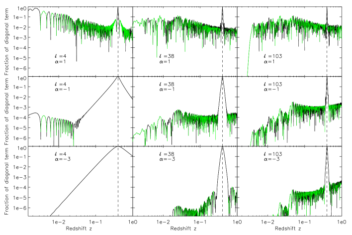
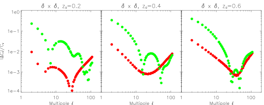
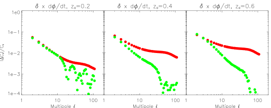
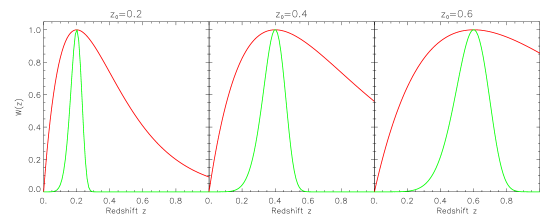
The Limber approximation is motivated by:
| (94) |
where the symbol denotes the Dirac delta function. Under the assumption that the spherical Bessel functions are rapidly oscillating for high enough -s, then one can write an integral over a generic power spectrum as
| (95) | |||||
where the power spectrum is assumed, in a cosmological context, to be a power law times some transfer function , . If seen as a four dimensional matrix with indices running on , the deviation of from a diagonal matrix in the last two indices, may be viewed as a measure of the error introduced by the Limber approximation.
In Fig. 19 we examine for the case where we have fixed to be the comoving distance to and where varies on the X-axis. We consider three cases for the multipole number: ; and three cases for the spectral index: which may be thought of as , , and . We take and . For the sake of clarity, the elements of have been normalized by the maximum value of each row. Black points denote positive values and green ones negative entries. The diagonal term (at ) has been marked by a vertical dashed line. From the figure it is clear that the deviation from a diagonal matrix is more apparent at low multipoles, and for more negative values of . At higher , however, the width of the matrix shrinks around , making the Limber approximation more precise. The actual error on these multipoles is related to how the off-diagonal terms are weighted by the time dependent factors, and how their sum cancels within the integration range.
Fig. 19 presents the errors on and , at three different redshifts and for thin (green color) and thick (red color) redshift shells (these are displayed in the bottom panels). In all cases, for , the errors are below 3%. We find that for , the net resulting error is larger for thin redshift shells than thick ones. This is inverted for , where the contribution to the off-diagonal terms are smaller for thin shells. However errors remain always below the few-percent level. The amplitude of the errors are defined by: the actual width of the peak around ; the amplitude of the oscillating floor around the wings of the peak at ; and the actual width of the redshift integration range compared to the width of the peak at .