Applications of quark-hadron duality in structure function
Abstract
Inclusive electron-proton and electron-deuteron inelastic cross sections have been measured at Jefferson Lab (JLab) in the resonance region, at large Bjorken , up to 0.92, and four-momentum transfer squared up to 7.5 GeV2 in the experiment E00-116. These measurements are used to extend to larger and precision, quantitative, studies of the phenomenon of quark-hadron duality. Our analysis confirms, both globally and locally, the apparent “violation” of quark-hadron duality previously observed at a of 3.5 GeV2 when resonance data are compared to structure function data created from CTEQ6M and MRST2004 parton distribution functions (PDFs). More importantly, our new data show that this discrepancy saturates by 4 Gev2, becoming independent. This suggests only small violations of evolution by contributions from the higher-twist terms in the resonance region which is confirmed by our comparisons to ALEKHIN and ALLM97. We conclude that the unconstrained strength of the CTEQ6M and MRST2004 PDFs at large is the major source of the disagreement between data and these parameterizations in the kinematic regime we study and that, in view of quark-hadron duality, properly averaged resonance region data could be used in global QCD fits to reduce PDF uncertainties at large .
pacs:
25.30.Fj, 24.85.+pI Introduction
To understand how Quantum ChromoDynamics (QCD) works remains one of the great challenges in nuclear physics today. The challenge arises from the fact that the degrees of freedom observed in nature, hadrons and nuclei, are not the same as the ones appearing in the QCD Lagrangian, quarks and gluons. The challenge is then to formulate a connection between the description of hard, or short-distance, scattering processes which can be calculated perturbatively in terms of quark and gluon degrees of freedom and their weak couplings, and soft, or long-distance, scattering processes, where the physical asymptotic states are prominent and the quarks and gluons interact strongly.
Given these strong quark-gluon interactions, or the large value of the strong coupling constant , the spectra of the asymptotic hadron states are not calculable within a perturbative QCD (pQCD) framework, and are difficult to directly connect to the underlying quark-gluon or parton dynamics. Yet, several instances exist in nature where the behavior of low-energy scattering cross sections, averaged over appropriate energy intervals, closely coincide with asymptotically high-energy scattering cross sections, calculated in terms of quark-gluon degrees of freedom. This phenomenon is referred to as quark-hadron duality, and may be a general property of quantum field theories with inherent weak and strong coupling limits, with QCD as a prime example.
The observation of a non-trivial relationship between inclusive electron–nucleon scattering cross sections at low energy, in the region dominated by the nucleon resonances, and that in the deep inelastic scaling regime at high energy predates QCD itself. While analyzing the data from the early deep inelastic scattering experiments at SLAC, Bloom and Gilman observed [1, 2] that the inclusive structure function at low hadronic final state mass, , generally follows a global scaling curve which describes high- data, and to which the resonance structure function averages. Following the development of QCD in the early 1970s, Bloom–Gilman duality was reformulated in terms of an operator product (twist) expansion of moments of the structure functions [3, 4]. This allowed a systematic classification of terms responsible for duality and its violations in terms of so-called higher-twist operators which describe long-range interactions between quarks and gluons. However, this description could not explain why particular multi-parton correlations were suppressed, and how the physics of resonances gave way to scaling [5].
Since then, with the development of high luminosity beams at modern accelerator facilities such as JLab, a wealth of new information on structure functions, with unprecedented accuracy and over a wide range of kinematics, has become available. One of the striking findings of the new JLab data [6, 7, 5] is that Bloom-Gilman duality appears to work exceedingly well, down to values as low as 1 GeV2 or even below. This is considerably lower than previously believed, and well into the region where is relatively large. Furthermore, the equivalence of the averaged resonance and scaling structure functions appeared to hold for each resonance, over restricted regions in , so that the resonance–scaling duality holds also locally. It was also found that quark-hadron duality manifests itself in the separated proton transverse () and longitudinal () structure functions.
The more recent JLab resonance structure function studies have revealed an important application of duality: if the workings of the resonance–deep inelastic interplay are sufficiently well understood, the region of high Bjorken- (, where is the longitudinal momentum fraction of the hadron carried by the parton in the infinite momentum frame) would become accessible to quantitative studies. This region remains largely unexplored experimentally due to the requirement of high-energy beams with sufficiently high luminosity.
The region is an important testing ground for nonperturbative and perturbative mechanisms underpinning valence quark dynamics, and is vital to map out if we hope to achieve a complete description of nucleon structure. Data from the nucleon resonance region, where quark-hadron duality has been established, could be used to better constrain QCD parameterizations of parton distribution functions (PDFs), from which also the hadronic backgrounds in high-energy collisions are computed [8]. The large- region also constitutes an appreciable amount of the moments of polarized and unpolarized structure functions, especially for the higher moments. It is precisely these moments that can be calculated from first principles in QCD on the lattice [9], in terms of matrix elements of local operators.
Note that, since the dependence of structure functions cannot be calculated on the lattice directly, one cannot easily use the lattice to learn about the degree to which duality holds locally. Indeed, the ability to calculate a leading-twist moment on the lattice implicitly uses quark-hadron duality to average the resonance contributions to a smooth, scaling function.
In this article, we quantitatively study the application of quark-hadron duality to access parton dynamics in the region of large , up to 0.9. For this, we accumulated a series of inclusive electron-proton and electron-deuteron scattering data in the nucleon resonance region ( 4 GeV2), at the highest momentum transfers accessible at JLab. These data are at values of far above where duality was quantitatively found to be valid in previous JLab experiments. The extracted structure function data are also compared with various state-of-the-art parameterizations of world data to improve our understanding of parton dynamics at large values of Bjorken .
The article is structured in five sections. Section 2 summarizes techniques of modeling the dynamics of the nucleon in terms of structure functions computed from PDFs and examines in detail few representative parameterizations of the nucleon structure function focusing on the large region. Section 3 is an overview of the experimental apparatus utilized to collect these experimental data and of the analysis steps taken to extract the cross section and the structure function. In Section 4 we present our studies of the application of quark-hadron duality to gain insight in the parton dynamics at large . In Section 5 we draw conclusions.
II parameterizations at large Bjorken
The purpose of this Section is to give an overview of the techniques typically employed to map out the dynamics of the nucleon via structure functions. This discussion points out the importance, but also the difficulty, of obtaining a parameterization of the structure function for the entire kinematic range. In particular, the exclusion of data in regions where the perturbative QCD mechanisms are not the only ones expected to contribute, greatly limits the applicability of these parameterizations and also our knowledge of the nucleon structure. In this context, quark-hadron duality might be the tool which could open kinematic regions not easily accessible otherwise to detailed studies. Four representative parameterizations will be examined in detail with an emphasis on the large region: ALLM97 [10], CTEQ6M [11], MRST2004 [12] and ALEKHIN [13, 14]. These parameterizations were used in our duality studies which will be presented in Sect. 4.
Lastly, the parameterization of the structure function from Bourrely et al. [15] will also be considered. This parameterization is obtained from parton distribution functions constructed in a statistical physical picture of the nucleon, where the nucleon is viewed as a gas of massless partons (quarks, antiquarks and gluons) in equilibrium at a given temperature in a finite size volume. The dependence of the parton distributions is chosen to correspond to a Fermi-Dirac distribution for quarks and antiquarks, and to a Bose-Einstein distribution for gluons. The parameterization involves a total of eight free parameters which are constrained by fitting high data from various experiments: NMC, BCDMS, E665, ZEUS, CCFR. A comparison of from Bourrely et al. to results from CTEQ6M and ALLM97 will be shown in Sect. 4.
Empirical Parameterization of : ALLM97. ALLM97, proposed as an update of ALLM [16] published in 1991, is a Regge motivated parameterization extended to the large regime in a way compatible with QCD expectations. The data set used to obtain the ALLM97 fit coefficients included all p measurements published up to 1997, with 3 GeV2, and covering a wide range in , 0 5000 GeV2 . The ALLM97 fit function has a total of 23 parameters, half of which are needed for the description of the low (high ) region where higher-twist terms are expected to be important. There are two important aspects to be noted in relation to the behavior of the ALLM97 parameterization at large (see Figs. 1 and 2).
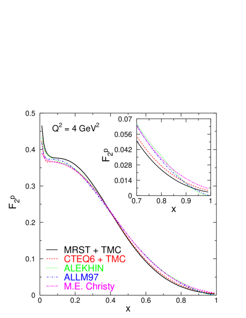
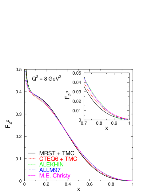
On one hand, the data set used to obtain the fit coefficients is selected with a rather low cut. Thus, it is expected that, if duality holds globally, the extrapolation of ALLM97 below of 3 GeV2 in the resonance region will work reasonably well, on average. On the other hand, ALLM97 being an empirical fit, some of its shortcomings like unconstrained and dependence or inability to fully account for target mass effects will become obvious as we probe kinematic regimes outside its domain of applicability. This will most likely be revealed in a clear manner when extrapolating to low regions.
QCD Parameterization of . Starting from two basic ideas of pQCD, factorization and evolution, the structure function can be calculated from PDFs extracted from hard-scattering data [18]. The theorem of factorization of long-distance from short-distance dependence in deep inelastic scattering (DIS) allows for the structure function to be expressed as a generalization of the parton model results:
| (1) |
where i denotes a sum over all partons (quarks, antiquarks and gluons) inside the proton, are coefficient functions independent of the long-distance effects while are parton distributions sensitive to the nonperturbative, long-distance effects inside the proton [19]. The evolution, on the other hand, enables the systematic, perturbative computation of logarithmic scale-braking effects and ensures that measuring (,) is enough to predict not only (,) but also (,) for all , assuming that both and are large enough that a perturbative expansion in is still appropriate. This is typically done by using the DGLAP evolution equations to evolve the parton distributions:
| (2) |
where are the evolution kernels (splitting functions) given by a perturbative expansion in , beginning with the leading order (LO) but also calculable to higher orders, next-to-leading order (NLO) or next-to-next-leading order (NNLO). The kernels have the physical interpretation as probability densities of obtaining a parton of type i from one of type j carrying a fraction of the parent parton’s momentum.
Thus, the three basic quantities are the coefficient functions , the evolution kernels and the PDFs . Of these, the first two are computed perturbatively as power series in . The physical non-perturbative parton distributions are extracted by combining theory and experiment and performing QCD fits. In a typical QCD fitting procedure the dependence of the parton distributions is parameterized at some low scale, , where higher-order corrections in are expected to be negligible, and then a fixed order ( either LO or NLO or NNLO) DGLAP evolution is performed to specify the distributions at higher scales where data exist. A global fit to the data then determines the parameters of the input distributions. There is considerable freedom in choosing the parametric form of the parton distributions at scale [18]. The parameterization should be general enough to accommodate all possible . A typical choice is:
| (3) |
where is a smooth function of , and determines the small and large behavior, respectively, and are coefficients to be determined from fits to data.
When performing QCD fits, there are several conceptual difficulties to take into account. First of all, a QCD analysis of measurements involves the use of the gluon distribution which is, a priori, unknown. In fact, the gluon distribution is the most uncertain of the PDFs and is particularly ill-determined for 0.3, with uncertainties reaching 200% by = 0.5 [11]. This in turn translates in an uncertainty in the determination from QCD analysis of PDFs since there is a correlation between the hardness of the gluon and the magnitude of , the quantity which sets the scale for [20]. The measurements should be able to provide a precise value of since the gluon distribution does not enter into the evolution. However, the experimental uncertainties of are still larger than those of and discrepancies in extracting were observed between different experiments in the region of 0.4 [21].
Then, it should be pointed out that, a standard QCD analysis of PDFs does not take into account all residual effects arising, for example, from higher-order radiative corrections in or/and non-perturbative higher-twist corrections. In particular, the higher-twist terms are non-factorisable and process dependent and QCD has no rigorous prescription to account for it. As a result, most PDFs extractions are performed using safe kinematic cuts for data selection in order to exclude regions where higher-twist or/and higher-order corrections in play an important role. A typical set of cuts employed to select data for fitting is 2 GeV2 and 12 GeV2 (this type of cut rejects the whole resonance region). Limiting the data coverage to a particular range in and will result in a limitation in the coverage. For example, for a fixed , a cut of will limit the range to /( - + ). Considering that the dependence of the PDFs is parameterized empirically, as exemplified in Eq. 3, and that the parameterization coefficients are extracted from fits to data, these data selection cuts, though they make possible the extraction of PDFs without the complications specified above, yield to unconstrained strengths of the PDFs at large [11].
To date, the large experimental uncertainties in the large regime, when excluding the low data, prevent answers to basic questions as to why the quark distribution appears to be softer than the quark distribution. For the same reason, the / behavior at large , a critical test of the mechanism of spin-flavor symmetry breaking, is highly unconstrained. Furthermore, knowledge of PDFs at large is essential for determining high-energy cross sections at collider energies such as in search of new physics beyond the Standard Model, where structure information at large feeds down through perturbative evolution to lower and higher values of [5]. Thus, it is of paramount importance to decrease the uncertainties in the extraction of PDFs by deriving the parameterizations directly from data without resorting to theoretical assumptions alone for the extrapolation to 1.
Extending to larger at a finite means encountering the resonance region. An important consequence of duality is that the resonance and deep inelastic regions are deeply connected and properly averaged resonance region data could facilitate our understanding of the deep inelastic region. In some of the QCD analysis performed, the higher-twist terms have been extracted from data selected with a kinematic cut of 10 GeV2 [22, 23, 14]. However, it was shown in several analyses [24, 25] that only a relatively small higher-twist contribution consistent with the one obtained in Ref. [22, 23, 14] would be necessary to describe the entire structure function spectrum. Indeed, S. Liuti et al. analyzed resonance region data within a fixed- framework. This study found that the higher-twist contributions in the resonance region are similar to those from 10 GeV2, with the exception of region where the effects seem to be larger. This is in no way surprising if one thinks of it as a consequence of quark-hadron duality which ensures that, on average, higher-twists are small or cancel. As a consequence of duality, the wealth of resonance region data could be utilized to access the large region and constrain the PDFs in this regime. This approach, however, requires a very good understanding of the dependence of the data in these kinematic regions of and where the perturbative evolution is no more the only mechanism responsible for the behavior.
Figures 1 and 2 depict three pQCD parameterizations of the structure function at two values, 4 and 8 GeV2, with a zoom-in of the large- region. The CTEQ6M parameterization shown is a QCD fit to hard scattering and DIS data (BCDMS, NMC, CCFR, E605, CDF, H1, ZEUS, D0) with 4 GeV2 and 12.25 GeV2. The dependence of the PDFs is parameterized at a of 1.3 GeV2 and then the QCD evolution equations are utilized to evolve the distributions at higher Q2 in the NLO (and LO). The authors employed the twist-2 pQCD formalism so the kinematic cuts used for data selection were tested to ensure that the introduction of simple phenomenological higher twist terms would not improve significantly the quality of the fit. The CTEQ6M fit shown in Figs. 1 and 2 is obtained in the (modified minimal subtraction) factorization scheme. One of the main improvements over earlier CTEQ fits is the addition to the global set of data of new measurements (H1, ZEUS, D0) which provide better constraints on the PDFs, in general, and on the gluon distribution at large , the result being a harder gluon distribution in this region. The other noteworthy improvement is the full treatment of uncertainties of the PDFs and their physical predictions, using an eigenvector-basis approach.
The MRST2004 parameterization is a QCD fit to a wide set of deep inelastic and related hard scattering data (BCDMS, SLAC, NMC, CCFR, CDF, H1, ZEUS, HERA, D0) with 2 GeV2 and 12.5 GeV2. The dependence of the PDFs is parameterized at of 1 GeV2 and a fixed order, LO or NLO or NNLO, QCD evolution is performed to specify the distributions at larger where data exist. A global fit to the data then determines the parameters of the input distributions. Though the fits are performed in the standard scheme, the gluon distribution is parameterized in the DIS (deep-inelastic scattering) factorization scheme and then transformed to the scheme. Together with more precise calculations of the splitting functions up to NNLO, this is actually the main improvement over earlier MRST fits (MRST2001 [26]). Indeed, the NLO global analysis with this new gluon parameterization appears to work extremely well when compared to Tevatron jet data and is even better for the NNLO fit. This objective couldn’t be accomplished by previous MRST parameterizations.
Both CTEQ6M and MRST2004 are shown here with target mass corrections (TMC) included according to Ref. [27]. CTEQ6M has more strength at large than MRST2004. For most part, this discrepancy originates from the fact that the two groups use different functional forms for the parameterization of the non-perturbative input parton distributions and neither parameterization is constrained by measurements in the large regime.
The ALEKHIN parameterization shown in Figs. 1 and 2 is an update of an earlier parameterization [14], the significant improvement being the use of recent calculations of the exact NNLO evolution kernel. The data used were from SLAC, BCDMS, NMC, HERA, H1, ZEUS with kinematic cuts of 2.5 GeV2, 3.24 GeV2 and x 0.75. The model for the data description was based on pQCD with phenomenological parameterization of the twist-2 and higher-twist contributions to the structure functions. The analysis was performed in the scheme with the number of flavors fixed at 3. The twist-2 PDFs were parameterized at = 9 GeV2. The pQCD analysis was done up to NNLO. Given the rather low cut used to select the data set, ALEKHIN parameterization includes, besides the typical parameters of pQCD, parameters to account for the target mass and dynamical higher-twist effects. This is a novelty, considering the standard procedure of performing QCD fits. The higher-twist contributions to the structure function were parameterized in additive form:
| (4) |
where has contributions from the twist-2 terms with target mass corrections included according to Ref. [27] and the dynamical twist-4 term is parameterized in a model-independent way as a piece-linear function of . The use of the exact NNLO corrections made possible an improvement in the positivity of the gluon distributions extrapolated to small and : in this parameterization the gluon distributions are positive up to = 1 GeV2, i.e. throughout the kinematic region where the parton model proved to be applicable. Since the ALEKHIN parameterization is based on fits to data with lower than CTEQ6M and MRST2004, its PDFs are expected to be better constrained at large .
Parameterizations of F. The parameterizations discussed above provide parton distribution functions from which the nucleon structure function can be constructed in QCD frame-work. ALLM97 is a fit to just the nucleon (proton) structure function. In order to construct the structure function for a nucleon inside a nucleus substantial additional challenges need to be overcome. There are a host of well-documented issues in extracting nucleon structure functions from nuclear data, even from deuterium data (see, for instance [28, 29, 30, 31, 32]). At large in particular, the effects of Fermi motion, nuclear binding, the EMC effect, off-shell corrections, and the like are quite large, and must be taken into account. Since there is no consensus on how best to accomplish this, we have here chosen to compare the measured deuterium resonance region data directly to deep inelastic deuterium structure functions. Specifically, we have chosen to multiply the array of structure functions previously discussed by the following parameterization of d/p (deuteron over proton) [33]:
| (5) |
This equation is the result of a data fit up to = 0.8, and may not be constrained correctly at the highest . Moreover, it assumes no -dependence, a need for which has been indicated in other works [34]. A more thorough approach might in the future consider specifically structure functions formed from nuclear PDFs, such as those found in [35, 36, 37, 38].
Target Mass Corrections. At large enough values of and , QCD provides a rather clear and rigorous perturbative description of the physics that generates the behavior of the structure function. When , where is the proton mass, both the nonperturbative kinematical power corrections (target mass corrections) and the dynamical higher twist have to be taken into account. Since these characterize the long-range non-perturbative interactions between quarks and gluons, the dynamical higher-twist terms contain information about the dynamics of confinement. The target mass corrections, on the other hand, arise from purely kinematic effects associated with finite values of / = /. The target mass terms are related to the twist-2 operators and contain no additional information on the non-perturbative multi-parton correlations. In consequence, target mass effects should either be corrected for in the data or the effect should be included in the QCD fits if one aims for a consistent comparison of data to QCD fits. The target mass effects were taken into account in the CTEQ6M, MRST2004 and ALEKHIN parameterizations of the structure function according to the prescription of Georgi and Politzer [27]. It is non-trivial to note that there is not an universally agreed-upon prescription to account for target mass [39, 40, 41], and so the choice of approach inherently introduces some uncertainty to this analysis.
III Experiment and Data Analysis
The experiment E00-116 was carried out in Summer 2003 in Hall C, at JLab. A fixed electron beam of energy 5.5 GeV came incident on cryogenic targets. The target system consisted of 4 cm long liquid hydrogen and deuterium, contained in circular aluminum cans. Scattered electrons were detected in the High Momentum Spectrometer (HMS). The Short Orbit Spectrometer (SOS) was used for detection of positrons, which was used to estimate possible electron background originating from charge-symmetric processes such as production and subsequent decay in the target. The data were taken at various scattering angles and momenta as follows: for each fixed spectrometer angle, the central momentum was varied in order to cover a region in from about 1.2 to 4.5 GeV2. The kinematics covered by this experiment are shown in Table 1. These data extend the existing Hall C resonance region measurements at larger and [6, 7].
| Angle(deg) | Momentum(GeV/) | ((GeV)2) | |
|---|---|---|---|
| 2.26 | |||
| 37.93 | 1.94 | 0.48-0.92 | 3.58-5.48 |
| 1.67 | |||
| 2.17 | |||
| 41 | 1.86 | 0.53-0.94 | 3.99-5.86 |
| 1.60 | |||
| 1.94 | |||
| 45 | 1.67 | 0.55-0.95 | 4.28-6.29 |
| 1.44 | |||
| 1.34 | |||
| 55 | 1.16 | 0.60-0.94 | 5.01-7.07 |
| 1.47 | |||
| 1.31 | |||
| 60 | 1.19 | 0.52-0.95 | 4.52-7.38 |
| 1.04 | |||
| 0.89 | |||
| 70 | 0.91 | 0.60-0.83 | 5.38-7.11 |
| 0.80 |
III.1 Experimental Setup
III.1.1 Beam Line
During E00-116, the Continuous Electron Beam Accelerator Facility (CEBAF) at JLab provided an unpolarized, Continuous Wave (CW) electron beam of 5.5 GeV, with currents up to 100 A. The beam was steered from the Beam Switch Yard to the experimental hall through the beam line. Hall C beam line is equipped with magnets used to focus and steer the beam, as well as several monitors needed to measure the energy, current, position and profile of the beam. The profile and the absolute position of the beam is monitored utilizing superharps. A superharp consists of a frame and three tungsten wires (two horizontal and one vertical) which are moved back and forth through the beam to determine the centroid position to about 10 m. However, the superharp cannot be used during the data taking because it has a destructive interaction with the beam. Therefore, Beam Position Monitors (BPMs) [42] are used to continuously monitor the relative beam position during data taking. The BPMs are nondestructive to the beam and are calibrated with superharp scans. During this experiment, the typical relative variation of the beam position at the target was found to be less than 0.2 mm.
The beam energy is measured using the superharps and the dipole magnets in the beam line. Due to the fact that the dipole fields are accurately mapped and that the beam path is determined with high precision by the superharps, the accuracy of the absolute beam energy measurement is at the level of 5 10-4 GeV.
The beam current and charge in Hall C is measured by a system of beam current monitors (BCMs) together with a parametric current transformer (Unser) [43]. All these monitors are placed in the beam line before the target in the following order: BCM1, Unser, BCM2 and BCM3. Although the BCMs have a very stable offset, the gain drifts with time and the Unser is used for BCMs gain calibrations. Dedicated calibration runs are typically performed to minimize the effects of drifts in the BCMs gains. For this experiment, BCM2 was used for monitoring but due to time constraints, no BCM calibration runs were taken. However, the experiment that ran just before E00-116 had the same set-point for the BCM2 gain, such that it was possible to use their calibration runs taken 5 weeks and 1 week before this experiment [44].
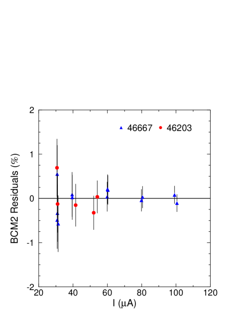
The difference in BCM2 gain and offset when using each run individually or the combined runs was below 0.1%, indicating that there were no significant drifts in the BCM2 gain over a month period. Figure 3 shows that the difference between the current as given by the BCM2 after calibration and the current as given by the Unser (the residuals) are within 0.15% above 50 A. The calibration result from the combined runs was used to calculate the current and the charge for this experiment. For this experiment current regime, the normalization uncertainty in the current measurement was estimated to be 0.3% at 100 A and originated from possible small drifts of the BCM gain, from the precision of the BCM calibration and from the accuracy of the Unser in measuring the current, the latter bringing the largest contribution. The point-to-point uncertainty was estimated to be 0.05% by taking the difference in the normalization uncertainties propagated at 80 A and 100 A, this being roughly the range in the beam current used in this experiment.
The electron beam generated by CEBAF is a high current beam with a very small transverse size (100-200 m FWHM). To prevent damage to the targets and to minimize the changes in the cryotarget densities due to localized boiling, a rastering system is used to distribute the deposited energy of the beam in an uniform manner over the target volume. The raster consists of two sets of steering magnets: the first set of magnets rasters the beam vertically and the second horizontally. For this experiment the raster consisted of a 22 mm uniform structure. A detailed description of the Hall C raster system is given in Ref. [45].
III.1.2 Target
This experiment used the standard liquid hydrogen and liquid deuterium cryogenic target system in Hall C. The liquid targets were contained in aluminum cans. Data were taken on aluminum foils (dummy target) for background measurement and subtraction. Also several runs were taken using a carbon foil target in order to determine the beam offsets relative to the pivot of the target. The cryogenic target cells were mounted on a cryostack together with the combination of carbon and aluminum target sled. The cryogenic system ensured that the temperature and density of the liquid targets were maintained during data taking at optimum values of 19 K and 0.0723 g/cm3 for hydrogen and 22 K and 0.1674 g/cm3 for deuterium.
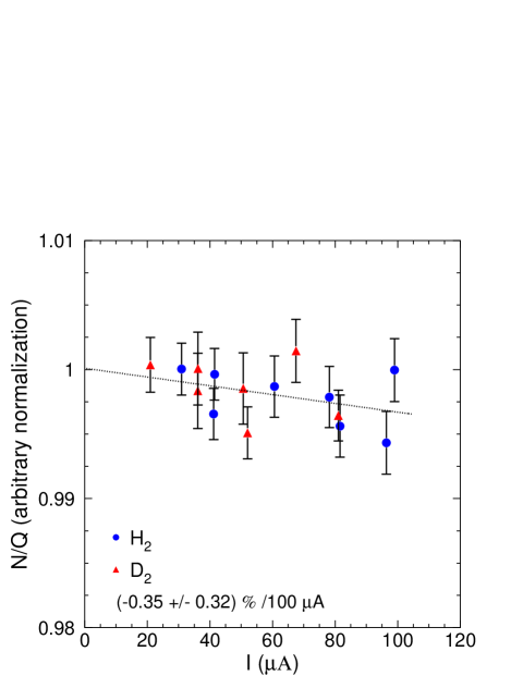
To accurately determine the experimental luminosity it is necessary to have a precise knowledge, among others, of the targets’ density and thickness. Though the cryogenic system is designed to ensure that the liquid hydrogen and deuterium targets are maintained at a fixed nominal temperature in all conditions, in reality, when the beam passes through the targets and deposits heat there are local changes in the temperature and density of the cryogen (boiling effect). Dedicated data (luminosity scans) are taken to study and correct for this effect. During E00-116, luminosity scans were performed on both hydrogen and deuterium targets. It was found that the boiling effect gives a small correction of (0.35 0.32)% / 100 A to the luminosity for both cryogenic targets as seen in Fig. 4. This parameterization was utilized on a run-by-run basis to correct for the boiling effect for both liquid targets. The majority of the data were collected at 100 A. The density correction at this current is of the size of the uncertainty of the fit, therefore the normalization uncertainty was taken to be 0.35%. The point-to-point systematic uncertainty on the density correction, originating from the uncertainty in the current, is negligible.
Because of the circular geometry of the cryogenic target cell, a careful analysis is required to determine the effective target length that will enter in the calculation of the luminosity. If the beam was exactly aligned along the diameter of the target, the effective target length will simply be the outer diameter of the target cell minus the cell walls. If there is a displacement between the beam and the center of the target, then the effective target length will be , where is the inner radius of the cell and is the beam offset from the center of the target. For E00-116, several sources of information were used to determine the effective target length: the target survey that provides measurements, at room temperature, of the outer diameter of the cell together with the thickness of the cell walls, a survey of the target position relative to the pivot, and dedicated data taken on a central Carbon foil that provide the beam offset relative to the pivot [46]. The effective target length used in the cross section extractions is listed in Table 2.
| Target | Effective Target Length(cm) |
|---|---|
| Hydrogen | 3.946 0.029 |
| Deuterium | 3.927 0.029 |
III.1.3 Spectrometers
In what follows, a summary of the main characteristics of Hall C spectrometers will be given with emphasis on the aspects relevant to E00-116. Detailed information about the Hall C HMS and SOS can be found in Ref. [47, 48]. The HMS is a magnetic spectrometer consisting of a 25 deg vertical bend dipole magnet for momentum dispersion and three quadrupole magnets for focusing. All magnets are superconducting. For this experiment, the HMS was operated in the point-to-point optical tune. The range used in the momentum () acceptance, = , was of 8% while the range in the angular () acceptance, was 35 mrad. The SOS consists of a quadrupole magnet and two dipole magnets. For E00-116, the point-to-point optical tune was used. The range used in was of (-15,+20)% while the range in the angular acceptance was 60 mrad.
The detector packages for the two spectrometers are very similar and consist of two drift chambers for track reconstruction, scintillators arrays for triggering, a threshold gas Cerenkov and an electromagnetic calorimeter, which were both used in this experiment for particle identification (PID) and pion rejection.


The HMS Cerenkov counter was used to distinguish between and with momenta between 0.8 and 2.3 GeV. For this purpose, the Cerenkov tank was filled with Perfluorobutane (, = 1.00143 at 1 atm and 300K) at about 0.9 atm making the detector fully sensitive to but insensitive to in the momentum range specified above. The SOS Cerenkov counter was used to detect and reject with momenta ranging from 0.8 to 1.7 GeV. The Cerenkov tank was filled with Freon-12 ( = 1.00108 at 1 atm) at about 1 atm giving a Cerenkov threshold of 3 GeV for and 11 MeV for . For E00-116, a typical spectrum of the HMS Cerenkov number of photoelectrons is shown in Fig. 5. In this distribution, the events peak at zero while the events give an average of about 13 photoelectrons.
The HMS and SOS calorimeters are identical except for their size. Each calorimeter consists of 10 cm 10 cm 70 cm blocks of TF-1-1000 type lead glass ( = 3.86 g/cm3, = 1.67 and radiation length r.l. = 2.5 cm). The HMS calorimeter is 13 blocks high while the one in the SOS just 11. The calorimeters are rotated by 5 deg from the spectrometers optical axis in order to reduce eventual losses through the cracks between the blocks. For this experiment, the calorimeters were used to detect (HMS) and (SOS). The hadrons that could have reached the calorimeters were mostly or . The () were distinguished from () according to their fractional energy, total energy deposited in the calorimeter, normalized by the momentum. The () deposit their entire energy in the detector peaking in the fractional energy spectrum at 1; the () deposit around 0.3 GeV and they will peak in the fractional energy distribution at 0.3 GeV/. A typical distribution of the fractional energy deposited in the HMS calorimeter is shown in Fig. 6.
III.2 Data Analysis
The inclusive electroproduction cross section can be expressed as:
| (6) |
Here, is the number of incident electrons and is the number of target particles per unit area, which can be calculated in terms of the mass density , the atomic number A and the thickness from ( is Avogadro’s number). is the number of scattered electrons in the solid angle and in the energy range . is the background, is the detector acceptance and is the detector efficiency. The most significant corrections that were applied to will be discussed below.
III.2.1 PID Cut Efficiency
The rejection of negatively charged pions was accomplished by placing requirements on both the number of photoelectrons collected by the Cerenkov detector, number of photoelectrons larger than 2, and the fractional energy deposited by the particle in the calorimeter, fractional energy larger than 0.7. In what follows, the efficiency of these cuts in not rejecting valid electrons will be discussed.
Cerenkov Cut Efficiency. In order to determine how many electrons are lost when applying the Cerenkov cut number of photoelectrons larger than 2, it is important to work with a clean sample of electrons (no pion contamination). Once a clean sample of electrons is selected, than the Cerenkov cut efficiency is determined from the ratio of number of events that pass the cut to the total number of events in the clean sample. If the sample is pion contaminated then the Cerenkov cut efficiency will be artificially lower. Unfortunately, it was impossible for this experiment to select a clean sample of electrons just with a calorimeter cut. For the particular kinematics of E00-116, the pion to electron ratio was rather large (up to 150:1). The pions can undergo charge-exchange reactions and deposit up to their entire energy in the calorimeter. This could result in a high-energy tail for pions which could extend beyond 1 in the fractional energy spectrum making the selection of a clean sample of electrons practically impossible even with high calorimeter cuts. The unbiased electron cut efficiency for the Cerenkov was determined by extrapolating to zero pion to electron ratio. It was found to be (99.60 0.24)%, which in very good agreement with the findings of other experiments that ran at similar conditions [49]. This value was used as a correction for the data. The normalization systematic uncertainty was taken to be the uncertainty of the fit extrapolation at zero pion to electron ratio, 0.24%.
Calorimeter Cut Efficiency. Just as for the Cerenkov, the estimation of how many valid electrons are lost when using a cut on the fractional energy deposited in the calorimeter was complicated by the fact that, for this experiment, the large pion to electron ratio made impossible the selection of a clean sample of electrons using just a cut on the number of photoelectrons acquired in the Cerenkov detector. The same approach was taken in this case as for the estimation of the Cerenkov cut efficiency: the calorimeter cut efficiency was extrapolated to zero pion to electron ratio in order to find the true electron efficiency. The extrapolation was done for each momentum setting separately in order to deconvolute the efficiency dependence on the pion to electron ratio from the dependence on the resolution of the calorimeter. An example of the efficiency extrapolation at zero pion to electron ratio for one momentum setting is shown in Fig. 7.
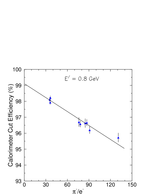
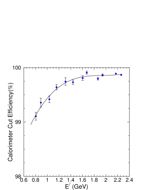
The efficiency, obtained in this manner, and parameterized as a function of momentum is shown in Fig. 8. The parameterization was used as a correction in the data analysis. Our parameterization was compared to the result obtained from an experiment that ran in similar experimental conditions but at different kinematics where the pion to electron ratio is small [49]. The two results were found to agree within 0.3%. The normalization and point-to-point uncertainties on this correction were estimated to be 0.3% and 0.25%, respectively.
III.2.2 Backgrounds
There are three physical processes that are possible sources of background for this experiment: electrons scattered from the target aluminum walls, negatively charged pions that are not rejected by the PID cuts, and electrons originating from other processes like charge symmetric processes which produce equal number of positrons. Each of these possible sources of background will be discussed in what follows.
Target Cell Background. During data taking on the cryogenic targets, some of the incoming electrons scatter on the aluminum walls of the target cell and end up being detected at the same kinematics as the electrons that scatter from the cryogen. This background has to be determined and subtracted from the measured yields in order to obtain the yields for scattering from the cryogen only. To determine this background dedicated data were taken on a dummy target at exactly the same kinematics as on hydrogen and deuterium. In order to minimize the data acquisition time, the total thickness of the dummy target was about eight times the total cell wall thickness seen by the beam. The background coming from the scattering from the target cell walls , was determined as:
| (7) |
where is the spectrometer angle, is the total charge incident on the cell walls (dummy), is the total thickness of the cell walls (dummy), (, ) is the number of events collected from the dummy run after applying efficiencies and dead time corrections and is the external radiative correction (external bremsstrahlung emission) for the cell walls (dummy). The target cell background subtraction was performed for each hydrogen and deuterium run on a (,) bin-by-bin basis. The size of this background was at most 18% and its uncertainty was dominated by the statistical uncertainty on and by the uncertainty in measuring the thickness of the cell walls and dummy. The thickness of the cell walls was known up to 1% while, by comparison, the uncertainty in the dummy thickness measurement was negligible [50]. This led to a systematic uncertainty in the cross section of at most 0.2%. The statistical uncertainty on was propagated to the uncertainty of the cross section.
Pion Background. Even after applying the PID cuts, some pion background may still be present. Although pions do not produce Cerenkov light directly, they can generate, through ionization, -rays in the materials preceding the Cerenkov detector (electron knockout). These knock-on electrons could have high enough energy to emit Cerenkov light and pass the PID Cerenkov cut. In the electromagnetic calorimeter, the pions give signal according to their energy loss but through a charge-exchange reaction they can produce neutral pions which decay into or . In this way, the entire energy of the pion can be deposited in the calorimeter. This process typically gives the high-energy “tail” for pions that extends to deposited fractional energy of 1.
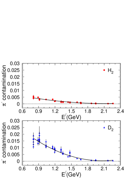
For this experiment, the pion background was estimated using a method developed for the Hall C E99-118 analysis [34] in which the pion rejection factor is used to normalize the pion fractional energy distribution in the calorimeter. The number of events in this normalized distribution that pass the PID calorimeter cut of 0.7 represents the pion contamination. The result of the pion contamination estimation for this experiment is shown in Fig. 9 for both hydrogen and deuterium targets. As expected for a heavier target, the pion contamination for deuterium (maximum of about 1.7%) is about 3 times larger than for hydrogen (maximum of 0.5%) at the lowest momentum. For this background subtraction, parameterizations as a function of momentum were used as corrections (no angle dependence was observed). The point-to-point uncertainty on this correction was determined to be 0.2% for both targets.
Charge-Symmetric Background. For electron-proton scattering there is a significant probability to produce a neutral pion in the target which then decays into or . The photons can further convert into electron-positron pairs in the target material or in the materials preceding the detectors. Photons can also be produced through the Bethe-Heitler process. However, the leptons resulting from Bethe-Heitler processes are very forward peaked so their contribution is significant only at forward angles. The outcome is that the secondary electrons will end up being detected together with the scattered electrons. For the kinematics of this experiment (backward angles) the dominant source of secondary electrons is the neutral pion production in the target and the subsequent decays. The electron production through Bethe-Heitler process is negligible. The fact that the background electrons are produced in pairs with positrons (charge-symmetric background) can be exploited experimentally and the background electrons can be disentangled from the scattered electrons by detecting positrons.
For E00-116, due to the limited running period (less than a week), it was decided to take advantage of the availability of the SOS. The SOS has a larger momentum acceptance than the HMS and two SOS momentum settings could easily cover an HMS scan with three momentum settings. However, by using a different spectrometer for positron measurements the photon to electron-positron pairs conversion factor is different as the photons encounter different radiation lengths of material. In addition, the SOS acceptance function and the detector inefficiencies are different than the HMS ones. Taking into account these considerations, we decided that an accurate estimation of the charge-symmetric background would require the extraction of the positron cross sections rather than the yields as it was done for previous Hall C experiments. This way, the charge-symmetric background would be corrected by subtracting the measured positron cross section from the measured electron cross section bin-by-bin on a (,) grid.
The first step in the positron cross section analysis was to perform the detectors calibrations. Once the calibrations were performed, the positron yield selected with PID cuts was binned in the (,) acceptance around the central values. The yield was corrected for the electronic and computer dead times and for the tracking inefficiency. In order to obtain the positron yields from the cryotargets alone, the endcap contributions had to be subtracted. Also the pion contamination was determined and parameterized as a function of momentum for each cryotarget and applied as correction to the yield. Next, the spectrometer acceptance corrections were calculated and applied to the yield. Thus, the positron cross section was obtained on a (,) grid.
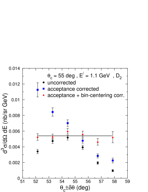
Our goal was to determine the cross section at the central angle as a function of momentum but still to keep the statistics accumulated. This could be done, in principle, by statistically averaging the measured cross section over the angular acceptance. However, the variation of the positron cross section across acceptance was non-negligible. Therefore, before averaging, a model was needed to remove the cross section dependence (the so called bin-centering correction). The positron cross section model used for this purpose was developed by P. Bosted [51]. The model uses a fit to the charged pion production data accumulated at SLAC [52]. The neutral pion production is estimated as the average of the positive and negative pion production. The positron cross section is calculated using the decay branching ratios for a neutral pion and the radiation length of the material where a photon that results from the decay can produce electron-positron pairs. Taking into account that the positron cross section model described above was used just for bin-centering, the main requirement was that the model should describe the shape of the angular dependence of the positron cross section. To make sure that this requirement was met, first it was checked if, after applying the bin-centering correction, there is any angular dependence left across the acceptance. A typical example is shown in Fig. 10 where it can be seen that, within the statistical uncertainty, the bin-centering correction removes the angular dependence of the cross section.
It was also checked that the data overlap in the angular acceptance from one central angle setting to the next if the model would be used to center the data at certain angle values in the acceptance. Good agreement was found for neighboring scans in the overlapping region.
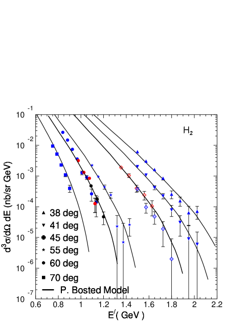
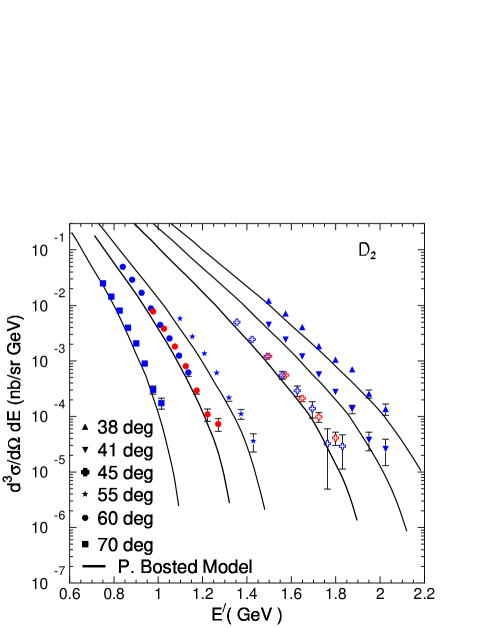
Finally, the positron cross section was extracted at fixed central angles as a function of momentum. Figures 11 and 12 show the positron cross section for both hydrogen and deuterium targets compared to the model of P. Bosted. It can be seen that the model describes qualitatively well the momentum dependence of the cross section.
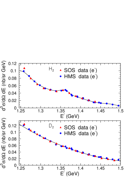
As stated previously, the electron data, both the scattered and the background electrons, were taken using HMS while the charge-symmetric background was measured using SOS. Therefore, at the end of the experiment, a setting was taken at the same kinematics in HMS and SOS (both spectrometers were set on negative polarity). The result of the analysis of this scan in the two spectrometers is shown in Fig. 13. It was found that the analysis in the two spectrometers agreed within 1.3%. This translated in a normalization uncertainty in the scattered electron cross section below 0.2%, considering that the relative contribution of the charge symmetric background to the measured cross section was at most 15%.
In the end, the charge symmetric background was subtracted bin-by-bin in (,). For the subtraction, the positron cross section had to be centered at the scattered electron data kinematics. The model of P. Bosted was used for this purpose. Quantitatively, it was found that the use of the model for bin-centering corrections in momentum introduced an uncertainty of 6% in the positron cross section at 38 deg, 41 deg, 45 deg, 55 deg and of 20% at 60 deg and 70 deg. This translated in an uncertainty on the electron cross section up to 2% at the lowest momentum at 60 deg and 70 deg, but below 0.2% for the rest of the data.
III.2.3 Acceptance Corrections
For a fixed angle and momentum setting, the spectrometers have a finite angle and momentum acceptance. This experiment used the same procedure of extracting the spectrometer’s acceptance functions as previous Hall C experiments. This procedure is described in detail elsewhere [53].
For this analysis, the acceptance correction was applied on a bin-by-bin basis in (,). The point-to-point uncertainty on the acceptance correction in HMS was estimated to be 0.8%. This is dominated by the position uncertainties on the target, collimator, magnets, and detector package. The normalization uncertainty on the acceptance correction was determined by combining in quadrature an uncertainty of 0.7% coming from the reduction in the solid angle and an uncertainty of 0.4% due to modeling of the HMS optics [53].
III.3 Cross Sections Extraction
For this experiment, the electroproduction differential cross section and was extracted according to Eq. 6, binned in 16 and 20 bins in momentum and angle, respectively. Our goal was to obtain the one photon-exchange (Born) cross section at a fixed angle as a function of momentum. For this, two additional corrections were necessary: the bin-centering correction, which makes possible the extraction of the differential cross section at a fixed angle without sacrificing statistics and the radiative corrections which are necessary to obtain from the measured cross section the one photon-exchange contribution. Considering that both the bin-centering corrections and the radiative corrections are calculated using a model for the cross section, the sensitivity of our results to the model input was studied in detail. All this will be discussed in what follows.
Bin-Centering Corrections. As previously mentioned, the measured cross section was initially extracted binned in small momentum and angle bins corresponding to the acceptance intervals in and , respectively. The goal, however, was to extract the cross section at a fixed angle, the central angle , keeping all the statistics accumulated. If the cross section would not vary across the acceptance, then the cross section at could be simply obtained by statistically averaging the cross section over the angular acceptance. However, for the kinematics of this experiment, the variation of the cross section over the angular acceptance was not negligible. Thus, before statistically averaging, the so called bin-centering correction had to be applied in order to center the cross section measured in the acceptance interval at . This correction was applied as:
| (8) |
where and are the model cross sections calculated at and , while and are the cross sections extracted from the data at and . The bin-centering correction was applied to the measured radiated hydrogen and deuterium cross sections using the radiated model cross section. The models used to calculate the correction will be discussed next.
Radiative Corrections. In the perturbative picture, the lowest order process in (the electromagnetic running coupling constant) that contributes to the cross section for inclusive electron-nucleon scattering is represented schematically in Fig. 14 (a). Besides this leading one photon exchange diagram (Born), there are higher order processes in that contribute to the scattering. These diagrams are shown schematically in Fig. 14 (b, c, d, e) and include vacuum polarization (the exchanged photon creates particle-antiparticle pairs), vertex processes (emission and reabsorption of virtual photons), and Bremsstrahlung (emission of real photons in the field of the nucleon during interaction). In order to determine the differential cross section that accounts just for the one photon exchange process, all the other contributions from higher order processes in have to be calculated and corrected for in the measured cross section.

The radiative processes can be divided into two main categories: internal and external. The internal effects take place at the scattering vertex and include Bremsstrahlung, vacuum polarization, vertex processes and multiple photon exchange. External Bremsstrahlung occurs within the target material before or after the primary scattering takes place and is dependent on the target thickness. As a consequence, the energy of the incoming and/or the scattered electron will change.

The measured cross section can be written as the sum of various processes (Fig. 15):
| (9) |
| (10) |
To obtain the Born inelastic cross section, the radiative tails from elastic/nuclear elastic and quasielastic cross sections were subtracted while the inelastic radiative effects were corrected multiplicatively. In practice, the usual calculation of radiative corrections includes only the emission of one hard photon. However, there is a probability for the electron to emit two hard photons. Therefore additional corrections (the term) should be taken into account when estimating the radiative correction.
There are two programs utilized for the radiative corrections calculations: one based on the Mo and Tsai formalism [54] and the other one based on the Bardin formalism [55], which includes in the calculations the two hard-photon radiation and has a different treatment of the soft photon contribution. The program based on Mo and Tsai formalism calculates both internal and external radiative corrections, unlike the Bardin one which calculates just internal radiative corrections. For this experiment, the radiative corrections (both internal and external) were estimated using the Mo and Tsai formalism. The term correction was estimated using the Bardin formalism and at this experiment kinematics it proved to be below 0.5 (1) for hydrogen (deuterium). The size of the correction is within the theoretical uncertainty of the calculation and it was assigned as a point-to-point uncertainty.
Additional uncertainties in the experimental cross section originate from the elastic (elastic and quasielastic) contribution subtractions. At the kinematics of this experiment, the elastic contribution to the total experimental cross section is negligible. The uncertainty coming from the quasielastic contribution subtraction was estimated by propagating the point-to-point model uncertainty into the experimental cross section. This kinematic dependent uncertainty was parametrized for each angle setting separately. Finally, the normalization uncertainty in the cross section coming from the theoretical uncertainty in the radiative corrections calculation was estimated to be 1 [56].
Iteration Procedure As stated previously, the bin-centering corrections were calculated using a model for the cross section. The same model was typically used to calculate the radiative corrections. In order to minimize the model dependence of the extracted cross section, an iterative procedure was followed. First, a starting model was used to calculate both the bin-centering and radiative corrections. Then, the extracted cross section was fit and the new fit was used to calculate the corrections and reextract the cross section. This process continued until the extracted cross section did not vary significantly (not more than 0.3%) from one iteration to the next. Additionally, the iteration procedure was followed using two different starting models. After the last iteration, the two sets of cross sections were expected to be consistent.
For the two starting models (fits to previous data) used were the model of M.E. Christy and P. Bosted [57] and model [58]. The fitting procedure used is described extensively in Ref. [57]. Only two iterations were necessary and it was found that the difference in the cross section between the last iteration and the one before last was about 0.3%. Also after each iteration the difference in the cross section when starting with the two models specified above was calculated. This difference after the last iteration was assigned as a kinematic dependent uncertainty accounting for the model dependence of the final result.
For measurements, the iteration was performed using the same fitting procedure as for but with one modification: the fit form for the resonances used non-relativistic Breit-Wigners. The data seemed to be described better around pion threshold by such a fit. Three iterations were performed and the difference in the cross sections between the last iteration and the second last was around 0.3%. Just like for the data set, two different models were used in the iteration procedure: the Bodek model [59] and ALLM97 [10] multiplied by the parameterization of the ratio of the deuterium and the proton electroproduction cross sections [33]. The difference between the two sets of cross sections after the last iteration was parameterized to give the uncertainty originating in the possible model dependence of the final result.
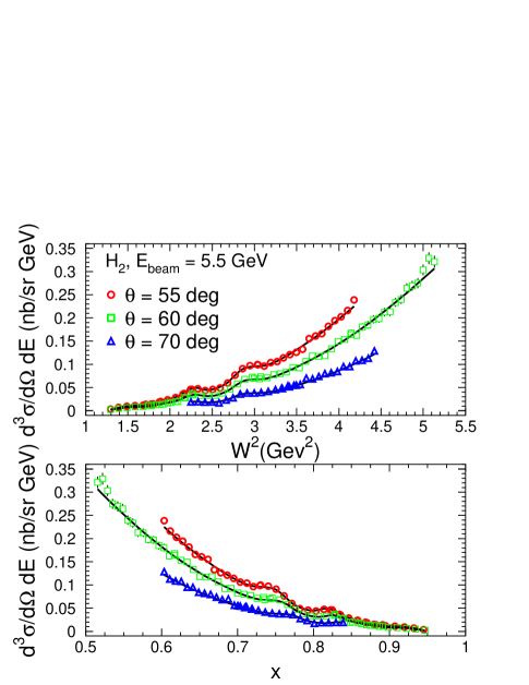
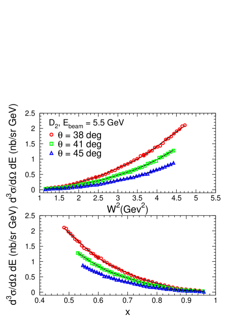
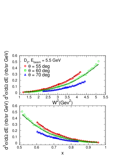
Systematic Uncertainties The total point-to-point systematic uncertainty in the cross section extraction was taken as the sum in quadrature of the individual uncertainties. An overview of these uncertainties is given in Table 3. The total normalization systematic uncertainty amounted to about 1.75% while the statistical uncertainty is below 3%.
| Quantity | Uncertainty | () |
|---|---|---|
| Beam Energy | 5x | 0.30 |
| Scattered Energy | 5x | 0.25 |
| Scattered Angle | 0.2 mrad | 0.26 |
| Beam Charge | 0.05 | 0.05 |
| Dead time | 0.25 | 0.25 |
| Trigger Efficiency | 0.2 | 0.2 |
| Tracking Efficiency | 0.2 | 0.2 |
| PID cut efficiency | 0.25 | 0.25 |
| Pion Cont. Subtraction | 0.2 | 0.2 |
| Charge-Symmetric Background | 6 - 20 | 2 |
| Acceptance Correction | 0.8 | 0.8 |
| Radiative Corrections | 0.5-3.6 | 0.5-3.6 |
| Model dependence | 0.2-5 | 0.2-5 |
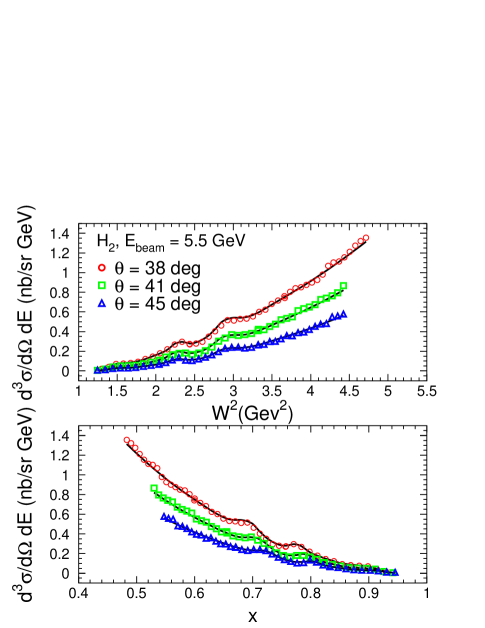
The total and Born deradiated differential cross sections extracted from this experiment for both and , together with the point-to-point associated uncertainties are given in Tables 5-9. The extracted Born differential cross sections are also shown as a function of and in Figs. 16-19. These data provide large and intermediate high-precision measurements in the resonance region where the precision of existing data from SLAC is typically 5 to 30% for the statistical uncertainty alone. This precision is not enough to distinguish between theoretical parameterizations of the structure function which at a of 8 GeV2 and = 0.8, for example, differ by at most 30% as shown in Fig. 2.
III.4 Extraction
The structure function was calculated utilizing the formula:
| (11) |
where , and is the electromagnetic coupling constant. The quantity is the degree of polarization of the virtual photon:
| (12) |
and is the flux of the virtual photon:
| (13) |
The extraction of requires the knowledge of both the differential cross section and the quantity which is the ratio of the longitudinal to the transverse component of the cross section. For this experiment, it was not planned to measure but just the differential cross section since is not expected to be large in the range of this data set. Thus, for the structure function extraction, it was needed to resort to an existing parameterization. In order to estimate the sensitivity of the structure function to different parameterization, the following approach was taken. was extracted at the lowest and highest for this experiment using three different parameterizations: R from R1990 [60], R1998 [61] and E94-110 [56], respectively. It was found that varies on average by 2% when different parameterizations are used. R1990 and R1998 are parameterizations of extracted mainly from DIS measurements, while from E94-110 is extracted from resonance region measurements, only. The parameterization from E94-110 is kinematically limited to 3.85 GeV2 and typically lower than this experiment. However, it was shown to agree, where applicable kinematically, to R1990 and R1998. The parameterization R1998 was obtained using a larger data set than R1990 (R1998 used, in addition to the data set of R1990, other measurements extending the parameterization to lower and higher ), and also had a better confidence level of the fit (73%) than R1990 (61%). For all these reasons, from R1998 was used for the structure function calculation and an additional uncertainty of 2% was assigned to in order to account for the sensitivity of the extraction to .
IV Results
In this section we present our results with a preamble of previous quark-hadron duality studies. With this very brief summary of previous studies we intend to create the apropriate context for the detailed discusssion of our results and the conclusions that will be drawn.
IV.1 Previous Quark-Hadron Duality Studies with Electron Scattering
Over three decades ago, Bloom and Gilman acknowledged the resonance-scaling connection in inclusive electron-nucleon scattering. After more than 20 years, it was an early JLab experiment that revived the interest in the phenomenon of quark-hadron duality [62, 6, 63]. This experiment confirmed the observations of Bloom and Gilman and, in addition, acknowledged the onset of duality also locally. The findings of these studies prompted interest in a more detailed analysis of duality, one within the QCD formalism.
Comparisons of the resonance region data to some QCD predictions were performed using measurements from JLab experiment E94-110 [56, 7]. The and extracted from E94-110 were compared to QCD fits from the MRST [65] and CTEQ6 [66] collaborations evaluated at the same as the data and with the inclusion of target mass corrections. It was observed that the QCD fits seem to describe on average the resonance strength at each value investigated - of 1.5, 2.5 and 3.5 GeV2- as if the resonances would follow, on average, the same perturbative evolution as the QCD fits. On a more quantitative level, quark-hadron duality was investigated by computing ratios of the integrals of the structure function over in the resonance region at fixed values from both the data and the scaling curves. It was found that duality seems to hold better than 5% above = 1 GeV2 when compared to MRST with target mass corrections. However, at the highest of 3.5 GeV2 and the highest the ratio to MRST was noticed to rise above unity up to 18% [5].
This finding came in strong contradiction with the expectation that duality should work even better at higher . If the higher-twist contributions seem to be small or cancel to some degree at low then, considering that these terms are weighted by powers of 1/ in the operator product expansion, it is expected that this must be even more the case at a higher . Moreover, the observation of increasing discrepancy between data and some QCD fits with increasing (and increasing ) is not unique to the resonance region: DIS data from SLAC exhibit the same behavior [67]. In consequence, this rise has been ascribed not to a violation of duality but rather to an underestimation of the large strength in some QCD fits.
These studies made obvious the utility of high precision resonance region data at an even higher (and thus larger ). This extension of resonance region measurements was crucial for the verification of QCD fit behavior in this kinematic regime. Considering that most of the currently available large data lie in the resonance region, the confirmation of quark-hadron duality as an effective tool would offer much needed experimental constraints for theoretical predictions in the region of 1.
IV.2 Quark-Hadron Duality: the Dependence
An exhaustive description of nucleon structure in terms of parton distribution functions requires knowledge of the strength of the PDFs for the entire regime. Most global QCD fits are essentially unconstrained at large [36]. The quark-hadron duality phenomenon could be the key for providing experimental constraints in the large region by the use of properly averaged resonance data. This avenue relies, however, on our ability to unravel the dependence of the data in a region where the perturbative mechanisms are not the only ones to be taken into account.
In this context, a comparison of the dependence of various theoretical predictions to the one exhibited by averaged resonance region data was studied in a similar fashion to that of [62, 56]. Ratios of the integrals of the structure function were considered:
| (14) |
The integrand in the numerator -- is the structure function extracted from the experimental cross sections. The integrand in the denominator -- is the structure function as given by the parameterizations introduced in Sect. 2: CTEQ6M+TM, MRST2004+TM, ALEKHIN, ALLM97. It is important to note that, for this analysis, was generated at the same values of and as the data and was integrated over the same range in as the data using the same integration procedure. This, by dint of the cuts used to obtain these global fits, by definition extends them into regions where they are not constrained in , and only their dependence is determined.
For global duality studies, the limits of the integrals, and , were the experimental values corresponding to = 1.3 GeV2 and = 4.5 GeV2, respectively. To compare the dependence of theoretical predictions to individual resonance structures, for local duality studies, the resonance regions were delimited using the same cuts as in a previous analysis [6]:
-
1.
first region () [1.3 , 1.9] GeV2
-
2.
second region () [1.9 , 2.5] GeV2
-
3.
third region () [2.5 , 3.1] GeV2
-
4.
fourth region () [3.1 , 3.9] GeV2
-
5.
DIS region () [3.9 , 4.5] GeV2
These limits translate in the integrals of Eq. 14, to and values according to:
| (15) |
where is the proton mass. As an example, the x range covered by different resonance regions for two Q2 values are given in Table 4. At a given , the lowest region (the first region) corresponds to the highest regime while for a fixed region, the larger the , the larger the x regime.
Figures 20-23 depict the results of the global and local duality studies performed for . The quantity is shown for each resonance region individually as well as integrated over the full region specified above. The uncertainties shown are obtained by adding in quadrature the statistical and systematic uncertainties on the numerator alone. No parameterization uncertainties are plotted. The latter are typically substantial at large , on the order of 100% [11].
| range | ||
|---|---|---|
| region | = 2 (GeV2) | = 6 (GeV2) |
| 0.66 - 0.83 | 0.85 - 0.93 | |
| 0.55 - 0.66 | 0.79 - 0.85 | |
| 0.47 - 0.55 | 0.73 - 0.79 | |
| 0.40 - 0.47 | 0.67 - 0.73 | |
| 0.35 - 0.40 | 0.62 - 0.67 | |
Overall, the data of this experiment (blue circles), previous JLab data (the data represented by black stars and red triangles are from [62] and [56], respectively), and SLAC data (green squares [68, 69, 70, 71, 72, 73, 74, 75]), are found to be in good agreement. A slight disagreement could be observed between this experiment and the SLAC experiment E-8920 which is singled out from the other SLAC data sets (empty green square). The disagreement becomes smaller as we approach the DIS region. This is possibly related to the fact, that for E-8920, the radiative corrections were rescaled to bring the DIS data in agreement with the other SLAC experiments which could however have resulted in a possible incorrect estimation of the radiative corrections in the resonance region.
Figure 20 presents our results when we compare the integral of the extracted from the data to the integral of obtained from the CTEQ6M PDFs with the inclusion of target mass effects as explained in Sect. 2. The quantity is close to unity at a of about 1.5 GeV2, and then rises above unity with increasing . However, reaches a plateau at a of about 4 GeV2 and, above this value, the dependence saturates. This behavior is displayed when the integration is done globally as seen in the bottom right panel, but also for “all” the individual resonance regions except for the first resonance region (upper left panel). The saturation of the dependence indicates that the discrepancy between data and parameterization is not a dependent effect. It is most likely, therefore, due to the fact that CTEQ6M+TM does not model accurately the strength of the PDFs at large . Put differently, being greater than 1 and, reaching a constant value above 4 GeV2 most likely does not represent the failure of QCD in describing the evolution of the averaged resonance region data but rather a paucity in the strength of the PDFs at large . The resonance region data do display on average a QCD type -dependence.
The ratio seems to become constant at a slightly different value for each resonance region. In fact, as we move from the fourth resonance region ( 1.1) to the third ( 1.28) and then to the second ( 1.35) the discrepancy increases. This is possibly related to the growing uncertainty associated with PDF strengths at large . For a fixed , the second resonance region probes a larger regime than the third and, the third larger than the fourth, etc. Since the dependence of the PDFs is less and less constrained at larger and larger , we expect this to be reflected in a more obvious way when we study the second resonance region than the third, for example.
It was reported before that the - transition region provides a different behavior when compared to the rest of the resonance region [24]. This could be related to the fact that this region is the only one with a single resonant state and there are arguments that more than one state is necessary to approximate closure and duality [76]. It should also be pointed out that the first resonance region probes the highest regime where the PDFs are expected to be least constrained.
Figure 21 shows the ratio of the integrals of from the data and MRST2004 with target mass corrections. The observed dependence of yields similar conclusions to those drawn from the comparison to CTEQ6M: we encounter the same rise of with which eventually saturates for all resonance regions except for the first one and also globally. And just as for CTEQ6M, saturates at a different values for each resonance region. This is not surprising considering that the extraction procedure of PDFs for MRST2004 is rather similar to the one employed by CTEQ6M. There are, however, few features that set apart the comparison with MRST2004. This parameterization undershoots the data by an even larger amount and saturates at a larger value of than for CTEQ6M+TM. This most likely results from the differences in the dependence modelling of the PDFs between the two parameterizations.
Figure 22 shows the comparison of our averaged resonance data to the parameterization of ALEKHIN. It should be reminded that it is not just the leading twist that is considered in this parameterization, as is the case with CTEQ6M and MRST2004, but also the higher-twists. By explicitly accounting for higher-twist terms, Alekhin can extend the validity of his fit to an as large as 0.75 and a as low as 3.24 GeV2. Though this cut practically excludes resonance region data, is still more permissive than the cuts employed by CTEQ6M or MRST2004, ensuring that the ALEKHIN fit is far better constrained at large . Indeed, the agreement between the averaged resonance data and ALEKHIN is obvious in Fig. 22. For the fourth resonance and the DIS regions (upper and middle right panel, respectively) the quantity is very close to unity across the entire range investigated. Good agreement is obtained when analyzing the second and third resonance regions: deviates from unity by only 5% or less and, for most part, seems independent of . This finding is quite remarkable: according to ALEKHIN higher-twist coefficients in the resonance region, on average, differ from the ones extracted from the DIS region by at most 5%. It should be pointed out that not all of this already small discrepancy can be attributed to the contribution from higher-twist terms: ALEKHIN does not include resonance data in his fit therefore the -dependence of the PDFs is unconstrained in this region, though to a far lesser extent than for CTEQ6M or MRST2004. This finding is quite different from what was observed when comparing to CTEQ6M, for example. There deviates from unity by about 10% in the DIS region but by almost 35% in the second resonance region. When compared to ALEKHIN, the first resonance region (upper left panel) behaves differently but in this kinematic regime the fit validity is questionable. The data are well described on average also globally. Thus the higher-twist terms contributions in the resonance region is shown to be quantitatively comparable on average with the ones extracted from the deep inelastic scattering data pointing to the onset of quark-hadron duality.
The comparison of our integrated resonance data to ALLM97 is presented in Fig. 23. The dependence of shows very good agreement between data and this parameterization in the fourth resonance (upper right panel) and DIS (middle right panel) regions and also globally. If quark-hadron duality holds, this is to be expected considering that ALLM97 successfully fits data down to a as low as 3 GeV2. The agreement slightly worsens as we move to the third and second resonance regions. Though is about 7% above unity, it seems to be independent of for the third resonance region. A familiar pattern emerges when analyzing the dependence of in the second resonance region: rises with increasing but this rise eventually saturates around of 4 GeV2. It is to be expected that as the larger and lower region is probed, the comparison between averaged resonance data and this parameterization to unravel some of its shortcomings like unconstrained and dependence or inability to fully account for target mass effects. The averaged resonance data in the first region (upper left panel) compare surprisingly well with ALLM97 but no definite conclusions could be drawn within QCD framework considering that ALLM97 accounts for the and dependence empirically and this is a region far from the domain of validity of this parameterization. Overall, the comparison of averaged resonance data to ALLM97 confirms that, quantitatively, higher-twist terms contributions in the resonance region seem to be comparable, on average, with the ones in the deep inelastic scattering data.
A similar pattern as for is observed when studying the dependence of for (Figs. 24-27). It should be reminded that, as discussed in Sect. 2, there is an additional factor to consider when analyzing the results from our global and local quark-hadron duality studies for : all of the three QCD-based parameterizations utilized in our analysis provide PDFs from which the proton structure function is constructed. Also ALLM97 is a fit to only proton data. So, in order to obtain parameterizations for the deuteron structure function we used the parameterizations and the d/p parameterization from [33] introduced in Sect. 2.
Figure 24 shows our results when we compare the integral of extracted from the data to the integral of obtained from CTEQ6M PDFs as explained above. The dependence of displays similar characteristics to the ones acknowledged in our study of the proton data presented in Fig. 20: rises above unity with increasing but a plateau is reached at a of about 4 GeV2. Above this value is practically independent of . As observed before, the first resonance region (upper left panel) stands out and, in addition to the aspects discussed for , the complication of having to resort to extrapolations of the d/p parameterization should be taken into account.
A similar behavior is acknowledged when the data are compared with MRST2004 (Fig. 25). However, the dependence of saturates at a larger value than for CTEQ6M just as it happened for . This trend is even more accentuated as we probe larger regimes (second resonance region in the middle left panel, for example) where the reliability of the d/p parameterization is questionable.
Just as for , good agreement is observed when the data are compared to ALEKHIN, as seen in Fig. 26. In fact, except for the first resonance region (upper left panel) where both the PDFs and the d/p parameterization are expected to be largely unconstrained, the data are described by this parameterization down to the lowest analyzed. Similar conclusions can be drawn from the comparison of the data to ALLM97 which is presented in Fig. 27.
To summarize, our studies showed that above a of about 4 GeV2 for CTEQ6M and slightly higher for MRST2004 the ratio of the integrals of resonance data and parameterizations becomes independent of . This is a very important finding which suggests that, above a surprisingly low value, most of the disagreement between the averaged resonance data and the above mentioned parameterizations is unrelated to the violation of the evolution by contributions from the higher-twist terms in the resonance region. In fact, the comparison of our data to ALEKHIN and ALLM97 confirmed that higher-twist contributions to deep inelastic scattering and averaged resonance region data are comparable. All these findings point to the unconstrained strength of the CTEQ6M and MRST2004 PDFs at large as major source for the disagreement between data and the above mentioned parameterizations in this kinematic regime.
IV.3 Quark-Hadron Duality: the -Dependence
Our quark-hadron duality studies discussed above indicate that there are small rather than large violations of the evolution in the resonance region on average. Thus when referring to disagreements between data and theory, the ability of PDF-based calculations to describe the -dependence of the data in particular at large is brought into discussion.
We used the averaged proton structure function data for the five regions to draw a comparison to the theoretical calculations at fixed as a function of . The data averaging was done as follows:
| (16) |
where and are the integration limits corresponding to the limits defined in the previous section.
The averaged structure function data, were then centered at a fixed . Data within small intervals were chosen for centering: for example, all data in the interval of 2 GeV2 to 4 GeV2 were evaluated at = 3 GeV2, etc. This was done as follows:
| (17) |
The parameterization of M.E. Christy [17] was used for bin centering because it describes the dependence of the data to better than 3%. In addition, to study the sensitivity of the results to the choice of parameterization, the CTEQ6M fit was also utilized and the difference in the results when the two parameterizations are used was assigned as a systematic uncertainty. Just as for the quark-hadron duality studies discussed in the previous section our data were compared with all of the four parameterizations introduced in Sect. 2 and the results are presented in Figs. 28-31.
Given that the deviations between our locally averaged resonance region data and the expectations based on PDF parameterizations such as CTEQ6M and MRST2004 seem related to the uncertainty of these PDFs at large , we start a comparison of the -dependence of our averaged resonance data with the phenomenological ALEKHIN and ALLM97 structure function parameterizations. Figure 28 shows the ratio of the structure function extracted from the data as explained above and the parameterization of ALEKHIN at four values of as a function of . At of 3 and 5 GeV2 (upper right and lower left panel, respectively) the parameterization describes the dependence of the data well, except for the largest regime where measurements from the first resonance region are used. There is a small shift between the DIS+fourth resonance region data and the rest but no obvious disagreement which depends on is observed. At of 7 GeV2 (lower right panel) our data probe the largest regime where ALEKHIN is least constrained and we acknowledge a growing discrepancy between data and parameterization with increasing . At of 1 GeV2 ALEKHIN fails to describe the -dependence of our data as increases: the data probe here a regime where both the and limits of applicability are reached for this parameterization. Similar conclusions can be drawn from the comparison of our data with ALLM97 presented in Fig. 29.
Figure 30 shows the comparison of the data to CTEQ6M+TM. The CTEQ6M uncertainties are plotted also as a band. The parameterization fails to describe the -dependence of the data. The discrepancy is much larger than observed in our comparisons with ALEKHIN and ALLM97 and it also grows strongly with increasing . The same conclusion can be drawn from the comparison of the data to MRST2004+TM presented in Fig. 31. Again, this is not surprising considering that for both calculations the strength of the PDFs is largely unconstrained in the kinematic regime that we study. On the other hand, the ALEKHIN parameterization accounts explicitly for higher-twist, which allows it to include data with lower (and larger ) than CTEQ6M and MRST2004. This offers better constraints to the functional form which reflects in a more realistic description of the data.
Figure 32 shows the comparison of the structure function from Bourrely et al. [15] to CTEQ6M+TM and ALLM97 at a fixed value of 5 GeV2. The target mass effects where included in the parameterization of Bourrely et al. in an identical fashion as for CTEQ6M, according to Georgi and Politzer prescription [27]. At low , 0.4, the three parameterizations agree reasonably well. At large however, significant discrepancies arise: up to 30% when compared to CTEQ6M+TM and larger for ALLM97, as shown in the insert of Fig. 32. Without the inclusion of target mass effects, the ratio of CTEQ6M+TM and ALLM97 to the parameterization from Bourrely et al. would be even larger at large ( 0.5). The major cause of this discrepancy is, most likely, the scarcity of high and high data which could constrain the dependence of the parton distribution functions. The parameterization from Bourrely et al. undershoots the structure function from ALLM97 which was found to be in fairly good agreement with our averaged resonance region data.
We conclude that what appeared to be a violation of quark-hadron duality when we compared our averaged resonance data with CTEQ6M and MRST2004 is actually, for most part, a reflection of the inability of these parameterizations to realistically model the large strength of their PDFs.
V Conclusions
We have performed high precision measurements of the and cross sections in the resonance region at large and intermediate . In this work, both global and local quark-hadron duality was quantified for the proton and deuteron using our new large data as well as previous resonance region measurements from JLab and SLAC. Previous studies [7, 56] indicated quark-hadron duality in the structure function to hold better than 5% above = 1 GeV2 when compared to a typical QCD fit like MRST, with a growing discrepancy observed as regions of higher , about 3.5 GeV2, and higher were explored. This finding came in strong contradiction with the expectation that duality should work best with increasing . The question arose whether this growing discrepancy was really a violation of duality by contributions from higher-twist terms or mostly a consequence of the well-known issue of highly unconstrained PDFs at large .
We found that, when compared to CTEQ6M and MRST2004, the ratio of integrals of resonance data and these parameterizations becomes independent of starting with a value of about 4 GeV2 for CTEQ6M, and slightly higher for MRST2004. This is an indication that, as expected from quark-hadron duality, there are only small violations of the evolution by data in the resonance region, on average. This ratio saturates above unity at increasing values for regions with decreasing (and increasing ), but remains constant in , likely due to the uncertainty in the PDFs extraction at large .
The comparison to ALEKHIN revealed that the higher-twist contributions to the averaged resonance region data are comparable to the ones in the low DIS region at the level of 5% or less. This points as well to the unconstrained PDFs at large as a major source of the observed discrepancy between data and CTEQ6M and MRST2004. This argument is further supported by our studies of the dependence of the data and parameterizations.
This analysis concludes that, with a careful study of the -dependent contributions, properly averaged resonance region data could be used to provide much needed constraints for PDFs at large , shedding light on the parton dynamics in this regime. In view of quark-hadron duality, a CTEQ subgroup has begun to attempt the improvement of PDFs at large expanding the possible data sets by lowering the cut [77].
VI Acknowledgements
This work is supported in part by research grants from the National Science Foundation (NSF) and the US Department of Energy, including NSF awards 0400332 and 0653508. We thank the Jefferson Lab Hall C scientific and engineering staff for their outstanding support. The Southeastern Universities Research Association operates the Thomas Jefferson National Accelerator Facility under the U.S. Department of Energy contract DE-AC05-84ER40150.
References
- [1] E.D. Bloom, F.J. Gilman, Phys. Rev. Lett. 25, 1140 (1970).
- [2] E.D. Bloom, F.J. Gilman, Phys. Rev. D 4, 2901 (1971).
- [3] A. De Rujula, H. Georgi, H.D. Politzer, Phys. Lett. B 64, 428 (1976).
- [4] A. De Rujula, H. Georgi, H.D. Politzer, Ann. Phys. 103, 315 (1975).
- [5] W. Melnitchouk, R. Ent, C.E. Keppel, Physics Reports 406, 127 (2005).
- [6] I. Niculescu et al., Phys. Rev. Lett. 85, 1186, (2000).
- [7] Y. Liang et al., nucl-ex/0410027, submitted to Phys. Rev. Lett.
- [8] D. Stump, J. Huston, J. Pumplin, W-K. Tung, H.L. Lai, S. Kuhlmann, J. Owens, JHEP 0310, 046 (2003).
-
[9]
D. Dolgov et al., Phys. Rev. D 66, 034506 (2002);
M. Gockeler et al., Nucl. Phys. Proc. Suppl. 119, 32 (2003);
W. Detmold, W. Melnitchouk, A.W. Thomas, Phys. Rev. D 66, 054501 (2002). - [10] H. Abramowicz, A. Levy, RR DESY 97-251;HEP-PH/9712415 (1997).
- [11] J. Pumplin, D.R. Stump, J. Huston, H.L. Lai, P. Nadolsky, W.K. Tung, JHEP 0207:012 (2002).
- [12] A.D. Martin, R.G. Roberts, W.J. Stirling, R.S. Thorne, Phys. Lett. B 604, 61 (2004).
- [13] S.I. Alekhin, JETP Lett. 82, 628 (2005).
- [14] S.I. Alekhin, Phys. Rev D 63, 094022 (2001).
- [15] C. Bourrely, J. Soffer, F. Buccella, Eur. Phys. J. C 23, 487 (2002).
- [16] H. Abramowicz, E. Levin, A. Levy, U. Maor, Phys. Lett. B 269, 465 (1991).
- [17] M.E. Christy, Private Communication.
- [18] G. Sterman et al, Rev. Mod. Phys. 67, 157 (1995).
- [19] More information about the F2 structure function reconstruction from parton distribution functions from CTEQ6M and MRST2004 can be provided upon request.
- [20] R.G. Roberts, The Structure of the Proton, Cambridge University Press (1990).
- [21] M. Tzanov at al., Phys. Rev. D 74, 012008 (2006).
- [22] M. Virchaux, A. Milzstajn, Phys. Lett. B 74, 221 (1992).
- [23] U.K. Yang, A. Bodek, Phys. Rev. Lett. 82, 2467 (1999); U.K. Yang, A. Bodek, Eur. Phys. J. C 13, 241 (2000).
- [24] S. Liuti, R. Ent, C.E. Keppel, I. Niculescu, Phys. Rev. Lett. 89, 162001 (2001).
- [25] I. Niculescu, C. Keppel, S. Liuti, G. Niculescu Phys. Rev. D 60, 094001 (1999).
- [26] A.D. Martin, R.G. Roberts, W.J. Stirling, R.S. Thorne, Eur. Phys. J C 23, 73 (2002).
- [27] H. Georgi, H.D. Politzer, Phys. Rev. D 14, 1829 (1976).
- [28] A. Bodek et al., Phys. Rev. Lett. 50, 1431 (1983).
- [29] W. Melnitchouk and A.W. Thomas, Phys. Lett. B 377, 11 (1996).
- [30] S.A. Kulagin and R. Petti, Nucl. Phys. A 765, 126 (2006).
- [31] P.E. Bosted and M.E. Christy, Phys. Rev. C 77, 065206 (2008).
- [32] J. Arrington, F. Coester, R.J. Holt and T.S. Lee, J. Phys. G 36, 025005 (2009).
- [33] A. Bruell, Private Communication.
- [34] V. Tvaskis, Ph.D. thesis, University of Vrije (2004).
- [35] M. Hirai, S. Kumano and T.H. Nagai, Phys. Rev. C 76, 065207 (2007).
- [36] I. Schienbein, J.Y. Yu, C. Keppel, J.G. Morfin, F. Olness and J.F. Owens, Phys. Rev. D 77, 054013 (2008).
- [37] D. de Florian and R. Sassot, Phys. Rev. D 69, 074028 (2004).
- [38] K.J. Eskola, V.J. Kolhinen, H. Paukkunen and C.A. Salgado, JHEP 0705, 002 (2007).
- [39] A. Accardi, J.W. Qiu, arXiv:0805.1496v3.
- [40] A. Accardi, W. Melnitchouk, arXiv:0808.2397v2.
- [41] I. Schienbein at al., J. Phys. G 35, 053101 (2008).
- [42] G. Kraft, A. Hofler, How the Linac Beam Position Monitors Work, CEBAF-TN-93-004 (1993).
- [43] C.S. Armstrong, Ph.D. thesis, College of William and Mary (1998).
- [44] M.M. Dalton et al., e-Print: arXiv:0804.3509 [hep-ex], submitted to Phys. Rev. C.
- [45] C. Yan et al., Nucl. Inst. and Meth. A 365, 46 (1999).
- [46] S. Malace, Ph.D. thesis, Hampton University (2006).
- [47] D. Dutta et al., Phys. Rev. C 68, 064603 (2003).
- [48] H.P. Blok et al., Phys. Rev. C 78, 045202 (2008).
- [49] Jefferson Lab E00-002, C.E. Keppel and I. Niculescu spokespersons.
- [50] Hall C target survey, D. Meekins, 2003.
- [51] P. Bosted, CLAS-NOTE-2004-005 (2004).
- [52] D.E. Wiser, Ph.D. thesis, University of Wisconsin (1977).
- [53] M.E. Christy et al., Phys. Rev. C 70, 015206 (2004).
- [54] L.W. Mo, Y.S. Tsai, Rev. Mod. Phys. 41, 205 (1969).
- [55] A.A. Akhundov, D.Y. Bardin, N.M. Shumeiko, Sov. J. Nucl. Phys., 26 (1977); D.Y. Bardin, N.M. Shumeiko, Sov. J. Nucl. Phys., 29 (1979); A.A. Akhundov at al., Sov. J. Nucl. Phys., 44 (1986).
- [56] Y. Liang, Ph.D. thesis, The American University (2003).
- [57] M.E. Christy, P.E. Bosted, arXiv:0712.3731 [hep-ph] (2007).
- [58] C.E. Keppel, Ph.D. thesis, The American University (1994).
- [59] A. Bodek et al., Phys. Rev. D 20, 7 (1979).
- [60] L.W. Whitlow et al., Phys. Lett. B 250, 193 (1990).
- [61] K. Abe et al., Phys. Lett. B 452, 194 (1999).
- [62] I. Niculescu, Ph.D. thesis, Hampton University (1999).
- [63] I. Niculescu et al., Phys. Rev. Lett. 85, 1182, (2000).
- [64] M. Arneodo et al., Phys. Rev. B 364, 107 (1995).
- [65] A.D. Martin, R.G. Roberts, W.J. Stirling, R.S. Thorne, Eur. Phys. J C 4, 463 (1998).
- [66] H.L. Lai et al., Eur. Phys. J. C 12, 375 (2000).
- [67] C.E. Keppel, Private Communication.
- [68] L.W. Whitlow, E.M. Riordan, S. Dasu, S. Rock, A. Bodek, Phys. Lett. B 282, 475 (1992).
- [69] E.M. Riordan, Ph.D. thesis, Massachusetts Institute of Technology (1973).
- [70] J.S. Poucher, Ph.D. thesis, Massachusetts Institute of Technology (1971).
- [71] A. Bodek, Ph.D. thesis, Massachusetts Institute of Technology (1972).
- [72] A. Bodek at al., Phys. Rev. D 20, 1471 (1979).
- [73] M.D. Mestayer et al., Phys. Rev. D 27, 285 (1983).
- [74] J.S. Poucher et al., Phys. Rev. Lett. 32, 118 (1974).
- [75] W.B. Atwood et al., Phys. Lett. B 64, 479 (1976).
- [76] F.E. Close, N. Isgur, Phys. Lett. B 509, 81 (2001).
- [77] A. Accardi, Private Communication.
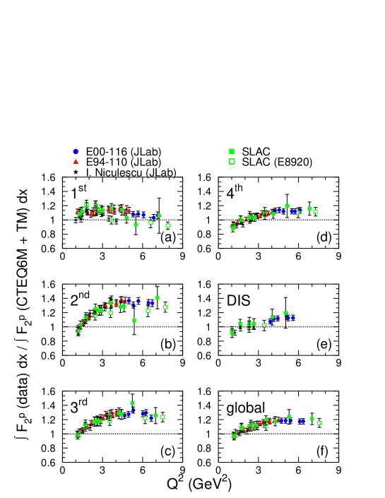
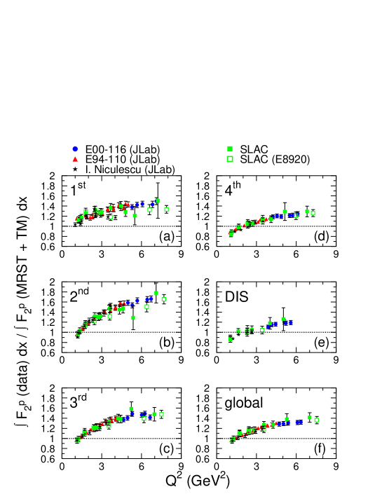
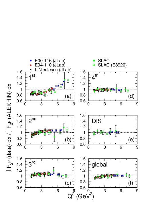
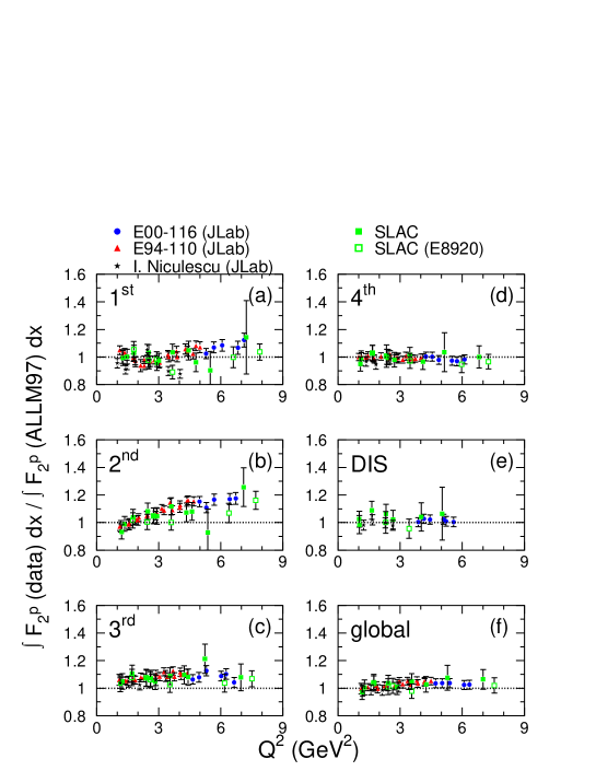
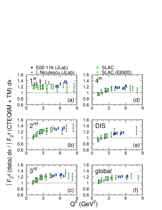
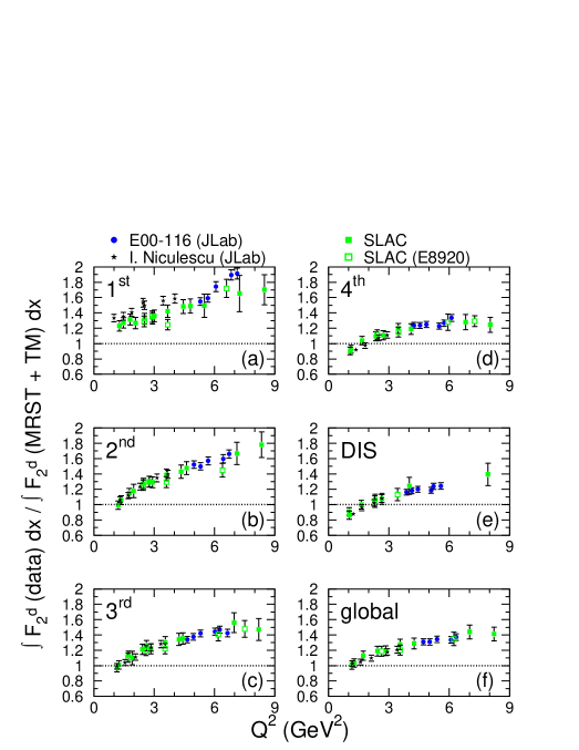
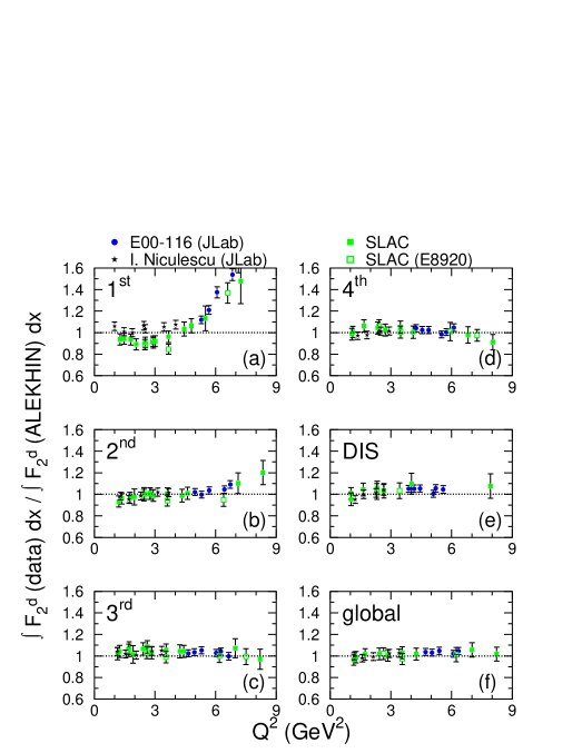
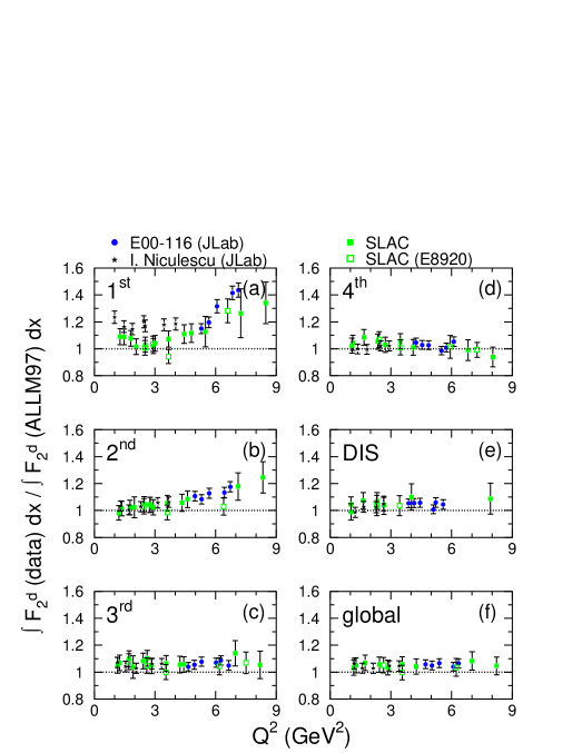
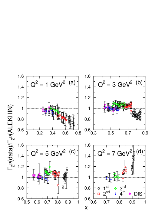
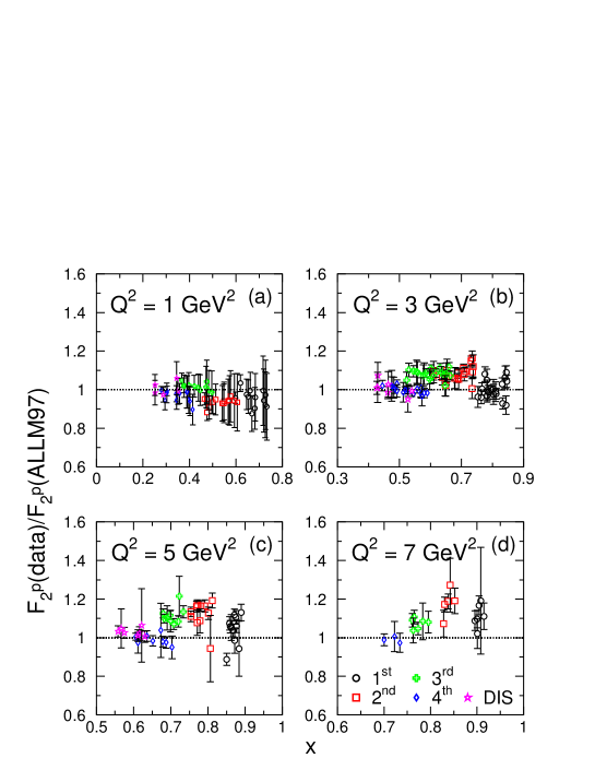
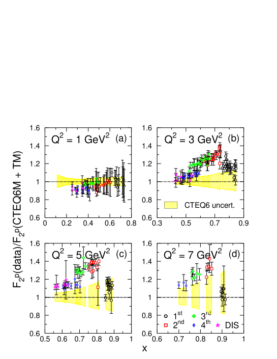
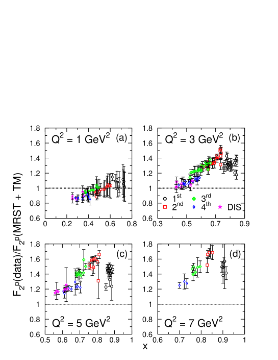
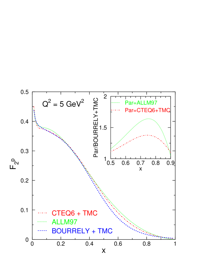
| (H) | stat | syst | (H) | stat | syst | (D) | stat | syst | (D) | stat | syst | |||
|---|---|---|---|---|---|---|---|---|---|---|---|---|---|---|
| 1.5456 | 3.5853 | 4.7162 | 1.3552 | 0.0215 | 0.0208 | 1.3921 | 0.0215 | 0.0156 | 2.1071 | 0.0276 | 0.0319 | 2.1383 | 0.0278 | 0.0242 |
| 1.5623 | 3.6241 | 4.6461 | 1.3206 | 0.0209 | 0.0203 | 1.3507 | 0.0210 | 0.0152 | 2.0745 | 0.0268 | 0.0314 | 2.0941 | 0.0271 | 0.0237 |
| 1.5790 | 3.6629 | 4.5760 | 1.2747 | 0.0200 | 0.0196 | 1.2985 | 0.0202 | 0.0146 | 1.9751 | 0.0255 | 0.0299 | 1.9844 | 0.0259 | 0.0224 |
| 1.5957 | 3.7016 | 4.5059 | 1.2117 | 0.0194 | 0.0186 | 1.2309 | 0.0196 | 0.0138 | 1.9098 | 0.0247 | 0.0289 | 1.9096 | 0.0252 | 0.0216 |
| 1.6124 | 3.7404 | 4.4358 | 1.1546 | 0.0187 | 0.0177 | 1.1680 | 0.0190 | 0.0131 | 1.8305 | 0.0238 | 0.0277 | 1.8221 | 0.0244 | 0.0206 |
| 1.6291 | 3.7791 | 4.3656 | 1.1127 | 0.0182 | 0.0171 | 1.1212 | 0.0185 | 0.0126 | 1.7357 | 0.0229 | 0.0263 | 1.7200 | 0.0236 | 0.0194 |
| 1.6458 | 3.8179 | 4.2955 | 1.1025 | 0.0179 | 0.0169 | 1.1045 | 0.0184 | 0.0124 | 1.6753 | 0.0223 | 0.0254 | 1.6534 | 0.0230 | 0.0187 |
| 1.6625 | 3.8567 | 4.2254 | 1.0683 | 0.0174 | 0.0164 | 1.0668 | 0.0179 | 0.0120 | 1.6388 | 0.0219 | 0.0248 | 1.6102 | 0.0227 | 0.0182 |
| 1.6793 | 3.8954 | 4.1553 | 0.9795 | 0.0165 | 0.0150 | 0.9756 | 0.0170 | 0.0109 | 1.5186 | 0.0207 | 0.0230 | 1.4874 | 0.0216 | 0.0168 |
| 1.6960 | 3.9342 | 4.0852 | 0.9257 | 0.0161 | 0.0142 | 0.9189 | 0.0166 | 0.0103 | 1.4352 | 0.0200 | 0.0218 | 1.4014 | 0.0209 | 0.0158 |
| 1.7127 | 3.9729 | 4.0151 | 0.8999 | 0.0157 | 0.0138 | 0.8897 | 0.0162 | 0.0100 | 1.4014 | 0.0195 | 0.0212 | 1.3632 | 0.0205 | 0.0154 |
| 1.7294 | 4.0117 | 3.9450 | 0.8757 | 0.0153 | 0.0135 | 0.8623 | 0.0160 | 0.0097 | 1.3753 | 0.0193 | 0.0208 | 1.3332 | 0.0203 | 0.0151 |
| 1.7461 | 4.0505 | 3.8748 | 0.8500 | 0.0149 | 0.0131 | 0.8337 | 0.0155 | 0.0094 | 1.2775 | 0.0183 | 0.0194 | 1.2358 | 0.0193 | 0.0140 |
| 1.7628 | 4.0892 | 3.8047 | 0.8408 | 0.0147 | 0.0129 | 0.8209 | 0.0154 | 0.0092 | 1.2525 | 0.0180 | 0.0190 | 1.2076 | 0.0190 | 0.0137 |
| 1.7795 | 4.1280 | 3.7346 | 0.8035 | 0.0142 | 0.0123 | 0.7816 | 0.0149 | 0.0088 | 1.1757 | 0.0172 | 0.0178 | 1.1318 | 0.0182 | 0.0128 |
| 1.7962 | 4.1667 | 3.6645 | 0.7409 | 0.0135 | 0.0114 | 0.7188 | 0.0142 | 0.0081 | 1.1152 | 0.0166 | 0.0169 | 1.0705 | 0.0176 | 0.0121 |
| 1.7973 | 4.1692 | 3.6601 | 0.7589 | 0.0102 | 0.0117 | 0.7352 | 0.0108 | 0.0082 | 1.1433 | 0.0107 | 0.0173 | 1.0962 | 0.0113 | 0.0124 |
| 1.8167 | 4.2143 | 3.5785 | 0.7148 | 0.0097 | 0.0110 | 0.6903 | 0.0102 | 0.0077 | 1.1020 | 0.0102 | 0.0167 | 1.0524 | 0.0109 | 0.0119 |
| 1.8361 | 4.2593 | 3.4970 | 0.6820 | 0.0093 | 0.0105 | 0.6565 | 0.0098 | 0.0074 | 1.0121 | 0.0095 | 0.0153 | 0.9639 | 0.0101 | 0.0109 |
| 1.8556 | 4.3044 | 3.4155 | 0.6232 | 0.0087 | 0.0096 | 0.5993 | 0.0093 | 0.0067 | 0.9622 | 0.0090 | 0.0146 | 0.9125 | 0.0097 | 0.0103 |
| 1.8750 | 4.3495 | 3.3339 | 0.6015 | 0.0085 | 0.0092 | 0.5773 | 0.0091 | 0.0065 | 0.8998 | 0.0087 | 0.0136 | 0.8496 | 0.0093 | 0.0096 |
| 1.8944 | 4.3946 | 3.2524 | 0.5551 | 0.0080 | 0.0085 | 0.5320 | 0.0086 | 0.0060 | 0.8456 | 0.0082 | 0.0128 | 0.7941 | 0.0089 | 0.0090 |
| 1.9139 | 4.4396 | 3.1709 | 0.5318 | 0.0077 | 0.0082 | 0.5070 | 0.0083 | 0.0057 | 0.8058 | 0.0079 | 0.0122 | 0.7520 | 0.0086 | 0.0085 |
| 1.9333 | 4.4847 | 3.0893 | 0.5271 | 0.0077 | 0.0081 | 0.4961 | 0.0083 | 0.0056 | 0.7552 | 0.0075 | 0.0114 | 0.7002 | 0.0082 | 0.0079 |
| 1.9527 | 4.5298 | 3.0078 | 0.5116 | 0.0074 | 0.0079 | 0.4707 | 0.0082 | 0.0053 | 0.7004 | 0.0070 | 0.0106 | 0.6454 | 0.0078 | 0.0073 |
| 1.9721 | 4.5748 | 2.9263 | 0.5150 | 0.0072 | 0.0079 | 0.4637 | 0.0082 | 0.0052 | 0.6366 | 0.0066 | 0.0097 | 0.5837 | 0.0073 | 0.0066 |
| 1.9916 | 4.6199 | 2.8447 | 0.4624 | 0.0066 | 0.0071 | 0.4090 | 0.0076 | 0.0046 | 0.6079 | 0.0063 | 0.0092 | 0.5545 | 0.0071 | 0.0063 |
| 2.0110 | 4.6650 | 2.7632 | 0.4032 | 0.0061 | 0.0062 | 0.3600 | 0.0070 | 0.0040 | 0.5547 | 0.0060 | 0.0084 | 0.5046 | 0.0067 | 0.0057 |
| 2.0304 | 4.7101 | 2.6817 | 0.3493 | 0.0055 | 0.0054 | 0.3173 | 0.0062 | 0.0036 | 0.5063 | 0.0056 | 0.0077 | 0.4597 | 0.0063 | 0.0052 |
| 2.0499 | 4.7551 | 2.6001 | 0.2953 | 0.0050 | 0.0045 | 0.2722 | 0.0056 | 0.0031 | 0.4710 | 0.0053 | 0.0071 | 0.4269 | 0.0060 | 0.0048 |
| 2.0693 | 4.8002 | 2.5186 | 0.2786 | 0.0050 | 0.0043 | 0.2585 | 0.0055 | 0.0029 | 0.4320 | 0.0050 | 0.0066 | 0.3906 | 0.0056 | 0.0044 |
| 2.0887 | 4.8453 | 2.4370 | 0.2701 | 0.0049 | 0.0042 | 0.2491 | 0.0055 | 0.0028 | 0.4007 | 0.0047 | 0.0061 | 0.3610 | 0.0054 | 0.0041 |
| 2.0898 | 4.8477 | 2.4327 | 0.2737 | 0.0035 | 0.0042 | 0.2519 | 0.0039 | 0.0028 | 0.4123 | 0.0036 | 0.0063 | 0.3707 | 0.0041 | 0.0042 |
| 2.1124 | 4.9001 | 2.3379 | 0.2959 | 0.0035 | 0.0046 | 0.2601 | 0.0041 | 0.0029 | 0.3702 | 0.0033 | 0.0056 | 0.3306 | 0.0038 | 0.0037 |
| 2.1349 | 4.9525 | 2.2431 | 0.2671 | 0.0032 | 0.0041 | 0.2266 | 0.0038 | 0.0026 | 0.3394 | 0.0030 | 0.0052 | 0.2998 | 0.0035 | 0.0034 |
| 2.1575 | 5.0049 | 2.1483 | 0.2188 | 0.0027 | 0.0034 | 0.1875 | 0.0033 | 0.0021 | 0.2923 | 0.0027 | 0.0045 | 0.2584 | 0.0032 | 0.0029 |
| 2.1801 | 5.0573 | 2.0535 | 0.1789 | 0.0024 | 0.0028 | 0.1548 | 0.0029 | 0.0018 | 0.2545 | 0.0024 | 0.0039 | 0.2246 | 0.0029 | 0.0026 |
| 2.2027 | 5.1097 | 1.9587 | 0.1442 | 0.0021 | 0.0023 | 0.1252 | 0.0026 | 0.0014 | 0.2271 | 0.0023 | 0.0035 | 0.2002 | 0.0027 | 0.0023 |
| 2.2253 | 5.1621 | 1.8639 | 0.1218 | 0.0019 | 0.0019 | 0.1063 | 0.0023 | 0.0013 | 0.1912 | 0.0020 | 0.0030 | 0.1696 | 0.0024 | 0.0020 |
| 2.2479 | 5.2145 | 1.7691 | 0.0925 | 0.0017 | 0.0015 | 0.0823 | 0.0020 | 0.0010 | 0.1595 | 0.0018 | 0.0026 | 0.1431 | 0.0022 | 0.0017 |
| 2.2705 | 5.2669 | 1.6743 | 0.0816 | 0.0016 | 0.0014 | 0.0727 | 0.0020 | 0.0010 | 0.1342 | 0.0016 | 0.0022 | 0.1227 | 0.0020 | 0.0015 |
| 2.2931 | 5.3193 | 1.5795 | 0.0750 | 0.0016 | 0.0015 | 0.0657 | 0.0020 | 0.0011 | 0.1093 | 0.0015 | 0.0019 | 0.1032 | 0.0018 | 0.0013 |
| 2.3157 | 5.3718 | 1.4847 | 0.0696 | 0.0017 | 0.0017 | 0.0582 | 0.0023 | 0.0013 | 0.0929 | 0.0013 | 0.0018 | 0.0912 | 0.0017 | 0.0012 |
| 2.3383 | 5.4242 | 1.3899 | 0.0405 | 0.0012 | 0.0014 | 0.0354 | 0.0018 | 0.0012 | 0.0796 | 0.0013 | 0.0019 | 0.0816 | 0.0017 | 0.0012 |
| 2.3609 | 5.4766 | 1.2951 | 0.0203 | 0.0009 | 0.0011 | 0.0218 | 0.0014 | 0.0012 | 0.0670 | 0.0011 | 0.0019 | 0.0723 | 0.0015 | 0.0013 |
| 1.4831 | 3.9954 | 4.4235 | 0.8663 | 0.0185 | 0.0133 | 0.8764 | 0.0187 | 0.0098 | 1.2778 | 0.0208 | 0.0194 | 1.2761 | 0.0213 | 0.0144 |
| 1.4991 | 4.0386 | 4.3502 | 0.7946 | 0.0176 | 0.0122 | 0.8019 | 0.0179 | 0.0090 | 1.2380 | 0.0202 | 0.0188 | 1.2305 | 0.0208 | 0.0139 |
| 1.5151 | 4.0818 | 4.2769 | 0.7645 | 0.0167 | 0.0117 | 0.7684 | 0.0170 | 0.0086 | 1.1795 | 0.0193 | 0.0179 | 1.1689 | 0.0199 | 0.0132 |
| 1.5312 | 4.1250 | 4.2036 | 0.7400 | 0.0164 | 0.0114 | 0.7408 | 0.0168 | 0.0083 | 1.1221 | 0.0186 | 0.0170 | 1.1068 | 0.0192 | 0.0125 |
| 1.5472 | 4.1682 | 4.1303 | 0.7246 | 0.0161 | 0.0111 | 0.7221 | 0.0166 | 0.0081 | 1.0686 | 0.0179 | 0.0162 | 1.0499 | 0.0187 | 0.0119 |
| 1.5632 | 4.2114 | 4.0571 | 0.6731 | 0.0152 | 0.0103 | 0.6686 | 0.0157 | 0.0075 | 1.0422 | 0.0174 | 0.0158 | 1.0200 | 0.0182 | 0.0115 |
| 1.5793 | 4.2546 | 3.9838 | 0.6490 | 0.0149 | 0.0100 | 0.6418 | 0.0155 | 0.0072 | 0.9415 | 0.0164 | 0.0143 | 0.9193 | 0.0172 | 0.0104 |
| 1.5953 | 4.2978 | 3.9105 | 0.6325 | 0.0147 | 0.0097 | 0.6228 | 0.0153 | 0.0070 | 0.9152 | 0.0161 | 0.0139 | 0.8904 | 0.0169 | 0.0101 |
| 1.6113 | 4.3410 | 3.8372 | 0.6119 | 0.0143 | 0.0094 | 0.5998 | 0.0150 | 0.0067 | 0.8736 | 0.0155 | 0.0132 | 0.8473 | 0.0163 | 0.0096 |
| 1.6273 | 4.3842 | 3.7639 | 0.5512 | 0.0135 | 0.0085 | 0.5390 | 0.0142 | 0.0060 | 0.8480 | 0.0152 | 0.0129 | 0.8196 | 0.0161 | 0.0093 |
| 1.6434 | 4.4274 | 3.6907 | 0.5340 | 0.0132 | 0.0082 | 0.5199 | 0.0139 | 0.0058 | 0.7789 | 0.0145 | 0.0118 | 0.7510 | 0.0154 | 0.0085 |
| 1.6594 | 4.4706 | 3.6174 | 0.5193 | 0.0131 | 0.0080 | 0.5035 | 0.0138 | 0.0056 | 0.7367 | 0.0141 | 0.0112 | 0.7082 | 0.0149 | 0.0080 |
| 1.6754 | 4.5138 | 3.5441 | 0.4758 | 0.0124 | 0.0073 | 0.4603 | 0.0132 | 0.0052 | 0.7148 | 0.0138 | 0.0108 | 0.6846 | 0.0147 | 0.0077 |
| 1.6915 | 4.5570 | 3.4708 | 0.4524 | 0.0120 | 0.0070 | 0.4367 | 0.0128 | 0.0049 | 0.6694 | 0.0133 | 0.0102 | 0.6393 | 0.0142 | 0.0072 |
| (H) | stat | syst | (H) | stat | syst | (D) | stat | syst | (D) | stat | syst | |||
|---|---|---|---|---|---|---|---|---|---|---|---|---|---|---|
| 1.7075 | 4.6001 | 3.3975 | 0.4201 | 0.0116 | 0.0065 | 0.4054 | 0.0123 | 0.0045 | 0.6431 | 0.0128 | 0.0098 | 0.6117 | 0.0137 | 0.0069 |
| 1.7235 | 4.6433 | 3.3243 | 0.4230 | 0.0113 | 0.0065 | 0.4071 | 0.0120 | 0.0046 | 0.5836 | 0.0120 | 0.0089 | 0.5534 | 0.0129 | 0.0063 |
| 1.7244 | 4.6456 | 3.3204 | 0.4093 | 0.0064 | 0.0063 | 0.3939 | 0.0068 | 0.0044 | 0.5993 | 0.0068 | 0.0091 | 0.5674 | 0.0073 | 0.0064 |
| 1.7430 | 4.6958 | 3.2352 | 0.3807 | 0.0060 | 0.0058 | 0.3659 | 0.0064 | 0.0041 | 0.5712 | 0.0065 | 0.0087 | 0.5377 | 0.0071 | 0.0061 |
| 1.7617 | 4.7460 | 3.1500 | 0.3693 | 0.0058 | 0.0057 | 0.3528 | 0.0062 | 0.0040 | 0.5378 | 0.0061 | 0.0082 | 0.5031 | 0.0066 | 0.0057 |
| 1.7803 | 4.7963 | 3.0648 | 0.3606 | 0.0057 | 0.0055 | 0.3394 | 0.0062 | 0.0038 | 0.5111 | 0.0059 | 0.0078 | 0.4748 | 0.0065 | 0.0054 |
| 1.7990 | 4.8465 | 2.9796 | 0.3687 | 0.0056 | 0.0057 | 0.3379 | 0.0062 | 0.0038 | 0.4707 | 0.0055 | 0.0071 | 0.4345 | 0.0061 | 0.0049 |
| 1.8176 | 4.8967 | 2.8944 | 0.3350 | 0.0052 | 0.0051 | 0.3003 | 0.0059 | 0.0034 | 0.4412 | 0.0052 | 0.0067 | 0.4048 | 0.0058 | 0.0046 |
| 1.8362 | 4.9469 | 2.8092 | 0.3029 | 0.0047 | 0.0047 | 0.2682 | 0.0055 | 0.0030 | 0.3902 | 0.0048 | 0.0059 | 0.3568 | 0.0054 | 0.0040 |
| 1.8549 | 4.9972 | 2.7240 | 0.2416 | 0.0042 | 0.0037 | 0.2176 | 0.0047 | 0.0024 | 0.3643 | 0.0046 | 0.0055 | 0.3320 | 0.0052 | 0.0038 |
| 1.8735 | 5.0474 | 2.6388 | 0.2065 | 0.0038 | 0.0032 | 0.1900 | 0.0042 | 0.0021 | 0.3191 | 0.0042 | 0.0048 | 0.2906 | 0.0048 | 0.0033 |
| 1.8922 | 5.0976 | 2.5536 | 0.1809 | 0.0035 | 0.0028 | 0.1687 | 0.0039 | 0.0019 | 0.2912 | 0.0040 | 0.0044 | 0.2646 | 0.0045 | 0.0030 |
| 1.9108 | 5.1478 | 2.4684 | 0.1664 | 0.0035 | 0.0026 | 0.1556 | 0.0039 | 0.0017 | 0.2737 | 0.0038 | 0.0042 | 0.2479 | 0.0044 | 0.0028 |
| 1.9294 | 5.1980 | 2.3832 | 0.1810 | 0.0037 | 0.0028 | 0.1656 | 0.0042 | 0.0019 | 0.2485 | 0.0036 | 0.0038 | 0.2239 | 0.0041 | 0.0025 |
| 1.9481 | 5.2483 | 2.2980 | 0.1802 | 0.0036 | 0.0028 | 0.1562 | 0.0043 | 0.0018 | 0.2217 | 0.0034 | 0.0034 | 0.1983 | 0.0039 | 0.0022 |
| 1.9667 | 5.2985 | 2.2128 | 0.1649 | 0.0033 | 0.0025 | 0.1395 | 0.0040 | 0.0016 | 0.2068 | 0.0032 | 0.0032 | 0.1828 | 0.0037 | 0.0021 |
| 1.9854 | 5.3487 | 2.1276 | 0.1410 | 0.0028 | 0.0022 | 0.1206 | 0.0035 | 0.0014 | 0.1870 | 0.0029 | 0.0029 | 0.1654 | 0.0034 | 0.0019 |
| 2.0040 | 5.3989 | 2.0424 | 0.1089 | 0.0024 | 0.0017 | 0.0947 | 0.0029 | 0.0011 | 0.1648 | 0.0027 | 0.0025 | 0.1464 | 0.0032 | 0.0017 |
| 2.0051 | 5.4019 | 2.0373 | 0.1060 | 0.0014 | 0.0016 | 0.0923 | 0.0017 | 0.0011 | 0.1679 | 0.0019 | 0.0026 | 0.1488 | 0.0022 | 0.0017 |
| 2.0268 | 5.4603 | 1.9382 | 0.0885 | 0.0013 | 0.0014 | 0.0774 | 0.0015 | 0.0009 | 0.1345 | 0.0016 | 0.0021 | 0.1201 | 0.0020 | 0.0014 |
| 2.0485 | 5.5187 | 1.8391 | 0.0718 | 0.0011 | 0.0011 | 0.0632 | 0.0014 | 0.0008 | 0.1214 | 0.0015 | 0.0019 | 0.1086 | 0.0018 | 0.0012 |
| 2.0702 | 5.5771 | 1.7401 | 0.0560 | 0.0010 | 0.0009 | 0.0503 | 0.0012 | 0.0006 | 0.0981 | 0.0013 | 0.0016 | 0.0892 | 0.0016 | 0.0010 |
| 2.0918 | 5.6355 | 1.6410 | 0.0520 | 0.0010 | 0.0009 | 0.0465 | 0.0012 | 0.0007 | 0.0830 | 0.0012 | 0.0014 | 0.0772 | 0.0015 | 0.0009 |
| 2.1135 | 5.6939 | 1.5419 | 0.0503 | 0.0010 | 0.0011 | 0.0438 | 0.0012 | 0.0008 | 0.0625 | 0.0010 | 0.0011 | 0.0611 | 0.0013 | 0.0008 |
| 2.1352 | 5.7523 | 1.4428 | 0.0407 | 0.0010 | 0.0012 | 0.0338 | 0.0014 | 0.0009 | 0.0547 | 0.0010 | 0.0012 | 0.0556 | 0.0013 | 0.0008 |
| 2.1569 | 5.8107 | 1.3437 | 0.0182 | 0.0006 | 0.0008 | 0.0173 | 0.0009 | 0.0007 | 0.0487 | 0.0009 | 0.0013 | 0.0510 | 0.0012 | 0.0009 |
| 2.1785 | 5.8691 | 1.2447 | 0.0062 | 0.0004 | 0.0004 | 0.0129 | 0.0007 | 0.0009 | 0.0389 | 0.0008 | 0.0014 | 0.0435 | 0.0011 | 0.0010 |
| 1.3308 | 4.2817 | 4.4229 | 0.5780 | 0.0128 | 0.0089 | 0.5884 | 0.0130 | 0.0066 | 0.8757 | 0.0147 | 0.0133 | 0.8806 | 0.0150 | 0.0100 |
| 1.3452 | 4.3280 | 4.3496 | 0.5583 | 0.0123 | 0.0086 | 0.5660 | 0.0125 | 0.0063 | 0.8315 | 0.0141 | 0.0126 | 0.8329 | 0.0145 | 0.0094 |
| 1.3596 | 4.3743 | 4.2763 | 0.5494 | 0.0118 | 0.0084 | 0.5543 | 0.0121 | 0.0062 | 0.7993 | 0.0135 | 0.0121 | 0.7973 | 0.0139 | 0.0090 |
| 1.3740 | 4.4206 | 4.2031 | 0.4809 | 0.0111 | 0.0074 | 0.4847 | 0.0113 | 0.0054 | 0.7488 | 0.0130 | 0.0114 | 0.7443 | 0.0134 | 0.0084 |
| 1.3883 | 4.4668 | 4.1298 | 0.4764 | 0.0109 | 0.0073 | 0.4777 | 0.0112 | 0.0054 | 0.7165 | 0.0125 | 0.0109 | 0.7094 | 0.0129 | 0.0080 |
| 1.4027 | 4.5131 | 4.0565 | 0.4544 | 0.0105 | 0.0070 | 0.4537 | 0.0108 | 0.0051 | 0.6773 | 0.0121 | 0.0103 | 0.6682 | 0.0126 | 0.0076 |
| 1.4171 | 4.5594 | 3.9832 | 0.4213 | 0.0100 | 0.0065 | 0.4192 | 0.0104 | 0.0047 | 0.6539 | 0.0118 | 0.0099 | 0.6426 | 0.0123 | 0.0073 |
| 1.4315 | 4.6057 | 3.9099 | 0.3955 | 0.0098 | 0.0061 | 0.3922 | 0.0101 | 0.0044 | 0.6223 | 0.0114 | 0.0094 | 0.6096 | 0.0119 | 0.0069 |
| 1.4459 | 4.6520 | 3.8366 | 0.3889 | 0.0096 | 0.0060 | 0.3838 | 0.0100 | 0.0043 | 0.5932 | 0.0110 | 0.0090 | 0.5790 | 0.0115 | 0.0066 |
| 1.4603 | 4.6983 | 3.7633 | 0.3559 | 0.0090 | 0.0055 | 0.3502 | 0.0094 | 0.0039 | 0.5211 | 0.0102 | 0.0079 | 0.5080 | 0.0107 | 0.0057 |
| 1.4747 | 4.7446 | 3.6901 | 0.3590 | 0.0090 | 0.0055 | 0.3513 | 0.0095 | 0.0039 | 0.5106 | 0.0101 | 0.0077 | 0.4957 | 0.0106 | 0.0056 |
| 1.4891 | 4.7909 | 3.6168 | 0.3255 | 0.0086 | 0.0050 | 0.3178 | 0.0090 | 0.0036 | 0.5001 | 0.0100 | 0.0076 | 0.4837 | 0.0105 | 0.0055 |
| 1.5034 | 4.8372 | 3.5435 | 0.2999 | 0.0082 | 0.0046 | 0.2923 | 0.0086 | 0.0033 | 0.4644 | 0.0095 | 0.0070 | 0.4478 | 0.0101 | 0.0051 |
| 1.5178 | 4.8834 | 3.4702 | 0.2983 | 0.0081 | 0.0046 | 0.2896 | 0.0085 | 0.0032 | 0.4466 | 0.0092 | 0.0068 | 0.4290 | 0.0098 | 0.0049 |
| 1.5322 | 4.9297 | 3.3969 | 0.2710 | 0.0076 | 0.0042 | 0.2632 | 0.0081 | 0.0030 | 0.4049 | 0.0086 | 0.0061 | 0.3879 | 0.0092 | 0.0044 |
| 1.5466 | 4.9760 | 3.3236 | 0.2653 | 0.0074 | 0.0041 | 0.2571 | 0.0079 | 0.0029 | 0.3978 | 0.0084 | 0.0060 | 0.3791 | 0.0090 | 0.0043 |
| 1.5474 | 4.9787 | 3.3194 | 0.2636 | 0.0049 | 0.0041 | 0.2553 | 0.0052 | 0.0029 | 0.4027 | 0.0052 | 0.0061 | 0.3833 | 0.0056 | 0.0043 |
| 1.5642 | 5.0325 | 3.2342 | 0.2402 | 0.0046 | 0.0037 | 0.2325 | 0.0050 | 0.0026 | 0.3733 | 0.0049 | 0.0057 | 0.3535 | 0.0053 | 0.0040 |
| 1.5809 | 5.0863 | 3.1490 | 0.2311 | 0.0045 | 0.0036 | 0.2224 | 0.0048 | 0.0025 | 0.3494 | 0.0047 | 0.0053 | 0.3288 | 0.0051 | 0.0037 |
| 1.5976 | 5.1402 | 3.0637 | 0.2419 | 0.0045 | 0.0037 | 0.2288 | 0.0049 | 0.0026 | 0.3297 | 0.0044 | 0.0050 | 0.3081 | 0.0048 | 0.0035 |
| 1.6143 | 5.1940 | 2.9785 | 0.2407 | 0.0044 | 0.0037 | 0.2219 | 0.0049 | 0.0025 | 0.3108 | 0.0042 | 0.0047 | 0.2883 | 0.0047 | 0.0033 |
| 1.6311 | 5.2478 | 2.8933 | 0.2297 | 0.0042 | 0.0035 | 0.2067 | 0.0047 | 0.0023 | 0.2786 | 0.0039 | 0.0042 | 0.2573 | 0.0044 | 0.0029 |
| 1.6478 | 5.3016 | 2.8081 | 0.1955 | 0.0037 | 0.0030 | 0.1742 | 0.0043 | 0.0020 | 0.2588 | 0.0038 | 0.0039 | 0.2379 | 0.0042 | 0.0027 |
| 1.6645 | 5.3555 | 2.7229 | 0.1634 | 0.0034 | 0.0025 | 0.1480 | 0.0038 | 0.0017 | 0.2356 | 0.0035 | 0.0036 | 0.2160 | 0.0039 | 0.0024 |
| 1.6813 | 5.4093 | 2.6377 | 0.1392 | 0.0031 | 0.0021 | 0.1288 | 0.0035 | 0.0014 | 0.2098 | 0.0033 | 0.0032 | 0.1920 | 0.0037 | 0.0022 |
| 1.6980 | 5.4631 | 2.5525 | 0.1200 | 0.0029 | 0.0018 | 0.1124 | 0.0032 | 0.0013 | 0.1855 | 0.0030 | 0.0028 | 0.1696 | 0.0034 | 0.0019 |
| 1.7147 | 5.5169 | 2.4672 | 0.1038 | 0.0028 | 0.0016 | 0.0978 | 0.0030 | 0.0011 | 0.1656 | 0.0028 | 0.0025 | 0.1510 | 0.0032 | 0.0017 |
| 1.7315 | 5.5707 | 2.3820 | 0.1088 | 0.0029 | 0.0017 | 0.1002 | 0.0032 | 0.0011 | 0.1615 | 0.0028 | 0.0025 | 0.1460 | 0.0032 | 0.0017 |
| 1.7482 | 5.6246 | 2.2968 | 0.1343 | 0.0031 | 0.0021 | 0.1165 | 0.0038 | 0.0013 | 0.1506 | 0.0026 | 0.0023 | 0.1350 | 0.0031 | 0.0015 |
| 1.7649 | 5.6784 | 2.2116 | 0.1111 | 0.0027 | 0.0017 | 0.0946 | 0.0032 | 0.0011 | 0.1320 | 0.0024 | 0.0020 | 0.1175 | 0.0028 | 0.0013 |
| 1.7816 | 5.7322 | 2.1264 | 0.0846 | 0.0022 | 0.0013 | 0.0728 | 0.0026 | 0.0008 | 0.1194 | 0.0022 | 0.0018 | 0.1066 | 0.0026 | 0.0012 |
| 1.7984 | 5.7860 | 2.0412 | 0.0708 | 0.0020 | 0.0011 | 0.0618 | 0.0024 | 0.0007 | 0.0999 | 0.0020 | 0.0015 | 0.0896 | 0.0024 | 0.0010 |
| (H) | stat | syst | (H) | stat | syst | (D) | stat | syst | (D) | stat | syst | |||
|---|---|---|---|---|---|---|---|---|---|---|---|---|---|---|
| 1.7994 | 5.7894 | 2.0359 | 0.0658 | 0.0010 | 0.0010 | 0.0576 | 0.0012 | 0.0007 | 0.1043 | 0.0024 | 0.0016 | 0.0932 | 0.0028 | 0.0011 |
| 1.8189 | 5.8520 | 1.9368 | 0.0568 | 0.0009 | 0.0009 | 0.0498 | 0.0010 | 0.0006 | 0.0929 | 0.0023 | 0.0014 | 0.0830 | 0.0027 | 0.0010 |
| 1.8383 | 5.9145 | 1.8377 | 0.0456 | 0.0008 | 0.0007 | 0.0403 | 0.0009 | 0.0005 | 0.0752 | 0.0019 | 0.0012 | 0.0679 | 0.0023 | 0.0008 |
| 1.8578 | 5.9771 | 1.7386 | 0.0346 | 0.0007 | 0.0006 | 0.0312 | 0.0008 | 0.0004 | 0.0594 | 0.0017 | 0.0010 | 0.0546 | 0.0021 | 0.0006 |
| 1.8772 | 6.0397 | 1.6395 | 0.0307 | 0.0007 | 0.0006 | 0.0277 | 0.0008 | 0.0004 | 0.0524 | 0.0016 | 0.0009 | 0.0491 | 0.0019 | 0.0006 |
| 1.8967 | 6.1023 | 1.5404 | 0.0294 | 0.0007 | 0.0006 | 0.0258 | 0.0008 | 0.0005 | 0.0424 | 0.0014 | 0.0008 | 0.0411 | 0.0018 | 0.0005 |
| 1.9161 | 6.1649 | 1.4413 | 0.0238 | 0.0007 | 0.0007 | 0.0200 | 0.0010 | 0.0005 | 0.0404 | 0.0014 | 0.0008 | 0.0398 | 0.0018 | 0.0005 |
| 1.9356 | 6.2275 | 1.3422 | 0.0118 | 0.0005 | 0.0005 | 0.0112 | 0.0008 | 0.0005 | 0.0351 | 0.0014 | 0.0009 | 0.0353 | 0.0018 | 0.0005 |
| 1.9550 | 6.2901 | 1.2431 | 0.0083 | 0.0005 | 0.0006 | 0.0115 | 0.0007 | 0.0008 | 0.0258 | 0.0010 | 0.0008 | 0.0278 | 0.0015 | 0.0005 |
| 1.0699 | 5.0150 | 4.1791 | 0.2387 | 0.0054 | 0.0037 | 0.2444 | 0.0055 | 0.0027 | 0.3316 | 0.0049 | 0.0050 | 0.3379 | 0.0050 | 0.0038 |
| 1.0815 | 5.0692 | 4.1032 | 0.2160 | 0.0051 | 0.0033 | 0.2208 | 0.0052 | 0.0025 | 0.3061 | 0.0047 | 0.0046 | 0.3110 | 0.0048 | 0.0035 |
| 1.0931 | 5.1234 | 4.0273 | 0.2025 | 0.0050 | 0.0031 | 0.2064 | 0.0051 | 0.0023 | 0.2916 | 0.0045 | 0.0044 | 0.2951 | 0.0046 | 0.0033 |
| 1.1046 | 5.1776 | 3.9513 | 0.1942 | 0.0047 | 0.0030 | 0.1969 | 0.0048 | 0.0022 | 0.2775 | 0.0043 | 0.0042 | 0.2797 | 0.0044 | 0.0032 |
| 1.1162 | 5.2319 | 3.8754 | 0.1818 | 0.0046 | 0.0028 | 0.1838 | 0.0047 | 0.0021 | 0.2624 | 0.0042 | 0.0040 | 0.2635 | 0.0043 | 0.0030 |
| 1.1278 | 5.2861 | 3.7995 | 0.1659 | 0.0043 | 0.0025 | 0.1672 | 0.0044 | 0.0019 | 0.2342 | 0.0039 | 0.0036 | 0.2346 | 0.0040 | 0.0027 |
| 1.1393 | 5.3403 | 3.7236 | 0.1609 | 0.0042 | 0.0025 | 0.1613 | 0.0043 | 0.0018 | 0.2236 | 0.0038 | 0.0034 | 0.2233 | 0.0040 | 0.0025 |
| 1.1509 | 5.3945 | 3.6477 | 0.1551 | 0.0040 | 0.0024 | 0.1548 | 0.0041 | 0.0017 | 0.2171 | 0.0037 | 0.0033 | 0.2154 | 0.0038 | 0.0024 |
| 1.1625 | 5.4487 | 3.5717 | 0.1325 | 0.0038 | 0.0020 | 0.1322 | 0.0039 | 0.0015 | 0.2020 | 0.0035 | 0.0031 | 0.1998 | 0.0037 | 0.0023 |
| 1.1741 | 5.5029 | 3.4958 | 0.1260 | 0.0036 | 0.0019 | 0.1254 | 0.0038 | 0.0014 | 0.1900 | 0.0034 | 0.0029 | 0.1871 | 0.0036 | 0.0021 |
| 1.1856 | 5.5572 | 3.4199 | 0.1209 | 0.0035 | 0.0019 | 0.1201 | 0.0037 | 0.0013 | 0.1756 | 0.0032 | 0.0027 | 0.1722 | 0.0034 | 0.0020 |
| 1.1972 | 5.6114 | 3.3440 | 0.1139 | 0.0035 | 0.0017 | 0.1129 | 0.0036 | 0.0013 | 0.1661 | 0.0031 | 0.0025 | 0.1623 | 0.0033 | 0.0018 |
| 1.2088 | 5.6656 | 3.2680 | 0.1060 | 0.0033 | 0.0016 | 0.1050 | 0.0034 | 0.0012 | 0.1559 | 0.0030 | 0.0024 | 0.1512 | 0.0032 | 0.0017 |
| 1.2203 | 5.7198 | 3.1921 | 0.1036 | 0.0032 | 0.0016 | 0.1022 | 0.0034 | 0.0011 | 0.1459 | 0.0029 | 0.0022 | 0.1411 | 0.0031 | 0.0016 |
| 1.2319 | 5.7740 | 3.1162 | 0.0962 | 0.0030 | 0.0015 | 0.0943 | 0.0032 | 0.0011 | 0.1421 | 0.0028 | 0.0022 | 0.1362 | 0.0030 | 0.0015 |
| 1.2435 | 5.8282 | 3.0403 | 0.0987 | 0.0029 | 0.0015 | 0.0950 | 0.0032 | 0.0011 | 0.1313 | 0.0026 | 0.0020 | 0.1252 | 0.0028 | 0.0014 |
| 1.2442 | 5.8318 | 3.0353 | 0.0994 | 0.0014 | 0.0015 | 0.0955 | 0.0015 | 0.0011 | 0.1373 | 0.0015 | 0.0021 | 0.1305 | 0.0016 | 0.0015 |
| 1.2577 | 5.8949 | 2.9470 | 0.0972 | 0.0014 | 0.0015 | 0.0908 | 0.0015 | 0.0010 | 0.1232 | 0.0013 | 0.0019 | 0.1165 | 0.0015 | 0.0013 |
| 1.2711 | 5.9579 | 2.8587 | 0.0907 | 0.0013 | 0.0014 | 0.0826 | 0.0015 | 0.0009 | 0.1116 | 0.0013 | 0.0017 | 0.1050 | 0.0014 | 0.0012 |
| 1.2846 | 6.0210 | 2.7704 | 0.0765 | 0.0011 | 0.0012 | 0.0697 | 0.0013 | 0.0008 | 0.1037 | 0.0012 | 0.0016 | 0.0971 | 0.0013 | 0.0011 |
| 1.2980 | 6.0840 | 2.6821 | 0.0598 | 0.0010 | 0.0009 | 0.0561 | 0.0011 | 0.0006 | 0.0918 | 0.0011 | 0.0014 | 0.0858 | 0.0012 | 0.0010 |
| 1.3115 | 6.1471 | 2.5938 | 0.0488 | 0.0009 | 0.0008 | 0.0468 | 0.0010 | 0.0005 | 0.0816 | 0.0010 | 0.0012 | 0.0761 | 0.0012 | 0.0009 |
| 1.3249 | 6.2101 | 2.5055 | 0.0456 | 0.0009 | 0.0007 | 0.0440 | 0.0010 | 0.0005 | 0.0737 | 0.0010 | 0.0011 | 0.0685 | 0.0011 | 0.0008 |
| 1.3384 | 6.2732 | 2.4172 | 0.0435 | 0.0009 | 0.0007 | 0.0417 | 0.0010 | 0.0005 | 0.0632 | 0.0009 | 0.0010 | 0.0587 | 0.0010 | 0.0007 |
| 1.3518 | 6.3362 | 2.3290 | 0.0472 | 0.0009 | 0.0007 | 0.0428 | 0.0011 | 0.0005 | 0.0587 | 0.0009 | 0.0009 | 0.0541 | 0.0010 | 0.0006 |
| 1.3653 | 6.3992 | 2.2407 | 0.0458 | 0.0009 | 0.0007 | 0.0399 | 0.0011 | 0.0004 | 0.0547 | 0.0008 | 0.0008 | 0.0499 | 0.0009 | 0.0006 |
| 1.3787 | 6.4623 | 2.1524 | 0.0355 | 0.0008 | 0.0005 | 0.0308 | 0.0009 | 0.0003 | 0.0481 | 0.0008 | 0.0007 | 0.0437 | 0.0009 | 0.0005 |
| 1.3922 | 6.5253 | 2.0641 | 0.0281 | 0.0006 | 0.0004 | 0.0249 | 0.0008 | 0.0003 | 0.0418 | 0.0007 | 0.0006 | 0.0384 | 0.0008 | 0.0004 |
| 1.4056 | 6.5884 | 1.9758 | 0.0231 | 0.0006 | 0.0004 | 0.0207 | 0.0007 | 0.0002 | 0.0381 | 0.0007 | 0.0006 | 0.0348 | 0.0007 | 0.0004 |
| 1.4191 | 6.6514 | 1.8875 | 0.0195 | 0.0005 | 0.0003 | 0.0174 | 0.0006 | 0.0002 | 0.0314 | 0.0006 | 0.0005 | 0.0290 | 0.0007 | 0.0003 |
| 1.4325 | 6.7145 | 1.7992 | 0.0147 | 0.0005 | 0.0002 | 0.0133 | 0.0006 | 0.0002 | 0.0272 | 0.0006 | 0.0004 | 0.0253 | 0.0007 | 0.0003 |
| 1.4460 | 6.7775 | 1.7109 | 0.0137 | 0.0005 | 0.0002 | 0.0124 | 0.0006 | 0.0001 | 0.0233 | 0.0005 | 0.0004 | 0.0220 | 0.0006 | 0.0003 |
| 1.3622 | 6.3850 | 2.2605 | 0.0458 | 0.0010 | 0.0007 | 0.0399 | 0.0012 | 0.0005 | 0.0592 | 0.0009 | 0.0009 | 0.0540 | 0.0010 | 0.0006 |
| 1.3770 | 6.4541 | 2.1639 | 0.0368 | 0.0008 | 0.0006 | 0.0316 | 0.0010 | 0.0004 | 0.0517 | 0.0008 | 0.0008 | 0.0469 | 0.0009 | 0.0005 |
| 1.3917 | 6.5231 | 2.0672 | 0.0282 | 0.0007 | 0.0004 | 0.0249 | 0.0008 | 0.0003 | 0.0429 | 0.0007 | 0.0007 | 0.0392 | 0.0009 | 0.0005 |
| 1.4064 | 6.5921 | 1.9706 | 0.0235 | 0.0007 | 0.0004 | 0.0209 | 0.0008 | 0.0003 | 0.0380 | 0.0007 | 0.0006 | 0.0348 | 0.0008 | 0.0004 |
| 1.4212 | 6.6612 | 1.8739 | 0.0187 | 0.0006 | 0.0003 | 0.0165 | 0.0007 | 0.0002 | 0.0326 | 0.0006 | 0.0005 | 0.0300 | 0.0007 | 0.0004 |
| 1.4359 | 6.7302 | 1.7772 | 0.0139 | 0.0005 | 0.0002 | 0.0125 | 0.0006 | 0.0002 | 0.0271 | 0.0006 | 0.0004 | 0.0252 | 0.0007 | 0.0003 |
| 1.4506 | 6.7992 | 1.6806 | 0.0119 | 0.0005 | 0.0002 | 0.0109 | 0.0006 | 0.0001 | 0.0234 | 0.0005 | 0.0004 | 0.0222 | 0.0006 | 0.0003 |
| 1.4653 | 6.8682 | 1.5839 | 0.0110 | 0.0005 | 0.0002 | 0.0099 | 0.0006 | 0.0002 | 0.0199 | 0.0005 | 0.0003 | 0.0192 | 0.0006 | 0.0002 |
| 1.4801 | 6.9373 | 1.4872 | 0.0094 | 0.0005 | 0.0002 | 0.0082 | 0.0006 | 0.0002 | 0.0169 | 0.0005 | 0.0003 | 0.0167 | 0.0006 | 0.0002 |
| 1.4948 | 7.0063 | 1.3906 | 0.0070 | 0.0003 | 0.0002 | 0.0059 | 0.0005 | 0.0002 | 0.0168 | 0.0005 | 0.0004 | 0.0165 | 0.0006 | 0.0002 |
| 1.5095 | 7.0753 | 1.2939 | 0.0034 | 0.0002 | 0.0002 | 0.0034 | 0.0003 | 0.0002 | 0.0137 | 0.0004 | 0.0004 | 0.0137 | 0.0006 | 0.0002 |
| 0.8234 | 4.5252 | 5.1315 | 0.3212 | 0.0115 | 0.0049 | 0.3569 | 0.0111 | 0.0040 | 0.5071 | 0.0130 | 0.0077 | 0.5602 | 0.0125 | 0.0064 |
| 0.8323 | 4.5741 | 5.0659 | 0.3289 | 0.0115 | 0.0051 | 0.3623 | 0.0111 | 0.0041 | 0.4487 | 0.0122 | 0.0068 | 0.4966 | 0.0118 | 0.0056 |
| 0.8412 | 4.6230 | 5.0003 | 0.3035 | 0.0107 | 0.0047 | 0.3335 | 0.0104 | 0.0037 | 0.4580 | 0.0120 | 0.0070 | 0.5030 | 0.0116 | 0.0057 |
| 0.8501 | 4.6719 | 4.9347 | 0.2749 | 0.0100 | 0.0042 | 0.3017 | 0.0097 | 0.0034 | 0.4263 | 0.0114 | 0.0065 | 0.4668 | 0.0111 | 0.0053 |
| 0.8590 | 4.7209 | 4.8690 | 0.2692 | 0.0098 | 0.0041 | 0.2934 | 0.0096 | 0.0033 | 0.3912 | 0.0108 | 0.0060 | 0.4270 | 0.0105 | 0.0049 |
| 0.8679 | 4.7698 | 4.8034 | 0.2640 | 0.0097 | 0.0041 | 0.2859 | 0.0095 | 0.0032 | 0.3956 | 0.0106 | 0.0060 | 0.4278 | 0.0104 | 0.0049 |
| 0.8768 | 4.8187 | 4.7378 | 0.2396 | 0.0092 | 0.0037 | 0.2589 | 0.0091 | 0.0029 | 0.3781 | 0.0105 | 0.0058 | 0.4065 | 0.0103 | 0.0046 |
| (H) | stat | syst | (H) | stat | syst | (D) | stat | syst | (D) | stat | syst | |||
|---|---|---|---|---|---|---|---|---|---|---|---|---|---|---|
| 0.8857 | 4.8676 | 4.6722 | 0.2333 | 0.0090 | 0.0036 | 0.2507 | 0.0089 | 0.0028 | 0.3579 | 0.0099 | 0.0054 | 0.3828 | 0.0098 | 0.0044 |
| 0.8947 | 4.9165 | 4.6065 | 0.2130 | 0.0085 | 0.0033 | 0.2283 | 0.0085 | 0.0026 | 0.3515 | 0.0096 | 0.0053 | 0.3736 | 0.0095 | 0.0043 |
| 0.9036 | 4.9655 | 4.5409 | 0.2124 | 0.0084 | 0.0033 | 0.2261 | 0.0084 | 0.0025 | 0.3200 | 0.0093 | 0.0049 | 0.3392 | 0.0093 | 0.0039 |
| 0.9125 | 5.0144 | 4.4753 | 0.1982 | 0.0081 | 0.0030 | 0.2104 | 0.0081 | 0.0024 | 0.2887 | 0.0087 | 0.0044 | 0.3055 | 0.0086 | 0.0035 |
| 0.9214 | 5.0633 | 4.4096 | 0.1970 | 0.0079 | 0.0030 | 0.2078 | 0.0079 | 0.0023 | 0.2940 | 0.0087 | 0.0045 | 0.3087 | 0.0087 | 0.0035 |
| 0.9303 | 5.1122 | 4.3440 | 0.1848 | 0.0076 | 0.0028 | 0.1944 | 0.0076 | 0.0022 | 0.2807 | 0.0085 | 0.0043 | 0.2936 | 0.0085 | 0.0033 |
| 0.9392 | 5.1611 | 4.2784 | 0.1804 | 0.0076 | 0.0028 | 0.1890 | 0.0076 | 0.0021 | 0.2750 | 0.0083 | 0.0042 | 0.2861 | 0.0084 | 0.0033 |
| 0.9481 | 5.2101 | 4.2128 | 0.1625 | 0.0070 | 0.0025 | 0.1700 | 0.0071 | 0.0019 | 0.2625 | 0.0081 | 0.0040 | 0.2720 | 0.0081 | 0.0031 |
| 0.9570 | 5.2590 | 4.1471 | 0.1675 | 0.0069 | 0.0026 | 0.1740 | 0.0070 | 0.0020 | 0.2532 | 0.0078 | 0.0039 | 0.2614 | 0.0079 | 0.0030 |
| 0.9576 | 5.2623 | 4.1428 | 0.1640 | 0.0047 | 0.0025 | 0.1702 | 0.0048 | 0.0019 | 0.2501 | 0.0046 | 0.0038 | 0.2578 | 0.0046 | 0.0029 |
| 0.9679 | 5.3191 | 4.0664 | 0.1534 | 0.0044 | 0.0024 | 0.1587 | 0.0045 | 0.0018 | 0.2313 | 0.0043 | 0.0035 | 0.2379 | 0.0044 | 0.0027 |
| 0.9783 | 5.3760 | 3.9901 | 0.1493 | 0.0043 | 0.0023 | 0.1537 | 0.0044 | 0.0017 | 0.2202 | 0.0041 | 0.0033 | 0.2254 | 0.0042 | 0.0026 |
| 0.9886 | 5.4329 | 3.9138 | 0.1333 | 0.0040 | 0.0020 | 0.1372 | 0.0041 | 0.0015 | 0.2029 | 0.0039 | 0.0031 | 0.2070 | 0.0040 | 0.0024 |
| 0.9990 | 5.4898 | 3.8375 | 0.1183 | 0.0037 | 0.0018 | 0.1216 | 0.0038 | 0.0014 | 0.1894 | 0.0037 | 0.0029 | 0.1926 | 0.0038 | 0.0022 |
| 1.0093 | 5.5467 | 3.7612 | 0.1170 | 0.0037 | 0.0018 | 0.1194 | 0.0038 | 0.0013 | 0.1758 | 0.0035 | 0.0027 | 0.1781 | 0.0037 | 0.0020 |
| 1.0197 | 5.6036 | 3.6849 | 0.1178 | 0.0036 | 0.0018 | 0.1195 | 0.0038 | 0.0013 | 0.1682 | 0.0034 | 0.0026 | 0.1695 | 0.0036 | 0.0019 |
| 1.0300 | 5.6605 | 3.6086 | 0.1065 | 0.0035 | 0.0016 | 0.1077 | 0.0036 | 0.0012 | 0.1492 | 0.0032 | 0.0023 | 0.1500 | 0.0034 | 0.0017 |
| 1.0404 | 5.7174 | 3.5322 | 0.0923 | 0.0032 | 0.0014 | 0.0934 | 0.0034 | 0.0010 | 0.1374 | 0.0031 | 0.0021 | 0.1378 | 0.0032 | 0.0016 |
| 1.0507 | 5.7743 | 3.4559 | 0.0928 | 0.0033 | 0.0014 | 0.0933 | 0.0034 | 0.0010 | 0.1372 | 0.0031 | 0.0021 | 0.1365 | 0.0032 | 0.0016 |
| 1.0611 | 5.8311 | 3.3796 | 0.0829 | 0.0030 | 0.0013 | 0.0835 | 0.0031 | 0.0009 | 0.1264 | 0.0029 | 0.0019 | 0.1251 | 0.0031 | 0.0014 |
| 1.0714 | 5.8880 | 3.3033 | 0.0799 | 0.0030 | 0.0012 | 0.0802 | 0.0031 | 0.0009 | 0.1172 | 0.0028 | 0.0018 | 0.1156 | 0.0030 | 0.0013 |
| 1.0818 | 5.9449 | 3.2270 | 0.0773 | 0.0029 | 0.0012 | 0.0774 | 0.0030 | 0.0009 | 0.1145 | 0.0027 | 0.0017 | 0.1120 | 0.0029 | 0.0013 |
| 1.0921 | 6.0018 | 3.1507 | 0.0711 | 0.0027 | 0.0011 | 0.0709 | 0.0028 | 0.0008 | 0.1101 | 0.0027 | 0.0017 | 0.1071 | 0.0029 | 0.0012 |
| 1.1025 | 6.0587 | 3.0743 | 0.0732 | 0.0028 | 0.0011 | 0.0720 | 0.0029 | 0.0008 | 0.0973 | 0.0025 | 0.0015 | 0.0942 | 0.0027 | 0.0011 |
| 1.1128 | 6.1156 | 2.9980 | 0.0696 | 0.0026 | 0.0011 | 0.0670 | 0.0028 | 0.0008 | 0.0926 | 0.0024 | 0.0014 | 0.0890 | 0.0026 | 0.0010 |
| 1.1043 | 6.0685 | 3.0612 | 0.0684 | 0.0017 | 0.0011 | 0.0672 | 0.0018 | 0.0008 | 0.0996 | 0.0012 | 0.0015 | 0.0961 | 0.0013 | 0.0011 |
| 1.1162 | 6.1341 | 2.9732 | 0.0723 | 0.0017 | 0.0011 | 0.0690 | 0.0019 | 0.0008 | 0.0941 | 0.0012 | 0.0014 | 0.0901 | 0.0013 | 0.0010 |
| 1.1281 | 6.1997 | 2.8852 | 0.0678 | 0.0016 | 0.0010 | 0.0629 | 0.0017 | 0.0007 | 0.0835 | 0.0011 | 0.0013 | 0.0796 | 0.0011 | 0.0009 |
| 1.1401 | 6.2653 | 2.7972 | 0.0577 | 0.0014 | 0.0009 | 0.0529 | 0.0016 | 0.0006 | 0.0759 | 0.0010 | 0.0012 | 0.0720 | 0.0011 | 0.0008 |
| 1.1520 | 6.3309 | 2.7092 | 0.0468 | 0.0012 | 0.0007 | 0.0440 | 0.0014 | 0.0005 | 0.0695 | 0.0009 | 0.0011 | 0.0657 | 0.0010 | 0.0008 |
| 1.1640 | 6.3965 | 2.6212 | 0.0377 | 0.0011 | 0.0006 | 0.0364 | 0.0012 | 0.0004 | 0.0622 | 0.0009 | 0.0010 | 0.0586 | 0.0010 | 0.0007 |
| 1.1759 | 6.4621 | 2.5332 | 0.0328 | 0.0011 | 0.0005 | 0.0321 | 0.0012 | 0.0004 | 0.0555 | 0.0008 | 0.0008 | 0.0521 | 0.0009 | 0.0006 |
| 1.1878 | 6.5277 | 2.4452 | 0.0325 | 0.0011 | 0.0005 | 0.0316 | 0.0012 | 0.0004 | 0.0503 | 0.0008 | 0.0008 | 0.0471 | 0.0009 | 0.0005 |
| 1.1998 | 6.5933 | 2.3572 | 0.0324 | 0.0011 | 0.0005 | 0.0303 | 0.0012 | 0.0003 | 0.0452 | 0.0008 | 0.0007 | 0.0422 | 0.0008 | 0.0005 |
| 1.2117 | 6.6589 | 2.2692 | 0.0342 | 0.0011 | 0.0005 | 0.0301 | 0.0013 | 0.0003 | 0.0422 | 0.0007 | 0.0007 | 0.0390 | 0.0008 | 0.0005 |
| 1.2236 | 6.7245 | 2.1812 | 0.0272 | 0.0009 | 0.0004 | 0.0236 | 0.0011 | 0.0003 | 0.0367 | 0.0007 | 0.0006 | 0.0336 | 0.0008 | 0.0004 |
| 1.2356 | 6.7901 | 2.0932 | 0.0190 | 0.0008 | 0.0003 | 0.0170 | 0.0009 | 0.0002 | 0.0309 | 0.0006 | 0.0005 | 0.0286 | 0.0007 | 0.0003 |
| 1.2475 | 6.8557 | 2.0052 | 0.0179 | 0.0007 | 0.0003 | 0.0161 | 0.0009 | 0.0002 | 0.0273 | 0.0006 | 0.0004 | 0.0253 | 0.0007 | 0.0003 |
| 1.2595 | 6.9213 | 1.9172 | 0.0140 | 0.0007 | 0.0002 | 0.0127 | 0.0008 | 0.0001 | 0.0242 | 0.0005 | 0.0004 | 0.0225 | 0.0006 | 0.0003 |
| 1.2714 | 6.9869 | 1.8291 | 0.0125 | 0.0006 | 0.0002 | 0.0113 | 0.0007 | 0.0001 | 0.0213 | 0.0005 | 0.0003 | 0.0199 | 0.0006 | 0.0002 |
| 1.2833 | 7.0525 | 1.7411 | 0.0115 | 0.0006 | 0.0002 | 0.0105 | 0.0007 | 0.0001 | 0.0186 | 0.0005 | 0.0003 | 0.0175 | 0.0005 | 0.0002 |
| 1.2128 | 6.6637 | 2.2624 | 0.0368 | 0.0006 | 0.0006 | 0.0324 | 0.0007 | 0.0004 | 0.0420 | 0.0005 | 0.0007 | 0.0387 | 0.0006 | 0.0005 |
| 1.2259 | 6.7358 | 2.1657 | 0.0284 | 0.0005 | 0.0004 | 0.0245 | 0.0006 | 0.0003 | 0.0366 | 0.0005 | 0.0006 | 0.0336 | 0.0005 | 0.0004 |
| 1.2390 | 6.8078 | 2.0691 | 0.0198 | 0.0004 | 0.0003 | 0.0178 | 0.0005 | 0.0002 | 0.0300 | 0.0004 | 0.0005 | 0.0278 | 0.0005 | 0.0003 |
| 1.2521 | 6.8799 | 1.9724 | 0.0165 | 0.0004 | 0.0003 | 0.0149 | 0.0005 | 0.0002 | 0.0259 | 0.0004 | 0.0004 | 0.0240 | 0.0005 | 0.0003 |
| 1.2652 | 6.9519 | 1.8758 | 0.0128 | 0.0003 | 0.0002 | 0.0116 | 0.0004 | 0.0001 | 0.0221 | 0.0004 | 0.0004 | 0.0206 | 0.0004 | 0.0003 |
| 1.2783 | 7.0239 | 1.7792 | 0.0106 | 0.0003 | 0.0002 | 0.0097 | 0.0004 | 0.0001 | 0.0191 | 0.0003 | 0.0003 | 0.0180 | 0.0004 | 0.0002 |
| 1.2914 | 7.0960 | 1.6825 | 0.0083 | 0.0003 | 0.0001 | 0.0079 | 0.0003 | 0.0001 | 0.0158 | 0.0003 | 0.0003 | 0.0151 | 0.0004 | 0.0002 |
| 1.3045 | 7.1680 | 1.5859 | 0.0079 | 0.0003 | 0.0002 | 0.0073 | 0.0003 | 0.0001 | 0.0136 | 0.0003 | 0.0002 | 0.0133 | 0.0003 | 0.0002 |
| 1.3177 | 7.2401 | 1.4892 | 0.0062 | 0.0003 | 0.0002 | 0.0057 | 0.0004 | 0.0001 | 0.0105 | 0.0002 | 0.0002 | 0.0107 | 0.0003 | 0.0001 |
| 1.3308 | 7.3121 | 1.3926 | 0.0048 | 0.0002 | 0.0002 | 0.0042 | 0.0003 | 0.0001 | 0.0125 | 0.0003 | 0.0003 | 0.0122 | 0.0004 | 0.0002 |
| 1.3439 | 7.3841 | 1.2959 | 0.0024 | 0.0002 | 0.0001 | 0.0027 | 0.0003 | 0.0001 | 0.0118 | 0.0003 | 0.0003 | 0.0113 | 0.0004 | 0.0002 |
| 0.7445 | 5.3831 | 4.4216 | 0.1287 | 0.0037 | 0.0020 | 0.1402 | 0.0036 | 0.0016 | 0.1842 | 0.0052 | 0.0028 | 0.2018 | 0.0051 | 0.0023 |
| 0.7526 | 5.4413 | 4.3483 | 0.1127 | 0.0034 | 0.0017 | 0.1232 | 0.0034 | 0.0014 | 0.1691 | 0.0048 | 0.0026 | 0.1849 | 0.0047 | 0.0021 |
| 0.7606 | 5.4995 | 4.2750 | 0.1085 | 0.0033 | 0.0017 | 0.1179 | 0.0033 | 0.0013 | 0.1688 | 0.0047 | 0.0026 | 0.1830 | 0.0047 | 0.0021 |
| 0.7687 | 5.5577 | 4.2017 | 0.1074 | 0.0032 | 0.0017 | 0.1158 | 0.0032 | 0.0013 | 0.1534 | 0.0044 | 0.0023 | 0.1658 | 0.0043 | 0.0019 |
| 0.7767 | 5.6159 | 4.1284 | 0.0952 | 0.0030 | 0.0015 | 0.1027 | 0.0030 | 0.0012 | 0.1517 | 0.0043 | 0.0023 | 0.1627 | 0.0043 | 0.0019 |
| 0.7848 | 5.6741 | 4.0551 | 0.0951 | 0.0029 | 0.0015 | 0.1017 | 0.0029 | 0.0011 | 0.1396 | 0.0040 | 0.0021 | 0.1492 | 0.0041 | 0.0017 |
| 0.7928 | 5.7323 | 3.9818 | 0.0843 | 0.0028 | 0.0013 | 0.0902 | 0.0028 | 0.0010 | 0.1270 | 0.0039 | 0.0019 | 0.1353 | 0.0039 | 0.0016 |
| (H) | stat | syst | (H) | stat | syst | (D) | stat | syst | (D) | stat | syst | |||
|---|---|---|---|---|---|---|---|---|---|---|---|---|---|---|
| 0.8009 | 5.7905 | 3.9085 | 0.0817 | 0.0027 | 0.0013 | 0.0869 | 0.0027 | 0.0010 | 0.1181 | 0.0037 | 0.0018 | 0.1253 | 0.0037 | 0.0014 |
| 0.8089 | 5.8487 | 3.8352 | 0.0797 | 0.0027 | 0.0012 | 0.0842 | 0.0027 | 0.0009 | 0.1093 | 0.0035 | 0.0017 | 0.1156 | 0.0036 | 0.0013 |
| 0.8170 | 5.9069 | 3.7619 | 0.0736 | 0.0025 | 0.0011 | 0.0776 | 0.0025 | 0.0009 | 0.1127 | 0.0035 | 0.0017 | 0.1179 | 0.0036 | 0.0014 |
| 0.8250 | 5.9651 | 3.6886 | 0.0686 | 0.0025 | 0.0011 | 0.0720 | 0.0025 | 0.0008 | 0.0994 | 0.0033 | 0.0015 | 0.1039 | 0.0033 | 0.0012 |
| 0.8331 | 6.0233 | 3.6153 | 0.0700 | 0.0024 | 0.0011 | 0.0729 | 0.0025 | 0.0008 | 0.0985 | 0.0032 | 0.0015 | 0.1022 | 0.0033 | 0.0012 |
| 0.8411 | 6.0815 | 3.5420 | 0.0563 | 0.0022 | 0.0009 | 0.0590 | 0.0023 | 0.0007 | 0.0896 | 0.0031 | 0.0014 | 0.0927 | 0.0032 | 0.0011 |
| 0.8492 | 6.1397 | 3.4687 | 0.0546 | 0.0021 | 0.0008 | 0.0570 | 0.0022 | 0.0006 | 0.0869 | 0.0029 | 0.0013 | 0.0893 | 0.0030 | 0.0010 |
| 0.8572 | 6.1979 | 3.3954 | 0.0537 | 0.0021 | 0.0008 | 0.0558 | 0.0022 | 0.0006 | 0.0879 | 0.0029 | 0.0013 | 0.0895 | 0.0030 | 0.0010 |
| 0.8653 | 6.2561 | 3.3221 | 0.0484 | 0.0020 | 0.0007 | 0.0503 | 0.0021 | 0.0006 | 0.0784 | 0.0027 | 0.0012 | 0.0796 | 0.0028 | 0.0009 |
| 0.8461 | 6.1175 | 3.4967 | 0.0552 | 0.0013 | 0.0008 | 0.0576 | 0.0014 | 0.0006 | 0.0844 | 0.0021 | 0.0013 | 0.0871 | 0.0022 | 0.0010 |
| 0.8552 | 6.1836 | 3.4134 | 0.0512 | 0.0013 | 0.0008 | 0.0535 | 0.0013 | 0.0006 | 0.0806 | 0.0020 | 0.0012 | 0.0826 | 0.0021 | 0.0009 |
| 0.8644 | 6.2498 | 3.3301 | 0.0478 | 0.0012 | 0.0007 | 0.0497 | 0.0013 | 0.0006 | 0.0765 | 0.0019 | 0.0012 | 0.0779 | 0.0020 | 0.0009 |
| 0.8735 | 6.3159 | 3.2468 | 0.0453 | 0.0012 | 0.0007 | 0.0470 | 0.0012 | 0.0005 | 0.0715 | 0.0018 | 0.0011 | 0.0722 | 0.0019 | 0.0008 |
| 0.8827 | 6.3820 | 3.1635 | 0.0414 | 0.0011 | 0.0006 | 0.0427 | 0.0011 | 0.0005 | 0.0620 | 0.0016 | 0.0009 | 0.0624 | 0.0017 | 0.0007 |
| 0.8918 | 6.4482 | 3.0802 | 0.0392 | 0.0010 | 0.0006 | 0.0399 | 0.0011 | 0.0004 | 0.0594 | 0.0016 | 0.0009 | 0.0593 | 0.0017 | 0.0007 |
| 0.9010 | 6.5143 | 2.9969 | 0.0377 | 0.0010 | 0.0006 | 0.0375 | 0.0011 | 0.0004 | 0.0526 | 0.0015 | 0.0008 | 0.0522 | 0.0016 | 0.0006 |
| 0.9101 | 6.5804 | 2.9136 | 0.0377 | 0.0010 | 0.0006 | 0.0363 | 0.0011 | 0.0004 | 0.0476 | 0.0014 | 0.0007 | 0.0470 | 0.0015 | 0.0005 |
| 0.9193 | 6.6466 | 2.8303 | 0.0360 | 0.0009 | 0.0006 | 0.0338 | 0.0010 | 0.0004 | 0.0440 | 0.0013 | 0.0007 | 0.0431 | 0.0015 | 0.0005 |
| 0.9284 | 6.7127 | 2.7470 | 0.0276 | 0.0008 | 0.0004 | 0.0265 | 0.0009 | 0.0003 | 0.0403 | 0.0013 | 0.0006 | 0.0394 | 0.0014 | 0.0005 |
| 0.9376 | 6.7788 | 2.6637 | 0.0230 | 0.0008 | 0.0004 | 0.0226 | 0.0008 | 0.0003 | 0.0374 | 0.0012 | 0.0006 | 0.0363 | 0.0013 | 0.0004 |
| 0.9467 | 6.8450 | 2.5804 | 0.0170 | 0.0007 | 0.0003 | 0.0174 | 0.0007 | 0.0002 | 0.0347 | 0.0012 | 0.0005 | 0.0335 | 0.0013 | 0.0004 |
| 0.9559 | 6.9111 | 2.4971 | 0.0187 | 0.0007 | 0.0003 | 0.0189 | 0.0007 | 0.0002 | 0.0329 | 0.0011 | 0.0005 | 0.0317 | 0.0013 | 0.0004 |
| 0.9650 | 6.9772 | 2.4138 | 0.0184 | 0.0007 | 0.0003 | 0.0182 | 0.0007 | 0.0002 | 0.0294 | 0.0010 | 0.0005 | 0.0281 | 0.0012 | 0.0003 |
| 0.9742 | 7.0434 | 2.3305 | 0.0191 | 0.0007 | 0.0003 | 0.0180 | 0.0008 | 0.0002 | 0.0291 | 0.0011 | 0.0005 | 0.0277 | 0.0012 | 0.0003 |
| 0.9833 | 7.1095 | 2.2472 | 0.0189 | 0.0007 | 0.0003 | 0.0170 | 0.0008 | 0.0002 | 0.0271 | 0.0011 | 0.0004 | 0.0254 | 0.0012 | 0.0003 |