Non-minimal quintessence and phantom with nearly flat potentials

Abstract

We investigate quintessence and phantom dark energy scenarios, in which the scalar fields evolve in nearly flat potentials and are non-minimally coupled to gravity. We show that all such models converge to a common behavior and we provide the corresponding approximate analytical expressions for $w(\Omega_{\phi})$ and $w(a)$. We find that non-minimal coupling leads to richer cosmological behavior comparing to its minimal counterpart. In addition, comparison with Baryon Acoustic Oscillation and latest Supernovae data reveals that agreement can be established more easily and with less strict constraints on the model parameters.

I Introduction

According to recent cosmological observations, based on Supernovae Ia obs1 and cosmic microwave background radiation (CMBR) cmbr probes, as well as to WMAP data wmap , the universe is experiencing an accelerated expansion. In order to explain this unexpected behavior, one can modify the gravitational theory ordishov , or construct various “field” models of dark energy. The most studied models of the literature consider a canonical scalar field (quintessence) quintess , a phantom field, that is a scalar field with a negative sign of the kinetic term phant , or the combination of quintessence and phantom in a unified model named quintom quintom .

In such field dark energy scenarios the potential choice plays a central role in the determination of the cosmological evolution. However, one can acquire potential-independent, general behavior under the assumption of slow-roll conditions, which can be embedded in a potential chosen to be nearly flat. These potentials have been shown to present interesting cosmological features, especially in the case where the dark energy equation-of-state parameter $w$ is around $-1$. Although there is not a concrete proof, there are many arguments indicating that in the sub-class of “field” dark energy models, nearly flat potentials are perhaps a natural and simple way of preserving $w\approx-1$, either in quintessence quinteflat or phantom Kujat case (although a sufficiently large Hubble friction could also lead to such a $w$ for arbitrary potentials). Finally, we mention that nearly flat potentials, which keep the variations of the scalar fields from their initial to their present values small, can also be efficient to avoid unknown quantum gravity effects Huang .

In Scherrer:2007pu it was shown that in all quintessence models with nearly flat potentials, the evolution of $w$ converges to a common behavior and can be described by a unique expression, which can be approximately given analytically in terms of its present value together with the value of dark-energy density parameter at present. In Scherrer:2008be this result was extended to phantom models, while the generalization to quintom scenario was performed in Setare:2008sf where a universal expression for $w$ was also extracted, allowing for a crossing of $-1$. Recently, a similar study with a minimally coupled, tachyon-type scalar field was implemented inamna , resulting exactly at the same equation of state with the one obtained for a standard minimally coupled scalar field Scherrer:2007pu ; Scherrer:2008be .

On the other hand, dark energy models where the fields are non-minimally coupled to gravity Uzan:1999ch ; nonminimal have been shown to present significant cosmological features liddle . In our recent work Sen:2009mc we investigated non-minimal quintessence with nearly-flat potential, in the context of Brans-Dicke framework. Under a conformal transformation it becomes a coupled quintessence model and a universal expression for $w$ can be extracted, depending additionally on the coupling parameter.

In the present work we are interested in studying both quintessence and phantom scenarios with nearly-flat potential, in the general non-minimal framework. The plan of the work is as follows: In section II we present the non-minimally quintessence and phantom models and we extract the approximated general solutions for the sub-class of nearly flat potentials. In section III we compare our formulae with the exact cosmological evolution and we provide the observational constraints on the parameters of the model. Finally, section IV is devoted to the summary of the obtained results.

II Evolution of non-minimally quintessence and phantom with nearly flat potentials

Let us construct quintessence and phantom models with the field being non-minimally coupled to gravity. In order to incorporate both scenarios in a general and unified way, in the following we introduce the usual $\varepsilon$-parameter, acquiring the value $+1$ for quintessence, and $-1$ for the phantom case. Throughout the work we consider a flat Robertson-Walker metric:

$$ds^{2}=dt^{2}-a^{2}(t)d\bf{x}^{2},$$ (1)

with $a$ the scale factor.

The action of a universe constituted of a non-minimally coupled field $\phi$ (canonical or phantom) is nonminimal :

$$S=\int\mathrm{d}^{4}x\sqrt{-g}\Bigg{[}\frac{1}{2\kappa^{2}}R-\varepsilon\frac{1}{2}\Big{(}\partial_{\mu}\phi\partial^{\mu}\phi+\xi R\phi^{2}\Big{)}-V(\phi)+\mathcal{L}_{m}\Bigg{]}$$ (2)

where $\kappa^{2}=8\pi G$, $\xi$ is the non-minimal coupling parameter, $R=6(\frac{\ddot{a}}{a}+\frac{\dot{a}^{2}}{a^{2}})$ is the Ricci scalar and a dot denotes differentiation with respect to cosmological time. The Friedmann equations read:

$$\frac{3}{\kappa^{2}}H^{2}=\rho_{\phi}+\rho_{m},$$ (3)

$$\dot{H}=-\frac{\kappa^{2}}{2}\Big{[}(\rho_{\phi}+p_{\phi})+\rho_{m}(1+w_{m})\Big{]}.$$ (4)

In these expressions, $\rho_{m}$ is the matter energy density, with $w_{m}$ the matter equation-of-state parameter. $\rho_{\phi}$ and $p_{\phi}$ are respectively the energy density and pressure of the non-minimally coupled scalar field, given by nonminimal ; Uzan:1999ch :

$$\rho_{\phi}=\varepsilon\frac{1}{2}\dot{\phi}^{2}+V(\phi)+\varepsilon 6\xi H\phi\dot{\phi}+\varepsilon 3\xi H^{2}\phi^{2},$$ (5)

$$p_{\phi}=\varepsilon\frac{1}{2}(1-4\xi)\dot{\phi}^{2}-V(\phi)+\varepsilon 2\xi H\phi\dot{\phi}-$$

$$-\varepsilon 2\xi(1-6\xi)\dot{H}\phi^{2}-\varepsilon 3\xi(1-8\xi)H^{2}\phi^{2}+2\xi\phi V^{\prime}(\phi).\ \ \$$ (6)

In such a scenario, dark energy is attributed to the scalar field, and thus its equation-of-state parameter reads:

$$w_{\phi}=\frac{p_{\phi}}{\rho_{\phi}},$$ (7)

where we can equivalently consider the barotropic variable $\gamma_{\phi}\equiv w_{\phi}+1$. Finally, the equations close by considering the evolution equation for the scalar field, which takes the form nonminimal ; Uzan:1999ch :

$$\ddot{\phi}+3H\dot{\phi}+6\xi(\dot{H}+2H^{2})\phi+\varepsilon V^{\prime}(\phi)=0.$$ (8)

It proves convenient to introduce

$$\rho_{\text{tot}}=\rho_{\phi}+\rho_{m}=\frac{3H^{2}}{\kappa^{2}}$$ (9)

$$p_{\text{tot}}=p_{\phi}+w_{m}\rho_{m},$$ (10)

and thus to define

$$w_{\text{tot}}=\frac{p_{\text{tot}}}{\rho_{\text{tot}}}=\frac{\kappa^{2}p_{\phi}}{3H^{2}}+w_{m}\Omega_{m},$$ (11)

where $\Omega_{m}$ is the matter density parameter. Therefore, the second Friedmann equation can be rewritten as

$$\dot{H}=-\frac{\kappa^{2}}{2}(\rho_{\text{tot}}+p_{\text{tot}})=-\frac{3}{2}H^{2}(1+w_{\text{tot}}).$$ (12)

The variable $w_{\text{tot}}$ is an intermediate one and will be useful in order to eliminate $\dot{H}$ (using relation (12)) from all equations, since, contrary to the minimal coupling case, now we face the presence of $\dot{H}$ in the definition of the dark energy equation-of-state parameter (7).

At this stage, we desire to transform the aforementioned cosmological system into an autonomous form Copeland:1997et . This will be achieved by introducing the auxiliary variables:

$$x=\frac{\kappa\dot{\phi}}{\sqrt{6}H}$$

$$y=\frac{\kappa\sqrt{V(\phi)}}{\sqrt{3}H}$$

$$z=\frac{\kappa\phi}{\sqrt{6}},$$ (13)

and defining $\lambda\equiv-\frac{1}{\kappa}\frac{V^{\prime}(\phi)}{V(\phi)}$.

Using these variables, relation (5) gives:

$$\Omega_{\phi}\equiv\frac{\kappa^{2}\rho_{\phi}}{3H^{2}}=\varepsilon x^{2}+y^{2}+\varepsilon 12\xi zx+\varepsilon 6\xi z^{2}$$ (14)

and thus

$$\Omega_{m}=1-\Omega_{\phi}=1-(\varepsilon x^{2}+y^{2}+\varepsilon 12\xi zx+\varepsilon 6\xi z^{2}),$$ (15)

where $\Omega_{\phi}$ is the scalar field (that is dark energy) density parameter. Similarly, substituting (12) into (6) expressed in terms of $(x,y,z)$ we obtain:

$$\frac{\kappa^{2}p_{\phi}}{3H^{2}}=\varepsilon(1-4\xi)x^{2}-y^{2}(1+2\sqrt{6}\xi\lambda z)+\varepsilon 4\xi xz+$$

$$+\varepsilon 12\xi^{2}z^{2}+\varepsilon 6\xi(1-6\xi)z^{2}w_{\text{tot}},\$$ (16)

and then inserting the above formulae into (11) we can explicitly express $w_{\text{tot}}$, namely

$$w_{\text{tot}}=\frac{\varepsilon(1-4\xi)x^{2}-y^{2}(1+2\sqrt{6}\xi\lambda z)+\varepsilon 4\xi xz+\varepsilon 12\xi^{2}z^{2}+w_{m}\Omega_{m}}{1-\varepsilon 6\xi(1-6\xi)z^{2}}.$$ (17)

Inserting this expression for $w_{\text{tot}}$ into (12) we can eliminate $\dot{H}$ from (5),(6) and thus obtain the dark-energy equation-of-state parameter from (7) as:

$$\gamma_{\phi}=1+w_{\phi}=2\,\frac{x^{2}[\varepsilon-\varepsilon(2+\varepsilon 3z^{2})\xi+18z^{2}\xi^{2}]+4\xi xz[2\varepsilon+9z^{2}\xi(6\xi-1)]+\xi z\{-\sqrt{6}y^{2}\lambda+18\xi z^{3}(6\xi-1)+\varepsilon 3z[1+2\xi+y^{2}(6\xi-1)]\}}{(x^{2}+\varepsilon y^{2}+12\xi xz+6z^{2}\xi)[\varepsilon+6z^{2}\xi(6\xi-1)]},$$ (18)

where for simplicity we have considered the dust case $w_{m}=0$, although this is not necessary.

Finally, noting that for any quantity $F$ we have $\dot{F}=H\frac{dF}{d\ln a}$, the cosmological system itself takes the following autonomous form (see also Szydlowski:2008in for details):

$$\frac{\mathrm{d}x}{\mathrm{d}\ln{a}}=-3x-12\xi z+\varepsilon\sqrt{\frac{3}{2}}\lambda y^{2}+\frac{3}{2}(x+6\xi z)(1+w_{\text{tot}})$$ (19)

$$\frac{\mathrm{d}y}{\mathrm{d}\ln{a}}=-\sqrt{\frac{3}{2}}\lambda xy+\frac{3}{2}y(1+w_{\text{tot}})\ \ \ \ \ \ \ \ \ \ \ \ \ \ \ \ \ \ \ \ \ \ \ \$$ (20)

$$\frac{\mathrm{d}z}{\mathrm{d}\ln{a}}=x$$ (21)

$$\frac{\mathrm{d}\lambda}{\mathrm{d}\ln{a}}=-\sqrt{6}\lambda^{2}\big{(}\Gamma-1\big{)}x,$$ (22)

where $\Gamma=\frac{V^{\prime\prime}V}{V^{\prime 2}}$, and $w_{\text{tot}}$ is determined by (17) with $w_{m}=0$.

The autonomous equations (19)-(22) correspond to the exact cosmological evolution for non-minimally coupled quintessence or phantom models, with the dark-energy equation-of-state parameter $w_{\phi}$ and the dark-energy density parameter $\Omega_{\phi}$ given by (18) and (14) respectively. We mention that when $\xi=0$, that is in the minimal-coupling case, all equations coincide with those of Scherrer:2007pu ; Scherrer:2008be .

In order to acquire analytic solutions and in particular to obtain an expression for the experimentally accessible quantity $w_{\phi}(\Omega_{\phi})$, we follow the strategy of Scherrer:2007pu ; Scherrer:2008be ; Setare:2008sf ; Sen:2009mc . That is, we first differentiate (18) and (14) with respect to $\ln a$, and making use of (19)-(22) we obtain $\frac{d\gamma_{\phi}}{d\ln a}$ and $\frac{d\Omega_{\phi}}{d\ln a}$ as functions of $x,y,z,\lambda$. Then using (18) and (14) we eliminate the auxiliary variables in favor of $\gamma_{\phi}$ and $\Omega_{\phi}$, acquiring $\frac{d\gamma_{\phi}}{d\ln a}$ and $\frac{d\Omega_{\phi}}{d\ln a}$ as functions of $\gamma_{\phi},\Omega_{\phi}$. Finally, we obtain the exact differential equation for $\frac{d\gamma_{\phi}}{d\Omega_{\phi}}$ as

$$\frac{d\gamma_{\phi}}{d\Omega_{\phi}}=\frac{\frac{d\gamma_{\phi}}{d\ln a}}{\frac{d\Omega_{\phi}}{d\ln a}}.$$ (23)

However, comparing to the minimally coupled scenario there is a difference. In particular, in the former case Scherrer:2007pu ; Scherrer:2008be ; Sen:2009mc $\gamma_{\phi}$ and $\Omega_{\phi}$ depend only on $x$ and $y$, and thus one can easily acquire the expressions $x(\gamma_{\phi},\Omega_{\phi})$ and $y(\gamma_{\phi},\Omega_{\phi})$ in order to eliminate the auxiliary variables. On the contrary, in the non-minimal coupling case, where the richer dynamics is reflected in the appearance of an additional degree of freedom, this procedure is not possible since one has to eliminate three variables ($x$, $y$, $z$) in terms of two ($\gamma_{\phi}$ and $\Omega_{\phi}$). Therefore, we make the following assumption: Since $z$ in all relations appears always multiplied by $\xi$, which is in general a small quantity, its time variation will not have significant effects. Moreover, we are considering potentials to be sufficiently flat satisfying slow-roll conditions (see below). Under this assumption, the variations of the scalar field with time will always be sufficiently small. Thus we replace $z$ by its average value $z_{0}$. Doing so, the elimination of $x$ and $y$ in terms of $\gamma_{\phi}$ and $\Omega_{\phi}$ can be performed, leading to the differential equation $\frac{d\gamma_{\phi}}{d\Omega_{\phi}}=f(\gamma_{\phi},\Omega_{\phi},\lambda)$, which is a rather complicated expression.

At this stage, similarly to Scherrer:2007pu ; Scherrer:2008be ; Sen:2009mc , we proceed to the usual assumptions, based on the nearly flatness of the potentials, quantitatively expressed as

$${1\over{V}}{dV\over{d\phi}}<<1$$ (24)

$${1\over{V}}{{d^{2}}V\over{d{\phi^{2}}}}<<1.$$ (25)

First, from the definition $\lambda\equiv-\frac{1}{\kappa}\frac{V^{\prime}(\phi)}{V(\phi)}$ and using (24) we conclude that $\lambda$ can approximately considered to be a very small constant, so that

$$\lambda\approx\lambda_{0}=-{1\over{\kappa V}}{dV\over{d\phi}}\Big{|}_{\phi=\phi_{0}}\ll 1,$$ (26)

where $\lambda_{0}$ and $\phi_{0}$ are the initial values of $\lambda$ and $\phi$ respectively. This approximation is also consistent with the $\lambda$-evolution equation (22), since $\frac{\mathrm{d}\lambda}{\mathrm{d}\ln{a}}$ is proportional to $\lambda^{2}$, i.e it is very small, justifying that $\lambda$ remains almost constant. The second assumption is that, as mentioned in the introduction, $w_{\phi}$ remains close to $-1$ throughout the evolution, in agreement with observations. Thus, $|\gamma_{\phi}|\ll 1$, too. Finally, in the non-minimal coupling case at hand we make an additional assumption that was not present in minimal coupling models Scherrer:2007pu ; Scherrer:2008be ; Sen:2009mc . Namely, since the non-minimal coupling constant $\xi$ is usually a small number, with the conformal value $\xi=1/6$ being the one that accepts a reasonable theoretical justification nonminimal ; Uzan:1999ch ; liddle , we can assume that $\xi\ll 1$, too.

Under these approximations the complicated differential equation $\frac{d\gamma_{\phi}}{d\Omega_{\phi}}=f(\gamma_{\phi},\Omega_{\phi},\lambda)$ acquires the following simple form:

$$\frac{d\gamma_{\phi}}{d\Omega_{\phi}}=-\frac{2\gamma_{\phi}}{(1-\Omega_{\phi})\Omega_{\phi}}+\frac{2}{3}\lambda_{0}\frac{\sqrt{\varepsilon 3\gamma_{\phi}}}{(1-\Omega_{\phi})\sqrt{\Omega_{\phi}}}+$$

$$+\xi\left[\frac{8\gamma_{\phi}}{3(1-\Omega_{\phi})\Omega_{\phi}}-\frac{4}{3}\lambda_{0}\frac{\sqrt{\varepsilon 3\gamma_{\phi}}}{(1-\Omega_{\phi})\sqrt{\Omega_{\phi}}}+\varepsilon 4z_{0}\,\frac{\sqrt{\varepsilon 2\gamma_{\phi}}}{\Omega_{\phi}^{3/2}}\right].\ \ \ \ \$$ (27)

Note that in the phantom case $\gamma_{\phi}<0$ and $\varepsilon=-1$ while in quintessence $\gamma_{\phi}>0$, $\varepsilon=1$, thus the combination $\varepsilon\gamma_{\phi}$ is always positive and the aforementioned equation is well-defined.

Differential equation (II) describes approximately the cosmological behavior of the model at hand. Note that in the limit $\xi\rightarrow 0$ it coincides with the corresponding one of Scherrer:2007pu ; Scherrer:2008be . It can be transformed into a linear differential equation under the transformation $s^{2}=\varepsilon\gamma_{\phi}$ and can be solved exactly. Thus, the general solution reads:

$$\gamma_{\phi}(\Omega_{\phi})=1+w_{\phi}(\Omega_{\phi})=$$

$$=\varepsilon\frac{1}{9}\left(\frac{1-\Omega_{\phi}}{\Omega_{\phi}}\right)^{2-\frac{8\xi}{3}}\left\{\varepsilon 6\sqrt{2}z_{0}\xi\,B\left(\Omega_{\phi};\frac{1}{2}-\frac{4\xi}{3},-1+\frac{4\xi}{3}\right)+[\sqrt{3}\lambda_{0}(1-2\xi)-\varepsilon 6\sqrt{2}z_{0}\xi]\,B\left(\Omega_{\phi};\frac{3}{2}-\frac{4\xi}{3},-1+\frac{4\xi}{3}\right)\right\}^{2},\ \ \ \ \ \$$ (28)

where $B(u;a,b)$ is the incomplete beta function defined as

$$B(u;a,b)=\int_{0}^{u}\,t^{a-1}(1-t)^{b-1}dt.$$ (29)

It can be clearly seen that in the limit $\xi\rightarrow 0$ solution (II) coincides with the corresponding expressions of Scherrer:2007pu ; Scherrer:2008be (for quintessence and phantom respectively), namely:

$$\lim_{\xi\rightarrow 0}\gamma_{\phi}(\Omega_{\phi})=\varepsilon\frac{\lambda_{0}^{2}}{3}\frac{(1-\Omega_{\phi})^{2}}{\Omega_{\phi}^{2}}\,B\left(\Omega_{\phi};\frac{3}{2},-1\right)^{2}=$$

$$=\varepsilon\frac{\lambda_{0}^{2}}{3}\left[\frac{1}{\sqrt{\Omega_{\phi}}}-\frac{1}{2}\left(\frac{1}{\Omega_{\phi}}-1\right)\ln\left(\frac{1+\sqrt{\Omega_{\phi}}}{1-\sqrt{\Omega_{\phi}}}\right)\right]^{2}.$$ (30)

In order to express our result in a form more suitable for comparison with observations, and similarly to Scherrer:2007pu ; Scherrer:2008be ; Setare:2008sf ; Sen:2009mc , we will use the relation

$$\Omega_{\phi}(a)=\left[1+\left(\Omega_{\phi 0}^{-1}-1\right)a^{-3}\right]^{-1},$$ (31)

which is the zeroth order solution of $\frac{d\Omega_{\phi}}{d\ln a}=g(\Omega_{\phi},\gamma_{\phi})$, namely

$$\frac{d\Omega_{\phi}}{d\ln a}=3\Omega_{\phi}(1-\Omega_{\phi})+{\cal{O}}(\xi^{2})+{\cal{O}}(\gamma_{\phi}^{2})+{\cal{O}}(\lambda_{0}^{2}),$$ (32)

where $\Omega_{\phi 0}$ is the value of $\Omega_{\phi}$ at present ($a_{0}=1$). We mention that (31) holds only for $|\gamma_{\phi}|\ll 1$, that is for $w_{\phi}\approx-1$. Finally, note that one could equivalently use the redshift $z$ instead of the scale factor $a$, using $a=(1+z)^{-1}$.

Using (31) solution (II) writes:

$$1+w_{\phi}(a)=\varepsilon\frac{1}{9}\left\{\frac{\left[1+\left(\Omega_{\phi 0}^{-1}-1\right)a^{-3}\right](1-\Omega_{\phi 0})}{1+(a^{3}-1)\Omega_{\phi 0}}\right\}^{2-\frac{8\xi}{3}}\left\{\varepsilon 6\sqrt{2}z_{0}\xi\,B\left(\left[1+\left(\Omega_{\phi 0}^{-1}-1\right)a^{-3}\right]^{-1};\frac{1}{2}-\frac{4\xi}{3},-1+\frac{4\xi}{3}\right)+\right.$$

$$\left.+[\sqrt{3}\lambda_{0}(1-2\xi)-\varepsilon 6\sqrt{2}z_{0}\xi]\,B\left(\left[1+\left(\Omega_{\phi 0}^{-1}-1\right)a^{-3}\right]^{-1};\frac{3}{2}-\frac{4\xi}{3},-1+\frac{4\xi}{3}\right)\right\}^{2}.\ \ \ \$$ (33)

Relations (II) and (II) are the main results of the present work. They provide $w_{\phi}(\Omega_{\phi})$ and $w_{\phi}(a)$, with $\Omega_{\phi 0}$, $\lambda_{0}$, $z_{0}$ and of course $\xi$ as parameters, that is they give the unique, convergent behavior for the whole sub-class of models where non-minimally coupled quintessence and phantom fields evolve in nearly flat potentials. In principle, one can eliminate either $\lambda_{0}$ or $z_{0}$ in terms of $w_{\phi 0}$ (the present value of $w_{\phi}$). However, contrary to the minimally coupling case Scherrer:2007pu ; Scherrer:2008be this straightforward procedure leads to a complicated expression for $w_{\phi}(a)$, and thus we prefer to keep (II). Finally, we mention that in the limit $\xi\rightarrow 0$ (II) coincides with the corresponding relations of Scherrer:2007pu ; Scherrer:2008be .

III Cosmological evolution and observational constraints

Having obtained approximate analytical solutions, we wish to explore them, examining their cosmological implications, and to compare them to the numerically-elaborated exact evolution for a few different models. In fig.1 we present the behavior of $w_{\phi}(\Omega_{\phi})$ for the quintessence scenario, in the conformal case, i.e with $\xi$ being equal to $1/6$.

Figure 1: The behavior of $w_{\phi}(\Omega_{\phi})$ for the quintessence scenario in the conformal non-minimal coupling case, i.e with $\xi=1/6$. The two curve-sets correspond to $\lambda_{0}=1$ (upper set) and $\lambda_{0}=0.5$ (lower set). For each set, the dashed and dotted curves depict the exact numerical evolution for potentials $V(\phi)=\phi^{2}$ and $V(\phi)=\phi^{-2}$ respectively, while the solid curve provides the $w_{\phi}(\Omega_{\phi})$-behavior as it arises from our analytical result (II) with $\varepsilon=+1$. In all cases the present value of $\Omega_{\phi 0}$ has been fitted to be equal to $0.7$ and the initial $w_{\phi}$-value has been forced to be very close to $-1$ (which yields a relative small number for $z_{0}$, of the order of $10^{-5}$).

The solid curve depicts the $w(\Omega_{\phi})$-behavior as it is given by (II) with $\varepsilon=+1$, while the dashed and dotted curves correspond to the exact evolution for the potentials $V(\phi)=\phi^{2}$ and $V(\phi)=\phi^{-2}$ respectively. Finally, we present the aforementioned plots for two $\lambda_{0}$-values, namely $\lambda_{0}=1$ (upper set) and $\lambda_{0}=0.5$ (lower set). In all cases the present value of $\Omega_{\phi 0}$ has been fitted to be equal to $0.7$ and the initial value of $w_{\phi}$ has been forced to be very close to $-1$, which yields a relative small number for $z_{0}$ (of the order of $10^{-5}$) and this fact indeed justifies our assumption to replace $z$ by its average $z_{0}$ and neglect terms of ${\cal{O}}(z_{0}^{2})$.

As expected, agreement is not satisfactory for $\lambda_{0}=1$, but it improves significantly for smaller values. Furthermore, since we have neglected terms of order $(1+w_{\phi})^{2}$, the resulting deviation between the exact evolution and the analytical expression is larger for larger difference between $w_{\phi}$ and $-1$. These features are valid for completely different potentials. We mention that the corresponding deviations are larger comparing to the minimal coupling case of Scherrer:2007pu , due to the additional errors brought in by the ${\cal{O}}(\xi^{2})$-approximation, but this difference is relatively weak due to the smallness of the conformal value ($\xi=1/6$). Finally, in fig. 2 we present the behavior of $w_{\phi}(a)$ for all the cases of fig. 1, as it arises from (II) with $\varepsilon=+1$. Again we see that our analytical expression is accurate as long as $w_{\phi}(a)$ is not far from $-1$ and $\lambda_{0}$ is small.

Figure 2: The behavior of $w_{\phi}(a)$ for the quintessence scenario in the conformal non-minimal coupling case ($\xi=1/6$). The two curve-sets correspond to $\lambda_{0}=1$ (upper set) and $\lambda_{0}=0.5$ (lower set). For each set, the dashed and dotted curves depict the exact numerical evolution for potentials $V(\phi)=\phi^{2}$ and $V(\phi)=\phi^{-2}$ respectively, while the solid curve provides the $w(a)$-behavior as it arises from our analytical result (II) with $\varepsilon=+1$.

From these two figures we observe that when the potential is nearly flat, then all the examined models converge to a common behavior (our analytical solutions (II) and (II)). Although non-minimal coupling brings an additional degree of freedom, i.e an additional parameter, the small value of the coupling (for instance $\xi=1/6$ in the conformal case) downgrades significantly the corresponding complexity.

In fig. 3 we show $w_{\phi}(\Omega_{\phi})$ for the phantom scenario with $\xi=1/6$. In this case, and due to the “inverse” behavior of phantom fields in potential slopes, we expect $\lambda$ (defined as $\lambda\equiv-\frac{1}{\kappa}\frac{V^{\prime}(\phi)}{V(\phi)}$) and thus $\lambda_{0}$ too, to be negative. This was also incorporated in the minimal coupling case Scherrer:2008be where the authors defined $\lambda$ straightaway with an opposite sign. Furthermore, we mention that the chosen potentials are not too stiff, in order to avoid a Big Rip which is common in phantom scenario Kujat ; Sami04 .

Figure 3: $w_{\phi}(\Omega_{\phi})$ for the phantom scenario in the conformal non-minimal coupling case ($\xi=1/6$). The two curve-sets correspond to $\lambda_{0}=-0.5$ (upper set) and $\lambda_{0}=-1$ (lower set). For each set, the dashed and dotted curves depict the exact numerical evolution for potentials $V(\phi)=\phi^{2}$ and $V(\phi)=\phi^{-2}$ respectively, while the solid curve provides the $w_{\phi}(\Omega_{\phi})$-behavior as it arises from our analytical result (II) with $\varepsilon=-1$.

As we see, the agreement of our analytical expression with the exact evolution is better for smaller $|\lambda_{0}|$ and $|1+w_{\phi}|$. The same features are observed in the corresponding $w_{\phi}(a)$-behavior shown in fig. 4.

Figure 4: $w_{\phi}(a)$ for the phantom scenario in the conformal non-minimal coupling case ($\xi=1/6$). The two curve-sets correspond to $\lambda_{0}=-0.5$ (upper set) and $\lambda_{0}=-1$ (lower set). For each set, the dashed and dotted curves depict the exact numerical evolution for potentials $V(\phi)=\phi^{2}$ and $V(\phi)=\phi^{-2}$ respectively, while the solid curve provides the $w_{\phi}(a)$-behavior as it arises from our analytical result (II) with $\varepsilon=-1$.

Having determined the accuracy region of our analytical expressions, we compare our result for $w_{\phi}(a)$ (given by (II)) to supernova Type Ia and Baryon Acoustic Oscillations data. In this expression for $w_{\phi}(a)$ there are four parameters, namely $\Omega_{\phi 0}$, $\xi$, $z_{0}$ and $\lambda_{0}$. As we have mentioned, we have assumed the conformal coupled case ($\xi=1/6$) and we have considered $z_{0}$ to be of the order of $10^{-5}$ for our present investigation. While taking different values for $\xi$ will definitely change our result, our conclusions below are not so sensitive on $z_{0}$ as long as it is sufficiently small. This is also one crucial requirement for our analytical result to be valid. With two remaining parameters $\Omega_{\phi 0}$ and $\lambda_{0}$, one can relate $\lambda_{0}$ to the present day value of the equation of state $w_{\phi 0}$. Hence our aim is to put constraints on the model parameters $w_{\phi 0}$ and $\Omega_{\phi 0}$. At present, we have the Union08 compilation of the SnIa data which contains around 307 data points kowalski . This is world’s published first heterogeneous SN data set containing large sample of data from SNLS, Essence survey, high redshift supernova data from Hubble Space telescope, as well as several small data sets. We use this data set together with the BAO data from SDSS (Sloan Digital Sky Survey) bao . The corresponding confidence contours are depicted in fig. 5.

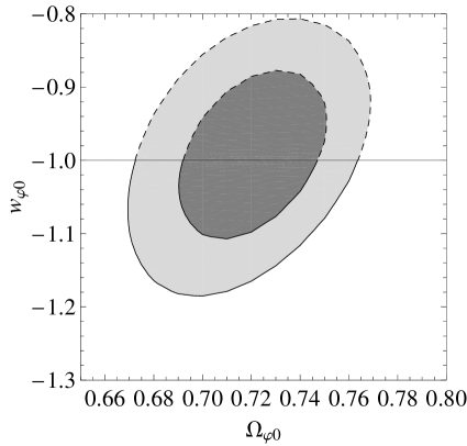
Figure 5: $1\sigma$ and $2\sigma$ confidence contours in the plane defined by the present-day values of $\Omega_{\phi}$ and $w_{\phi}$ (denoted by $\Omega_{\phi 0}$ and $w_{\phi 0}$ respectively). The dashed curves correspond to quintessence scenario while the solid curves to the phantom one. Note that the contours match exactly at the $w_{\phi 0}=-1$ line, although the corresponding fitting-expressions are not “symmetric” between the two cases.

We should mention that while fitting our model with the observational data, we have to do it separately for quintessence and phantom case, since the expressions for $(1+w_{\phi})$ and $-(1+w_{\phi})$ as a function of scale factor are not the same. This is unlike the minimally coupled case Scherrer:2007pu ; Scherrer:2008be , where they are exactly identical. In this regard, and from the fitting procedure point of view, one does not expect in general to have the confidence contours for quintessence and phantom case to match exactly to give a complete ellipse, simply because we are fitting two different $w_{\phi}(a)$. On the other hand, since we have switched the sign of the kinetic term of the scalar field in order to obtain the phantom model, we theoretically expect continuity for the exact solution and the contour to cross smoothly to the phantom region. Thus, the fact that the contours match exactly, as shown in fig. 5, indicates that our approximate method works well for both quintessence and phantom cases.

As we observe, and similarly to the minimally-coupled cases Scherrer:2007pu ; Scherrer:2008be ; amna , in order to acquire tight constraints on $w_{\phi 0}$ one has to impose strong bounds on $\Omega_{\phi 0}$, arising from the corresponding constraints on $\Omega_{m0}$ from structure formation data like the shape parameter for the matter power spectrum. However, with the present data, and although the behavior is richer than the minimally coupling scenarios, one cannot distinguish between the present model and a $\Lambda$CDM one.

IV Conclusions

In the present work we have studied dark energy scenarios in which the scalar field is non-minimally coupled to gravity and it evolves in nearly flat potentials in order for the slow-roll conditions to be satisfied. For completeness, we have investigated both quintessence and phantom cases in a unified way, having in mind that the later paradigm could have problems at the quantum level (the relevant discussion is still open in the literature since for instance in Cline:2003gs the authors reveal the causality and stability problems while in quantumphantom0 the authors construct a phantom theory consistent with the basic requirements of quantum field theory with the phantom fields arising as an effective description).

We have shown that all such models converge to a common behavior and we have extracted the corresponding approximate analytical expressions for $w_{\phi}(\Omega_{\phi})$ (relation (II)) and for $w_{\phi}(a)$ (relation (II)). The smallness of the non-minimal coupling parameter ($\xi=1/6$ in the conformal case) enhances the validity of our formulae, since it downgrades the role of the additional degree of freedom comparing to the minimal-coupling case. In particular, the errors are typically within $2\%$, and are smaller for $w_{\phi}$ being closer to $-1$ and for more flat potentials. Moreover, a comparison with observations using Baryon Acoustic Oscillation and latest Supernovae data reveals that the situation is similar to that of a minimally coupled scalar field. That is, under the present data the model cannot be distinguished from a $\Lambda$CDM scenario. However, one should note that in our investigation we have fixed the parameter $\xi$ to its conformal value $1/6$. Keeping $\xi$ arbitrary will make the parameter space broader, which in turn will lead further to less stringent constraints. In other words, switching on non-minimal coupling it becomes easier to fit the observational data, at least at the background cosmological level.

Non-minimal coupling leads to richer cosmological behavior comparing to the minimal scenario. For instance, although in minimal coupling with completely flat potentials one obtains the cosmological constant universe (i.e $w=-1=const.$) Scherrer:2007pu ; Scherrer:2008be , in the model at hand, even in this case one obtains a varying $w$ resulting purely from non-minimal coupling. In addition, it is interesting to see that non-minimal coupling introduces an “asymmetry” between quintessence and phantom cases, which is visible straightaway in the energy density and pressure definitions (5) and (6). However, even if the expressions are non-symmetric in the two sides of the phantom divide, the observation comparison reveals a non-trivial match of the confidence contours at the $w_{\phi 0}=-1$ line. This feature provides a physical self-consistency test of the obtained analytical expressions of the present work.

Finally, we mention that we have only considered observational data related to distance measurements, depending only on the background homogeneous and isotropic universe. An additional consideration of the growth of matter perturbations in these models, can have interesting effects and may help to distinguish between the present model and the cosmological-constant one. This will be our aim in a future investigation.

Acknowledgements:

ENS wishes to thank Institut de Physique Théorique, CEA, for the hospitality during the preparation of the present work. AAS acknowledges the financial support provided by the University Grants Commission, Govt. Of India through the major research project grant (Grant No:33-28/2007(SR)). AAS also knowledges the financial grant provided by the Theory Divison at CERN and the High Energy Physics Division at Abdus Salam International Center For Theoretical Physics, where part of the work has been done.

References

- (1) A. G. Riess et al., Astron. J. 116, 1009 (1998); S. Perlmutter et al., Astrophys. J. 517, 565 (1999); J. L. Tonry et al., Astrophys. J. 594, 1 (2003).
- (2) A. Melchiorri et al., Astrophys. J. Lett. 536, L63 (2000); A. E. Lange et al., Phys. Rev. D 63, 042001 (2001); A. H. Jaffe et al., Phys. Rev. Lett. 86, 3475 (2001); C. B. Netterfield et al., Astrophys. J. 571, 604 (2002); N. W. Halverson et al., Astrophys. J. 568, 38 (2002).
- (3) S. Bridle, O. Lahab, J. P. Ostriker and P. J. Steinhardt, Science 299, 1532 (2003); C. Bennett et al., Astrophys. J. Suppl. Ser. 148, 1 (2003); G. Hinshaw et al., Astrophys. J. Suppl. Ser. 148, 135 (2003); A. Kogut et al., Astrophys. J. Suppl. Ser. 148, 161 (2003); D. N. Spergel et al., Astrophys. J. Suppl. Ser. 148, 175 (2003).
- (4) P. Binétruy, C. Deffayet, D. Langlois, Nucl. Phys. B 565, 269 (2000); G.R. Dvali, G. Gabadadze, M. Porrati, Phys. Lett. B 485, 208 (2000); S. Capozziello, Int. J. Mod. Phys. D 11, 483 (2002); S.Nojiri and S. D. Odintsov, Phys. Rev. D 68, 123512 (2003); P. S. Apostolopoulos, N. Brouzakis, E. N. Saridakis and N. Tetradis, Phys. Rev. D 72, 044013 (2005); S.Nojiri and S. D. Odintsov, Int. J. Geom. Meth. Mod. Phys. 4, 115 (2007); F. K. Diakonos and E. N. Saridakis, JCAP 0902, 030 (2009); E. N. Saridakis, arXiv:0905.3532 [hep-th].
- (5) P. J. E. Peebles and B. Ratra, Astrophys. J. 325, L17 (1988); C. Wetterich, Nucl. Phys. B 302, 668 (1988); M. S. Turner and M. White, Phys. Rev. D 56, 4439 (1997); R. R. Caldwell, R. Dave and P. J. Steinhardt, Phys. Rev. Lett. 80, 1582 (1998); I. Zlatev, L. M. Wang and P. J. Steinhardt, Phys. Rev. Lett. 82, 896 (1999); A. J. Albrecht, C. P. Burgess, F. Ravndal and C. Skordis, Phys. Rev. D 65, 123507 (2002); M. Sahlen, A. R. Liddle and D. Parkinson, Phys. Rev. D 72, 083511 (2005); M. Sahlen, A. R. Liddle and D. Parkinson, Phys. Rev. D 75, 023502 (2007); D. Huterer and H. V. Peiris, Phys. Rev. D 75, 083503 (2007); Z. K. Guo, N. Ohta and Y. Z. Zhang, Mod. Phys. Lett. A 22, 883 (2007); S. Dutta, E. N. Saridakis and R. J. Scherrer, Phys. Rev. D 79, 103005 (2009) [arXiv:0903.3412 [astro-ph.CO]].
- (6) R. R. Caldwell, Phys. Lett. B 545, 23 (2002); R. R. Caldwell, M. Kamionkowski and N. N. Weinberg, Phys. Rev. Lett. 91, 071301 (2003); P. F. Gonzalez-Diaz and C. L. Siguenza, Nucl. Phys. B 697, 363 (2004); S. Nojiri and S. D. Odintsov, Phys. Rev. D 72, 023003 (2005); H. Garcia-Compean, G. Garcia-Jimenez, O. Obregon, and C. Ramirez, JCAP 0807, 016 (2008); X. m. Chen, Y. g. Gong and E. N. Saridakis, JCAP 0904, 001 (2009); E. N. Saridakis, Nucl. Phys. B 819, 116 (2009).
- (7) B. Feng, X. L. Wang and X. M. Zhang, Phys. Lett. B 607, 35 (2005); Z. K. Guo, et al., Phys. Lett. B 608, 177 (2005); M.-Z Li, B. Feng, X.-M Zhang, JCAP, 0512, 002 (2005); Y. f. Cai, H. Li, Y. S. Piao and X. m. Zhang, Phys. Lett. B 646, 141 (2007); W. Zhao and Y. Zhang, Phys. Rev. D 73, 123509 (2006); M. R. Setare and E. N. Saridakis, Phys. Lett. B 668, 177 (2008); M. R. Setare and E. N. Saridakis, JCAP 0809, 026 (2008).
- (8) K. Griest, Phys. Rev. D66, 123501 (2002); S. Bludman, Phys. Rev. D69, 122002 (2004); R.R. Caldwell and E.V. Linder, Phys. Rev. Lett. 95, 141301 (2005); E.V. Linder, Phys. Rev. D73, 063010 (2006); S. Chongchitnan and G. Efstathiou, Phys. Rev. D76, 043508 (2007).
- (9) J. Kujat, R. J. Scherrer and A. A. Sen, Phys. Rev. D 74, 083501 (2006).
- (10) Q. G. Huang, Phys. Rev. D 77, 103518 (2008); E. N. Saridakis, Phys. Lett. B 676, 7 (2009).
- (11) R. J. Scherrer and A. A. Sen, Phys. Rev. D 77, 083515 (2008).
- (12) R. J. Scherrer and A. A. Sen, Phys. Rev. D 78, 067303 (2008).
- (13) M. R. Setare and E. N. Saridakis, Phys. Rev. D 79, 043005 (2009).
- (14) A. Ali, M. Sami and A. A. Sen, arXiv:0904.1070 [astro-ph.CO].
- (15) V. Sahni and S. Habib, Phys. Rev. Lett. 81, 1766 (1998); J. P. Uzan, Phys. Rev. D 59, 123510 (1999); A. A. Sen and S. Sen, Mod. Phys. Lett. A 16, 1303 (2001); S. Sen and A. A. Sen, Phys. Rev. D 63, 124006 (2001); T. Chiba, Phys. Rev. D 60, 083508 (1999); F. Perrotta, C. Baccigalupi and S. Matarrese, Phys. Rev. D 61, 023507 (2000); E. Elizalde, S. Nojiri and S. Odintsov, Phys. Rev. D 70, 043539 (2004); V. K. Onemli and R. P. Woodard, Phys. Rev. D 70, 107301 (2004); E. Elizalde et al, Phys. Rev. D 77, 106005 (2008).
- (16) V. Faraoni, Phys. Rev. D 68, 063508 (2003); S. Nojiri, S. D. Odintsov and M. Sami, Phys. Rev. D 74, 046004 (2006); M. Szydlowski, O. Hrycyna and A. Kurek, Phys. Rev. D 77, 027302 (2008); O. Hrycyna, M. Szydlowski, Phys. Rev. D 76, 123510 (2007); M. R. Setare and E. N. Saridakis, Phys. Lett. B 671, 331 (2009); M. R. Setare and E. N. Saridakis, JCAP 0903, 002 (2009).
- (17) A. R. Liddle and R. J. Scherrer, Phys. Rev. D 59, 023509 (1998); V. Faraoni, Phys. Rev. D 62, 023504 (2000); N. Bartolo and M. Pietroni, Phys. Rev. D 61, 023518 (2000); O. Bertolami and P. J. Martins, Phys. Rev. D 61, 064007 (2000); R. de Ritis, A. A. Marino, C. Rubano and P. Scudellaro, Phys. Rev. D. 62, 043506 (2000); T.D. Saini, S. Raychaudhury, V. Sahni and A. A. Starobinsky, Phys. Rev. Lett. 85, 1162 (2000); S. Sen and T. R. Seshadri, Int. J. Mod. Phys. D 12, 445 (2003).
- (18) A. A. Sen, G. Gupta and S. Das, arXiv:0901.0173 [astro-ph.CO].
- (19) P.G. Ferreira, M. Joyce, Phys. Rev. Lett. 79, 4740 (1997); E. J. Copeland, A. R. Liddle and D. Wands, Phys. Rev. D 57, 4686 (1998).
- (20) M. Szydlowski and O. Hrycyna, JCAP 0901, 039 (2009).
- (21) M. Sami, A. Toporensky, Mod. Phys. Lett. A 19, 1509 (2004).
- (22) M. Kowalski et.al, Astrophys. J. 686, 749 (2008).
- (23) D. J. Eisenstein et.al, Astrophys. J. 633, 560 (2005).
- (24) J. M. Cline, S. Jeon and G. D. Moore, Phys. Rev. D 70, 043543 (2004).
- (25) S. Nojiri and S. D. Odintsov, Phys. Lett. B 562, 147 (2003); S. Nojiri and S. D. Odintsov, Phys. Lett. B 571, 1 (2003).