DNA looping provides stability and robustness to the bacteriophage $\lambda$ switch

Abstract

The bistable gene regulatory switch controlling the transition from lysogeny to lysis in bacteriophage $\lambda$ presents a unique challenge to quantitative modeling. Despite extensive characterization of this regulatory network, the origin of the extreme stability of the lysogenic state remains unclear. We have constructed a stochastic model for this switch. Using Forward Flux Sampling simulations, we show that this model predicts an extremely low rate of spontaneous prophage induction in a recA mutant, in agreement with experimental observations. In our model, the DNA loop formed by octamerization of CI bound to the $O_{L}$ and $O_{R}$ operator regions is crucial for stability, allowing the lysogenic state to remain stable even when a large fraction of the total CI is depleted by nonspecific binding to genomic DNA. DNA looping also ensures that the switch is robust to mutations in the order of the $O_{R}$ binding sites. Our results suggest that DNA looping can provide a mechanism to maintain a stable lysogenic state in the face of a range of challenges including noisy gene expression, nonspecific DNA binding and operator site mutations.

The bistable developmental switch controlling the transition from lysogeny to lysis in bacteriophage $\lambda$ is one of the best characterized gene regulatory networks lphagebook . In the lysogenic state, the phage $\lambda$ genome is integrated into the chromosome of the Escherichia coli host cell and is essentially dormant, due to expression of the $cI$ repressor gene, the product of which represses $cro$ and other genes (Fig. 1). A transition to the lytic switch state can occur in response to DNA damage (via UV irradiation), when CI molecules are cleaved by RecA. Transcription of the $cro$ gene from $P_{R}$ then triggers a cascade of gene activation, leading to phage excision, replication and cell lysis. In mutants where this cascade is blocked, a state with elevated Cro levels is stable for several cell generations. This is known as the anti-immune state Calef . A simple and intuitive explanation has been presented for this bistability lphagebook : in the lysogenic state, CI is dominant and $cro$ is repressed; yet, once $cro$ begins to be expressed, Cro dimers repress transcription of $cI$, making the transition to lysis inevitable. However, quantitative measurements have revealed a puzzle: the lysogenic state of the phage $\lambda$ switch is both extremely stable Little99 ; Aurell02 ; Rozanov98 and robust to rewiring of its transcriptional regulatory interactions Little99 . These features have not yet been explained by mathematical models. Here, we present dynamical simulations of a stochastic mathematical model that reproduces this seemingly mysterious behavior. Our simulations provide evidence that DNA looping plays a key role in ensuring the stability and robustness of the switch.

The molecular interactions controlling the transcription of $cI$ and $cro$ have been studied in great detail. CI and Cro bind as dimers to the operator sites $O_{R}1$, $O_{R}2$ and $O_{R}3$ (Figure 1), which control expression of the cI and cro genes from the $P_{RM}$ and $P_{R}$ promoters. Transcription from the unactivated $P_{RM}$ promoter is about 10 times weaker than from $P_{R}$; however, when a CI dimer is bound at $O_{R}2$, transcription from $P_{RM}$ is enhanced to about the same level as from $P_{R}$ (i.e. the two promoters can compete with one another only when CI is bound at $O_{R}2$). CI dimers bind preferentially and co-operatively to the $O_{R}1$ and $O_{R}2$ sites, which overlap the $P_{R}$ promoter. When CI is bound to these two sites, $cro$ ($P_{R}$) is repressed and $cI$ ($P_{RM}$) is activated. Cro dimers bind preferentially to $O_{R}3$, which overlaps $P_{RM}$, so that when this site is occupied, $cI$ is repressed lphagebook . An important additional component of the network architecture is a DNA loop which can form between the $O_{R}$ site and the left operator site $O_{L}$, located 2400bp from $O_{R}$, which also has three adjacent binding sites for CI dimers ($O_{L}1$, $O_{L}2$ and $O_{L}3$). The loop is mediated by octamerization between pairs of CI dimers bound at $O_{R}$ and $O_{L}$ Revet99 . The role of this DNA looping interaction in the function of the phage $\lambda$ switch remains a subject of debate Dodd01 ; Dodd04 ; Svenningsen05 ; roma ; anderson2008 .

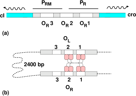
Figure 1: Schematic illustration of (a): the $O_{R}$ region of the phage $\lambda$ switch, and (b): the DNA loop formed by octamerization of CI dimers bound of $O_{R}$ and $O_{L}$.

Quantitative measurements have revealed several intriguing features of the phage $\lambda$ switch. Firstly, the lysogenic state is extremely stable Little99 ; Aurell02 ; Rozanov98 , despite the stochastic nature of the underlying gene regulatory network Stochastic fluctuations in gene regulation (“noise”) might be expected to cause spontaneous transitions from the lysogenic to lytic states, even in lysogens lacking RecA; yet the rate of these transitions is so low as to be almost unmeasurable. Secondly, recent measurements of $P_{RM}$ and $P_{R}$ promoter activity suggest that only a small fraction of the total CI in the cell is available for binding to $O_{R}$ Dodd01 ; Dodd04 ; Reinitz90 ; Pakula86 ; Bakk04_1 , while other measurements show that the total concentration of CI in the lysogen varies dramatically from cell to cell Baek03 . Taken together, these results suggest that the stability of the lysogen is rather insensitive to the number of free intracellular CI molecules. Despite this stability, transition to lysis occurs readily in wild-type phage on UV irradiation, which leads to cleavage of CI by RecA. Finally, and remarkably, switch function is robust to changes in the gene network architecture itself: when the order of the three $O_{R}$ binding sites is altered so that $O_{R}1$ is replaced by $O_{R}3$ or vice versa, the network remains functional Little99 .

Computer simulations should be an excellent tool for explaining this behavior. Although stochastic simulations have successfully been used to model the initial developmental choice between lysogeny and lysis for lambda-infected cells arkin1998 , modelling spontaneous switching of an already established lysogen has proved problematic. Despite the fact that a wealth of biochemical parameters are available for this network, no model has reproduced its extraordinary stability and functional robustness Aurell02 ; Reinitz90 ; AS ; Tian04 ; Lou07 ; Zhu04 ; Santillan04 . In this paper, we present a model that takes into account the stochastic character of the chemical reactions and includes DNA looping and depletion of free CI and Cro by nonspecific binding to genomic DNA. Our model also explicitly describes the detailed dynamics of the binding of transcription factors to the promoters. Accurate computation of spontaneous switching rates for this large reaction set is achieved using the Forward Flux Sampling (FFS) rare event simulation method Allen05 ; Allen06_1 , in combination with temporal coarse-graining of dimerization and nonspecific DNA binding reactions. Our simulations show that this stochastic model can reproduce the bistability of the switch and its robustness to operator site mutations, as well as the extreme stability of the lysogenic state, even in the presence of nonspecific DNA binding.

In this work, we study the effect on switch function of two key parameters: the strengths of the DNA looping and nonspecific binding interactions. We find that the DNA looping interaction plays a crucial role. In the absence of the looping interaction, a highly stable lysogenic state can be achieved, but this state is very sensitive to depletion of free CI and to operator site mutations. When looping is included in the model, the lysogen is insensitive to CI depletion and robust to rearrangement of the operator sites. We conclude that DNA looping may play an important role in allowing the phage $\lambda$ switch to function reliably even under highly destabilizing conditions in the host cell.

I The model

Our model consists of a set of chemical reactions, simulated using the Gillespie algorithm Gillespie76 . The components of the model are: dimerization of CI and Cro proteins, binding of CI and Cro dimers to specific DNA binding sites $O_{R}1$, $O_{R}2$, $O_{R}3$, $O_{L}1$, $O_{L}2$ and $O_{L}3$, binding of RNA polymerase (RNAp) to promoters $P_{RM}$, $P_{R}$ and $P_{L}$, transcription of cI and cro, translation of the corresponding mRNA transcripts, degradation of mRNA transcripts and removal of CI and Cro monomers and dimers from the cell. Our model also includes formation of a DNA loop between $O_{R}$ and $O_{L}$, mediated by a CI octamer, and nonspecific binding of CI and Cro dimers to genomic DNA. The key parameters that we vary are the strength of the nonspecific DNA binding interaction $\Delta G_{\textrm{NSB}}$ and the strength of the DNA looping interaction $\Delta G_{\textrm{loop}}$. Other parameters are fixed using biochemical data as far as possible. The model parameters are discussed briefly here and described in full in the Supporting Information.

I.1 Host cell parameters

We assume that the E. coli host cell is growing rapidly (doubling time 34 min Little99 ), and has 3 copies of the $O_{R}$ and $O_{L}$ operators Aurell02 , in a cell volume of 2$\textrm{$\mu$m}^{3}$ Aurell02 . The concentration of free RNAp in the cytoplasm is taken to be 50nM mcclure1983_proc , but our conclusions are not sensitive to this parameter, as we demonstrate in the Supporting Information.

I.2 Operator binding dynamics

Equilibrium constants from the literature were used for CI Koblan92 ; Burz94_1 and Cro Darling00 binding to $O_{R}1$, $O_{R}2$, $O_{R}3$, for RNAp binding to $P_{RM}$ and $P_{R}$ Shea85 and for CI binding to the $O_{L}$ sites Dodd04 . Cro is assumed to bind to $O_{L}$ and $O_{R}$ sites identically. The total number of possible (unlooped) configurations of the $O_{R}$ and $O_{L}$ operators are, respectively, 40 and 36. Since we are performing dynamical simulations, we require rate constants $k_{a}$ and $k_{d}$ for association and dissociation. For all association rates, we used the diffusion-limited value $k_{a}=4\pi D\sigma=0.314\textrm{$\mu$m}^{3}\textrm{s}^{-1}$ (taking the diffusion constant $D=5\textrm{$\mu$m}^{2}\textrm{s}^{-1}$ and the molecular size $\sigma=5\textrm{nm}$). The rate constant for dissociation, in $\textrm{s}^{-1}$, was then deduced from the equilibrium constant, using $k_{a}/k_{d}=(\exp{[-\Delta G/RT]})/(6.023\times 10^{8})\textrm{$\mu$m}^{3}$, where $k_{a}$ is in $\textrm{$\mu$m}^{3}\textrm{s}^{-1}$, $\Delta G$ is in kcal/mol, $RT=0.616\textrm{kcal/mol}$ at 37C, and $6.023\times 10^{8}\textrm{$\mu$m}^{3}$ is a volume conversion factor.

I.3 Protein and mRNA production and removal

We model transcription as a single reaction in which an mRNA molecule is produced when RNAp is bound to a promoter. $P_{RM}$ activity is enhanced when a CI dimer is bound at $O_{R}2$. Transcription rates are 0.014$\textrm{s}^{-1}$ for $P_{R}$, 0.001$\textrm{s}^{-1}$ for unstimulated $P_{RM}$ and 0.011$\textrm{s}^{-1}$ for stimulated $P_{RM}$ Shea85 ; McClure82 ; Hwang88 ; Li97 . All mRNA transcripts are degraded with a half-life of 2 mins. Translation and protein folding are combined into a single step. The model produces a statistical distribution for the number of proteins produced per transcript, which is governed by the balance betwen the translation and mRNA degradation rates. The average of this distribution (the “burst size”) is 6 and 20 for CI and Cro respectively. The burst size for Cro follows ref. Aurell02 . The value for CI is based on the observation that the CI ribosome binding site (RBS) is $\sim 7$-fold weaker than that of LacZ dodd_pc , and that the LacZ burst size is 30-40 kennell ; sorensen . A somewhat weaker CI RBS was observed by Shean and Gottesman Shean92 . Protein monomers and dimers are removed with rate constant $\ln(2)/T$, where the cell cycle time $T=$34min Little99 . We also include active degradation of Cro monomers with half-life 42min Pakula86 ; Aurell02 .

I.4 Dimerization

Dimerization free energies are taken to be $-11\textrm{kcal/mol}$ for CI Burz94 ; Beckett91 and $-8.7\textrm{kcal/mol}$ for Cro Darling00_1 . The association reaction is again assumed to be diffusion-limited. To increase the efficiency of our simulations, we coarse-grain the monomer-monomer association and dissociation reactions for both CI and Cro morelli2008 , as described in the Supporting Information.

I.5 DNA looping

When an $O_{R}$ and an $O_{L}$ operator each carry at least two adjacent CI dimers (at the 1-2 or 2-3 sites), these operators can associate to form a “looped state”, with rate $k_{\textrm{loop}}$, which dissociates with rate $k_{\textrm{unloop}}$. The total number of possible looped states is 49. Binding of CI dimers to the two non-octamerized sites in a loop occurs with a cooperativity factor $\exp{[-\Delta G_{\textrm{tet}}/RT]}$ where $\Delta G_{\textrm{tet}}=-3\textrm{kcal/mol}$ Dodd04 . Because we assume fast growth of the host cell, our model contains 3 copies of the host genome and 3 copies of the phage $\lambda$ switch. Since the loop is much longer than the persistence length of DNA, we assume that any $O_{R}-O_{L}$ combination can form a loop. The strength and dynamics of the DNA loop in vivo are unknown. We therefore test the effects of DNA looping on the network behavior, by varying the ratio $k_{\textrm{loop}}/k_{\textrm{unloop}}\equiv\exp{[-\Delta G_{\textrm{loop}}/RT]}$. We generally assume a fixed value $62.1\textrm{s}^{-1}$ for $k_{\textrm{loop}}$ (arising from considerations of polymer dynamics as discussed in the Supporting Information), but we find that only the ratio is important.

I.6 Nonspecific DNA binding dynamics

We model nonspecific DNA binding Dodd04 ; Bakk04_1 by including in our reaction set association and dissociation of CI and Cro dimers to $10^{7}$ genomic DNA sites, corresponding to 2-3 copies of the bacterial genome. The association rate $k_{a}$ is assumed to be diffusion-limited, and we assume identical nonspecific binding affinities for CI and Cro. Nonspecifically bound dimers are removed from the cell with rate constant $\ln(2)/T$. We do not model nonspecific binding of RNAp, since our value of 50nM corresponds to the free RNAp concentration mcclure1983_proc . To investigate the effects of nonspecific DNA binding on the model switch, we vary the parameter $\Delta G_{\textrm{NSB}}$ where $k_{a}/k_{d}=(\exp{[-\Delta G_{\textrm{NSB}}/RT]})/(6.023\times 10^{8})\textrm{$\mu$m}^{3}$. We assume that these reactions are fast compared to the other reactions in the network, and can be coarse-grained morelli2008 as described in the Supporting Information.

II Bistability

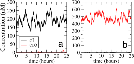
Figure 2: The model switch is bistable. Typical simulation trajectories are shown for $\Delta G_{\textrm{loop}}=-3.7\textrm{kcal/mol}$ and $\Delta G_{\textrm{NSB}}=-4.1\textrm{kcal/mol}$. (a): A simulation initiated with 150nM CI and no Cro molecules remains in the CI-rich state for many hours (b): A simulation initiated with 400nM Cro and no CI molecules remains in the Cro-rich state.

Our model represents a mutant phage in which the lytic pathway is nonfunctional, since we do not model the lytic genes downstream of cro Calef . Such mutants show two stable states: the very stable lysogenic state, with high CI and low Cro levels, and the anti-immune state, with elevated Cro and little CI, which is less stable, but is nevertheless maintained for several generations Calef . For our model to reproduce this bistability, simulations initiated in either of the lysogenic or anti-immune states should remain stable, only rarely making a spontaneous transition to the other state. Figure 2 shows that this is indeed the case: in Figure 2a, a simulation initiated in the lysogenic state remains in that state, while in Figure 2b, a simulation run with the same parameters but initiated with a high Cro concentration and little CI remains in the anti-immune state. Figure 3 shows the range of parameter values for which our model shows bistability. Our simulations give steady state concentrations of CI and Cro in good agreement with measured values for the lysogenic and anti-immune states. For the lysogenic state, we obtain $\sim 200-400$ CI per cell, compared to a measured value of 220 Reichardt71 . For the anti-immune state, Cro per cell ranges from $\sim 250-900$ (depending on $\Delta G_{\textrm{NSB}}$), corresponding to concentrations of $200-750\textrm{nM}$, compared to a measured concentration of $\sim 400\textrm{nM}$ Reinitz90 . These values are presented as functions of $\Delta G_{\textrm{loop}}$ and $\Delta G_{\textrm{NSB}}$ in the Supporting Information. In our model, the DNA looping interaction decreases the lysogenic CI concentration by as much as a factor of 2, in agreement with the observations of Dodd et al Dodd01 ; Dodd04 . We have also simulated mutants without the $O_{R}3$ or the $O_{L}3$ binding sites, corresponding approximately to the OR3-r1 and OL3-4 mutants of refs Dodd01 , Dodd04 and anderson2008 . For these mutants, we find lysogenic CI concentrations 1.9 and 1.8 times the wild-type values (for $\Delta G_{\textrm{loop}}=-3.7\textrm{kcal/mol}$ and $\Delta G_{\textrm{NSB}}=-2.8\textrm{kcal/mol}$), in reasonable agreement with the results of ref Dodd04 (factors of 2.8 and 3 respectively), even though our model does not include the up-regulation of $P_{RM}$ by the loop identified in ref anderson2008 , or the effect on $P_{RM}$ of the OR3-r1 mutation. For the same parameters, the $P_{R}$ promoter is repressed by a factor of $1.6$ in the anti-immune state, in good agreement with ref. Svenningsen05 .

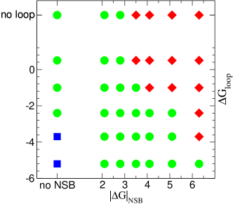
Figure 3: Bistability of the model switch as a function of the nonspecific binding strength $\Delta G_{\textrm{NSB}}$ and the DNA looping strength $\Delta G_{\textrm{loop}}$. Blue squares represent parameter sets for which only the lysogenic state is stable (no stable anti-immune state); for red diamonds only the anti-immune state is stable (no stable lysogen), while green circles represent parameter combinations where the model switch is bistable.

III Extreme stability of the lysogenic state

The spontaneous switching rate from lysogeny to lysis in recA– mutants is so low as to be almost undetectable, being less than $2\times 10^{-9}$ per cell per generation Little99 ; Aurell02 . Reproducing such low spontaneous switching rates while maintaining bistability provides an extreme challenge for a computational model Aurell02 . We quantified the stability of the lysogenic and anti-immune states for our model, using the forward flux sampling (FFS) rare event simulation method Allen05 ; Allen06_1 . This method allows us to compute the rate of spontaneous switch flips, even though such flips would hardly ever be observed in a typical “brute-force” simulation run. FFS uses a series of interfaces (defined by an order parameter) between the initial (CI-rich) and final (Cro-rich) states to split a switching event into a number of more likely transitions between successive interfaces. Here, our order parameter was the difference between the total number of Cro and CI molecules. This method has previously been used for a simple model of a mutually repressing genetic switch Allen05 ; Allen06_1 . Details of the FFS method and its implementation are given in the Supporting Information.

Our results are listed in Table 1. In the absence of DNA looping (top two rows of Table 1), the lysogen is stable for $\sim 10^{9}$ generations only when nonspecific DNA binding is absent. When nonspecific binding is included in the model, the lysogen becomes much less stable: a relatively modest nonspecific binding strength $\Delta G_{\textrm{NSB}}=-2.1\textrm{kcal/mol}$ produces a lysogen that is only stable for $\sim 1700$ generations: approximately a million times less stable than the experimental lower bound. In contrast, when DNA looping is included in the model (bottom three rows of Table 1), extremely stable lysogens can be achieved for a wide range of DNA looping and nonspecific DNA binding strengths. These lysogenic states are in fact even more stable than those observed experimentally Little99 . One possible explanation might be the effects of passing DNA replication forks (not included in the model), which might be expected to destabilize looped DNA configurations and/or remove bound CI from the operator sites. The anti-immune state for our model is much less stable than the lysogenic state, in agreement with experimental observations Calef ; Svenningsen05 .

Table 1: Spontaneous switching times (inverse of calculated switching rates) from the lysogenic to anti-immune states and from the anti-immune to lysogenic states, for wild-type phage $\lambda$, computed using FFS.

$\Delta G_{\textrm{loop}}$	$\Delta G_{\textrm{NSB}}$	Switching time	Switching time
kcal/mol	kcal/mol	lysogen $\to$ anti-immune	anti-immune $\to$ lysogen
		(generations)	(generations)
no loop	no NSB	$(3.6\pm 0.1)\times 10^{9}$	$2300\pm 100$
no loop	-2.8	$1700\pm 50$	$(7\pm 1)\times 10^{9}$
-5.2	-4.1	$<10^{23}$	$43\pm 1$
-3.7	-2.8	$(3\pm 2)\times 10^{25}$	$26\pm 1$
-1.0	no NSB	$(6\pm 2)\times 10^{14}$	$130\pm 10$

IV DNA looping allows the switch to function despite CI depletion

It is believed that a large fraction of the transcription factors in a bacterial cell are unavailable for binding to their specific binding sites because they are nonspecifically bound to genomic DNA Hippel74 . Recent expression measurements for the $P_{RM}$ promoter have suggested that this is the case for CI Dodd01 ; Dodd04 ; Bakk04_1 . This nonspecific binding poses a severe challenge to the phage $\lambda$ switch. Although both CI and Cro are depleted by nonspecific binding, the $P_{RM}$ promoter is intrinsically weak, and requires activation by CI at $O_{R}2$ to compete effectively with $P_{R}$. One would therefore expect nonspecific DNA binding by CI to drastically destabilize the lysogen, and to compromise the bistability of the switch. Table 2 of the Supporting Information shows how the concentration of free CI depends on the nonspecific DNA binding strength. To characterise the effects on switch function, we investigated the range of nonspecific binding strengths over which our model gave bistability, for different values of the DNA looping parameter $\Delta G_{\textrm{loop}}$. Our results are shown in Figure 3. In the absence of DNA looping (top row of Figure 3), bistability is indeed strongly compromised as the parameter $\Delta G_{\textrm{NSB}}$ is increased in magnitude (left to right). For $|\Delta G_{\textrm{NSB}}|>\sim 3\textrm{kcal/mol}$, the model is no longer bistable; the lysogenic state cannot be sustained and only the anti-immune state is stable. However, when the DNA looping interaction is included in the model, bistability is maintained over a much wider range of $\Delta G_{\textrm{NSB}}$ values. In figure 3, the width of the green (bistable) region increases dramatically as the parameter $|\Delta G_{\textrm{loop}}|$ increases. Our model therefore suggests that one role of the DNA looping interaction may be to ensure that the switch continues to function even when the level of intracellular free CI is depleted by nonspecific DNA binding Dodd01 ; Dodd04 or by cell-to-cell fluctuations Baek03 . We note that this stability to CI fluctuations is not expected to prevent lysis from occurring on UV irradiation of the wild-type phage: even for a strong looping interaction, rapid degradation of CI by RecA will eventually lead to so little CI being present that the loop cannot be maintained, upon which lysis will occur. To check this, we simulated a version of the model in which we fixed the total CI concentration, for a typical parameter set ($\Delta G_{\textrm{loop}}=-3.7\textrm{kcal/mol}$, $\Delta G_{\textrm{NSB}}=-2.8\textrm{kcal/mol}$). When we artificially lower the CI concentration to $\sim 10\%$ of the lysogenic steady-state level (30 CI molecules per cell), the system flips to the anti-immune state. This result is in good agreement with the observation of Bailone et al Bailone1979 that prophage induction occurs at a CI concentration about 10$\%$ of that in the lysogen.

V DNA looping causes robustness to operator mutations

In an important series of experiments, Little et al showed that the basic functions of the phage $\lambda$ regulatory network are robust to changes in network architecture. Mutants $O_{R}(121)$ and $O_{R}(323)$, in which the order of the $O_{R}1$, $O_{R}2$ and $O_{R}3$ binding sites was altered compared to the wild-type $O_{R}(321)$, formed stable lysogens (although less stable than the wild-type) which could be induced to enter the lytic pathway on UV irradiation Little99 . To our knowledge, this robustness has not been reproduced in computer models Aurell02 .

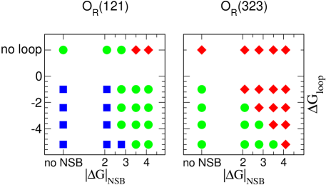
Figure 4: Range of bistability of the model switch as a function of the nonspecific DNA binding parameters $\Delta G_{\textrm{NSB}}$ and $\Delta G_{\textrm{loop}}$, in the presence and absence of the DNA looping interaction, for the Little mutants. Symbols have the same meaning as in Figure 3.

We tested whether our model was able to produce stable lysogens for the $O_{R}(121)$ and $O_{R}(323)$ mutants, which were created in our simulations by changing the operator binding site affinities. We neglect possible changes in the properties of $P_{RM}$ hammer2006 , whose DNA sequence is also affected by the Little et al substitutions. The range of parameters for which our model mutants are bistable is shown in Figure 4. We find that the DNA looping interaction plays a key role in ensuring robustness. In the absence of DNA looping (top row of Figure 4), our model produces a stable lysogen for $O_{R}(121)$ only if the nonspecific binding strength $\Delta G_{\textrm{NSB}}$ is below a critical value, and cannot sustain a stable lysogen for $O_{R}(323)$ at all. However, when DNA looping is included in the model (lower rows of Figure 4), the $O_{R}(323)$ mutant can achieve a stable lysogenic state, and the $O_{R}(121)$ lysogen becomes able to tolerate stronger nonspecific DNA binding interactions. In fact, if the looping strength is too strong, our model predicts that the $O_{R}(121)$ mutant may lose the ability to sustain a stable anti-immune state.

The steady-state concentrations of CI in the lysogen predicted for these mutants are in reasonable agreement with the observations of Little et al. For a typical parameter set ($\Delta G_{\textrm{loop}}=-3.7\textrm{kcal/mol}$, $\Delta G_{\textrm{NSB}}=-2.8\textrm{kcal/mol}$), we obtained steady-state lysogenic CI concentrations $38\%$ and $81\%$ of the wild-type values for $O_{R}(121)$ and $O_{R}(323)$ respectively, in comparison to $25$–$30\%$ and $60$–$75\%$ measured by Little et al. Calculation of the spontaneous switching rates for the $O_{R}(121)$ and $O_{R}(323)$ mutants, using FFS, also shows results qualitatively in agreement with those of Little et al Little99 (see table of results in the Supporting Information). For all combinations of $\Delta G_{\textrm{loop}}$ and $\Delta G_{\textrm{NSB}}$, the $O_{R}(323)$ lysogen is less stable than $O_{R}(121)$ which is in turn less stable than the wild-type, although quantitatively the magnitude of this destabilization is greater than the factors of 10 observed by Little et al. Our model allows us to make the tentative prediction that (in a $recA$– host) the stability of the anti-immune states will be $O_{R}(323)>$ wild-type $>O_{R}(121)$. These stabilities have not yet been measured littlepc .

VI Alternatives to looping

Our results indicate that the DNA looping interaction allows the phage $\lambda$ switch to maintain an extremely stable lysogenic state, which is robust to operator mutations, while retaining its essential bistability. Could this result have been achieved by evolution in any other way? Recent work by Babić and Little Babic07 has shown that a triple mutant lacking CI cooperativity but with increased $P_{RM}$ activity and enhanced binding of CI to $O_{R}2$, can maintain a stable lysogen, with increased CI levels compared to the wild-type, and can switch into the lytic state. It is very unlikely that this mutant can form a DNA loop littlepc . This suggests that increased lysogenic CI levels could substitute for cooperative interactions (including DNA looping). To test whether our model could reproduce these experiments, we modified our simulation parameters to represent the two triple mutants $\lambda$ $cI$ Y210N prm252 $O_{R}2up$ and $\lambda$ $cI$ Y210N prmup-1 $O_{R}2up$. In both cases, we removed all cooperative interactions between CI dimers, including looping, and increased the affinity of CI for $O_{R}2$ by a factor of 5. For the prm252 mutation, the basal and stimulated $P_{RM}$ transcription rates were increased by factors of 6 and 2.5 respectively, and for the prmup-1 mutation these factors were 10 and 5 Babic07 . With nonspecific binding strength $\Delta G_{\textrm{NSB}}=-2.1\textrm{kcal/mol}$, both these “mutants” formed stable lysogens, with CI levels $\sim 3$ and $\sim 6$ times that of the “wild-type”. The mutant representing $\lambda$ $cI$ Y210N prmup-1 $O_{R}2up$ also formed a stable lysogen for $\Delta G_{\textrm{NSB}}=-2.8\textrm{kcal/mol}$, but $\lambda$ $cI$ Y210N prm252 $O_{R}2up$ did not. These results are in reasonable agreement with those reported by Babić and Little Babic07 . Furthermore, our results support the view that increased lysogenic CI levels could provide an alternative mechanism for maintaining a stable lysogenic state, although this mechanism has apparently not been selected by evolution.

VII Discussion

The phage $\lambda$ switch represents an important test for computational modeling of gene regulatory networks. This network has been a paradigm in molecular biology for many years: its architecture and biochemical parameters have been extensively studied and its behavior has been thoroughly and quantitatively characterized. Nevertheless, computational models have failed to produce results in agreement with experimental observations. If modeling is to prove a useful tool in the analysis of larger and more complex gene regulatory networks, it is essential that it should produce convincing results for phage $\lambda$.

The computer simulation model presented here reproduces for the first time both the bistability of the phage $\lambda$ switch and its extremely low spontaneous flipping rate. Our model includes only known biochemical interactions and uses as far as possible biochemically measured parameters. The forward flux sampling (FFS) rare event sampling method allows us to quantify the stability of the lysogenic and anti-immune states, even though spontaneous switching rates would never be observed in a typical brute-force simulation run. An important difference between our model and previous theoretical studies is that we simulate the full transcription factor-DNA binding dynamics. These “operator state fluctuations” were eliminated in previous models, using the physical-chemical quasi-equilibrium assumption of Shea and Ackers Aurell02 ; Santillan04 ; Shea85 . Our previous work Morelli2008_2 , as well as that of Walczak and Wolynes Walczak05 , has shown that operator state fluctuations can drastically affect the switching pathways and the switching rate for bistable genetic networks. Moreover, Vilar and Leibler Vilar03 have shown that operator state fluctuations are coupled to DNA looping dynamics. We therefore model explicitly both the protein-DNA binding dynamics and the DNA looping dynamics. Our model also includes nonspecific DNA binding, as does ref. Aurell02 . Although DNA looping and nonspecific binding are modeled in a simplified manner, our model involves many reactions and is computationally expensive to simulate. This problem is alleviated by the FFS method, in combination with the coarse-graining of dimerization and non-specific binding reactions. We note that a semi-analytical approach, based on Large Deviation Theory, which has been applied successfully to a simplified model of the phage $\lambda$ switch roma , may provide a promising alternative to direct simulations as performed here.

Our results suggest a key role for the DNA looping interaction in ensuring that the network retains its bistability even when exposed to perturbations. Our model requires DNA looping to achieve bistability in the presence of nonspecific DNA binding and/or operator state mutations. The $P_{RM}$ promoter is intrinsically weak and requires CI to be bound at $O_{R}2$ in order to compete effectively with $P_{R}$. The DNA loop enhances CI occupancy at $O_{R}2$, providing a way to achieve sustained activation of the $P_{RM}$ promoter, even when the free intracellular CI concentration is very small. We also find, in agreement with Dodd et al, that the presence of the loop increases autorepression of $P_{RM}$ by enhancing CI binding at $O_{R}3$ Dodd01 . Looping thus increases the strength of both auto-activation via $O_{R}2$ and auto-repression via $O_{R}3$; this reduces the fluctuations in CI, which enhances the stability of the switch Warren06 . Our model does not include the loop-mediated increase in maximal $P_{RM}$ activity recently discovered by Anderson and Yang anderson2008 ; we expect that including this in the model would only strengthen our conclusions.

Our simulations and the experiments of Babić and Little Babic07 show that a stable lysogen can be obtained in the absence of DNA looping and other cooperative interactions, by raising the level of CI. This observation is perhaps not so surprising, since the stability of genetic switches is predicted to depend exponentially on the expression levels of gene regulatory proteins Warren06 ; Warren04 . What is then the role of DNA looping? DNA looping not only reduces fluctuations in CI levels, as discussed above, but also reduces operator state fluctuations, which have been predicted to limit the stability of genetic switches Allen05 ; Morelli2008_2 ; Walczak05 . This suggests that the looping interaction allows a stable lysogen to be achieved with lower CI levels. One advantage of this may be a reduction in the energetic cost to the host cell of producing CI TanaseNicola08 ; Dekel05 . Alternatively, the dynamical pathways for the transition to lysis may be more favorable for a switch with DNA looping.

Several predictions emerge from our simulations. Firstly, we predict that a mutant phage which cannot form the DNA loop will form a lysogen with much reduced stability compared to the wild-type, and may not be able to sustain a lysogen at all. We further predict that depleting free CI (for example by introducing a large number of specific binding sites) will strongly destabilize the lysogen in a non-looping mutant but will have a much less severe effect on the wild-type lysogen. Finally, our simulations allow us to tentatively suggest an order for the stability of the anti-immune states in a non-lysing version (for example $O_{R}(121)N^{-}O^{-}$) of the Little mutants in a $recA$– host.

This work presents an encouraging picture of the potential for computational modeling to unravel the contribution of different biochemical mechanisms to observed biological behavior. Using a simplified representation of the core part of the phage $\lambda$ switch, we are able to obtain behavior in qualitative and partial quantitative agreement with experimental results. Future work should include more sophisticated models for DNA looping and nonspecific binding, explicit modeling of cell growth, DNA replication and cell division, as well as detailed characterization of the switching pathways. Such work should make stochastic modeling, in combination with experiments, an important tool in unraveling the mechanisms behind the complex behavior of biochemical networks.

VIII SUPPLEMENTARY MATERIAL

In section IX, we discuss in more detail the technical aspects of our stochastic simulations. In section X, we present results including steady-state protein concentrations, depletion of free CI by nonspecific binding, promoter activity as a function of CI concentration, switching rate calculations for the Little mutants and effects of increasing the RNAp concentration. In section XI, we test the sensitivity of our conclusions to variations in the parameters of the model. Finally, in Appendix XII, we give a complete list of the chemical components and reactions in our model. We note that many of these reactions are permutations of each other, so that the number of rate constant parameters is much smaller than the number of reactions.

IX Simulation Details

In section IX.1 we discuss how DNA looping is represented in our model. In sections IX.2 and IX.3 we give details of how we coarse-grain the dimerization reactions and the nonspecific DNA binding reactions in the model. In section IX.4 we discuss Forward Flux Sampling and its application to this model.

IX.1 Modeling DNA looping

Representation of looping in our simulation model

In our model, the $O_{L}$ operator has three binding sites, $O_{L}1$, $O_{L}2$ and $O_{L}3$, which can bind CI or Cro dimers, as well as a promoter, $P_{L}$, which overlaps the binding site $O_{L}1$, and which can bind RNA polymerase. It is important to include RNAp binding to $P_{L}$, because this excludes CI binding to $O_{L}1$ (even though no gene is expressed from $P_{L}$ in the model). Binding constants for Cro dimers to the three $O_{L}$ binding sites are assumed to be the same as for $O_{R}$. For CI, we use the binding constants measured by Dodd et al Dodd04 .

In our model, there are 3 copies of each of the $O_{R}$ and $O_{L}$ operators in the cell (since we assume a doubling time of 34 minutes). We assume that any of the copies of $O_{R}$ can form a loop with any copy of $O_{L}$, since the 2400bp separation between $O_{R}$ and $O_{L}$ on the $\lambda$ genome is long compared with the persistence length of DNA ($\sim 50\textrm{nm}=150$bp). The system can form a loop if both the $O_{R}$ and $O_{L}$ operators are bound by at least two adjacent pairs of CI dimers (i.e. in the 1-2 or 2-3 positions). Fully bound operators (with dimers in all 3 positions) can also form loops. We classify looped states into four categories, according to which binding sites are involved in octamer formation. Loops where the octamer is formed by CI dimers at $O_{R}1$, $O_{R}2$, $O_{L}1$ and $O_{L}2$ are denoted $OLR1$, loops whose octamer is formed by dimers at $O_{R}1$, $O_{R}2$, $O_{L}2$ and $O_{L}3$ are denoted $OLR2$, loops whose octamer is formed by dimers at $O_{R}2$, $O_{R}3$, $O_{L}1$ and $O_{L}2$ are denoted $OLR3$ finally loops with octamers formed by CI dimers at $O_{R}2$, $O_{R}3$, $O_{L}2$ and $O_{L}3$ are denoted $OLR4$. For each of these categories, the additional two binding sites, not involved in octamer formation, may also be occupied by CI or Cro dimers (or in some cases RNAp). We therefore designate any particular looped state by $OLRX(YZ)$, where X is 1, 2, 3 or 4, as above, and Y and Z denote the species that are bound to the two non-octamerized sites on $O_{L}$ and $O_{R}$ respectively. For example, a looped state where CI dimers bound at $O_{R}1$, $O_{R}2$, $O_{L}1$ and $O_{L}2$ participate in an octamer, and additional CI dimers are bound at $O_{R}3$ and $O_{L}3$ would be denoted as $OLR1(RR)$ in the reaction scheme in Appendix XII of the Supporting Information (here, “R” denotes “CI repressor”).

Loop formation is represented in our reaction scheme (see Appendix XII) by reactions in which unlooped states with CI-bound $O_{R}$ and $O_{L}$ operators associate to and dissociate from the appropriate $OLR$ states. Association to a looped state always occurs with rate $k_{\textrm{loop}}$, and dissociation always occurs with rate $k_{\textrm{unloop}}$, regardless of which combination of CI dimers and/or RNAp is bound. If a looped state has vacant binding sites, binding to these is assumed to be diffusion-limited. To take account of the cooperative binding interaction due to tetramer formation between the two non-octamerized CI dimers in the fully occupied looped state Dodd04 , we reduce the dissociation rate of a single dimer from the fully occupied looped states $OLR1(RR)$ and $OLR4(RR)$ by a factor $\exp{[-\Delta G_{\textrm{tet}}/RT]}$ where $\Delta G_{\textrm{tet}}=-3\textrm{kcal/mol}$ Dodd04 . This scheme for including the cooperativity due to tetramerization ignores the possibility that loops may form in either orientation anderson2008 , but we believe that this simplification is likely to have only a minor effect on our results.

Estimation of DNA looping parameters from polymer dynamics

The strength of the DNA loop between $O_{R}$ and $O_{L}$ in vivo is unknown. We therefore vary the ratio $k_{\textrm{loop}}/k_{\textrm{unloop}}\equiv\exp{[-\Delta G_{\textrm{loop}}/RT]}$ in our simulations, maintaining a fixed value of $62.1\textrm{s}^{-1}$ for $k_{\textrm{loop}}$ and varying $k_{\textrm{unloop}}$ [as for protein-DNA binding, we assume that the binding affinity affects only the “off”-rate]. In some cases, where this would result in extremely slow loop dissociation (slower than the cell doubling time), we increase $k_{\textrm{loop}}$ to prevent the looping dynamics becoming very slow. In all the cases we have examined, we find that only the ratio $k_{\textrm{loop}}/k_{\textrm{unloop}}$ is important, indicating that in our model, DNA looping/unlooping is not the rate limiting step for switch flipping.

Although we use $\Delta G_{\textrm{loop}}$, and hence $k_{\textrm{unloop}}$, as an adjustable parameter in our simulations, we can gain some insight into likely values for $k_{\textrm{loop}}$ from a consideration of polymer dynamics. For simplicity, we assume that the association time for two CI-bound operators, separated by 2400bp, to form a loop, is of the same order of magnitude as the mean relaxation time of a 2400bp DNA molecule, whose ends have been brought into contact. This is given by Meiners as Meiners2000 :

$$t_{a}=\frac{4\eta L_{0}^{2}l_{p}}{\pi k_{b}T\ln(L_{0}/d)}$$ (1)

In this expression, $\eta$ is the viscosity coefficient for the cytoplasm, $L_{0}=2400bp=800nm$ is the contour length of the DNA, $l_{p}$ is the persistence length and $d=2.5nm$ is the thickness of DNA. Assuming the viscosity of the cytoplasm to be ten times that of water kasza07 , $\eta\approx 10\times 10^{-3}$ Pa.s, we obtain $t_{a}=0.016\textrm{s}$. This leads to $k_{\textrm{loop}}=t_{a}^{-1}=62.1\textrm{s}$, which is the typical value used in our simulations. We then vary $k_{\textrm{unloop}}$ according to the chosen value of $\Delta G_{\textrm{loop}}$.

In our simulations, we vary $\Delta G_{\textrm{loop}}$ over a range larger than the value of $-0.5\textrm{kcal/mol}$ obtained by Dodd et al by fitting promoter activity data for $P_{RM}$ and $P_{R}$. We assess the extent to which our model fits this promoter activity data in Section X.3. As discussed by Dodd et al Dodd04 , the true value of $\Delta G_{\textrm{loop}}$ in vivo is unknown. In vitro measurements of the free energy of association of two CI tetramers in the absence of DNA give a value of $-9.1\textrm{kcal/mol}$ senear93 , but this may be different in the presence of DNA, and in any case must be offset by a contribution due to the entropy of DNA looping.

IX.2 Coarse-graining dimerization

The monomer-dimer association and dissociation reactions:

$$\textrm{CI}+\textrm{CI} \rightleftharpoons\textrm{CI}_{2}$$ (2)

$$\textrm{Cro}+\textrm{Cro} \rightleftharpoons\textrm{Cro}_{2}$$

are responsible for the vast majority ($\sim 99\%$) of the total computational effort when our model switch is simulated in the absence of looping and nonspecific DNA binding. This is because these reactions have very high propensities, due to the large number of CI/Cro molecules in the lysogenic/anti-immune stable states. We can greatly increase the efficiency of our simulations, without jeopardizing their accuracy, by “coarse-graining” these reactions. We assume that the monomer-dimer association and dissociation reactions are fast enough that they reach steady state on the timescale of the other, slower reactions in the system (although there is some evidence that Cro dimerization kinetics may be slow jia05 ). We can then remove these reactions from our reaction set Bundschuh03 ; Cao05 ; morelli2008 , as in our previous work on a simpler genetic switch model morelli2008 ; morelli2008_2. To do this, we define new simulation variables:

$$n_{\check{\textrm{CI}}} \equiv n_{\textrm{CI}}+2n_{\textrm{CI}_{2}}$$ (3)

$$n_{\check{\textrm{Cro}}} \equiv n_{\textrm{Cro}}+2n_{\textrm{Cro}_{2}}$$

where $n_{\textrm{CI}}$ represents the number of CI monomers, $n_{\textrm{CI}_{2}}$ the number of CI dimers and $n_{\check{\textrm{CI}}}$ the sum of these numbers (and likewise for Cro). We rewrite our reaction scheme in terms of the new “chemical species” $\check{\textrm{CI}}$ and $\check{\textrm{Cro}}$, whose numbers remain unchanged by the association/dissociation reactions (2). Translation reactions now produce $\check{\textrm{CI}}$ or $\check{\textrm{Cro}}$, rather than CI or Cro, but with propensity computed as before. Protein removal from the system by dilution now removes $\check{\textrm{CI}}$ or $\check{\textrm{Cro}}$, also with reaction propensity unchanged. The active degradation of Cro monomers now becomes degradation of $\check{\textrm{Cro}}$. Here, the new reaction propensity is given by the old rate constant, multiplied by the average number $\langle n_{\textrm{Cro}}\rangle_{n_{\check{\textrm{Cro}}}}$ of Cro monomers that would be obtained by a simulation of the fast association/dissociation reactions, at fixed $n_{\check{\textrm{Cro}}}$ [in what follows, we will use angular brackets with a subscript to denote an average value of the quantity in the brackets, taken over a simulation in which the subscripted quantity is held constant]. All dimer-DNA dissociation reactions now produce $\check{\textrm{CI}}$ or $\check{\textrm{Cro}}$ instead of $\textrm{CI}_{2}$ or $\textrm{Cro}_{2}$, with propensity computed as in the full reaction scheme. All dimer-DNA association reactions are now represented by the association of two units of $\check{\textrm{CI}}$ or $\check{\textrm{Cro}}$ to $O_{R}$ or $O_{L}$, with propensities equal to the original reaction rate, multiplied by the average number $\langle n_{\textrm{CI}_{2}}\rangle_{n_{\check{\textrm{CI}}}}$ or $\langle n_{\textrm{Cro}_{2}}\rangle_{n_{\check{\textrm{Cro}}}}$ of dimers given by the association/dissociation reaction set (2) for fixed $n_{\check{\textrm{CI}}}$ or $n_{\check{\textrm{Cro}}}$. To implement this scheme, we need to know $\langle n_{\textrm{CI}}\rangle_{n_{\check{\textrm{CI}}}}$, $\langle n_{\textrm{Cro}}\rangle_{n_{\check{\textrm{Cro}}}}$, $\langle n_{\textrm{CI}_{2}}\rangle_{n_{\check{\textrm{CI}}}}$ and $\langle n_{\textrm{Cro}_{2}}\rangle_{n_{\check{\textrm{Cro}}}}$, for all possible values of $\check{\textrm{CI}}$ and $\check{\textrm{Cro}}$. These values are obtained prior to the main simulation run, by numerical solution of the chemical master equations corresponding to Eq.(2), for fixed $\check{\textrm{CI}}$ and $\check{\textrm{Cro}}$ morelli2008 . The results are stored in a table for all values of $\check{\textrm{CI}}$ and $\check{\textrm{Cro}}$. This table is then used to compute the necessary reaction propensities in our simulations of the coarse-grained phage $\lambda$ reaction set.

We have demonstrated this procedure Bundschuh03 ; Cao05 in previous work on a model bistable switch formed of two mutually repressing genes morelli2008 . In that work, we showed that coarse-graining the monomer-dimer association/dissociation reactions had little effect on the switch flipping rate - in contrast to the dimer-DNA association/dissociation reactions, which could not safely be coarse-grained. We have also verified that for our phage $\lambda$ model (in the absence of DNA looping or nonspecific binding, for simplicity), the lysogenic to anti-immune switching rate computed with explicit monomer-dimer association/dissociation is indistinguishable from the same rate as computed with the coarse-grained reaction set.

IX.3 Coarse-graining nonspecific DNA binding

Nonspecific binding of CI and Cro dimers to E. coli genomic DNA is included in our model via a set of association-dissociation reactions to genomic DNA sites (“D”), of which we assume there are $10^{7}$ (about 70% of the total base pairs in the three copies of the E. coli genome that we suppose to be present). These reactions are:

$$\textrm{CI}_{2}+\textrm{D} \rightleftharpoons \textrm{D}\textrm{CI}_{2}$$ (4)

$$\textrm{Cro}_{2}+\textrm{D} \rightleftharpoons \textrm{D}\textrm{Cro}_{2}$$

These reactions do not necessarily represent the actual cellular process which results in depletion of free intracellular CI and Cro. Such processes are likely to be very complex: these reactions simply provide a convenient and simple way to deplete the available CI in our simulations. The nonspecifically bound species DCI₂ and DCro₂ are assumed to be subject to dilution due to cell growth, which we model by removing them from the system with rate constant $\ln(2)/T$, where $T=34$ min is the cell cycle time. The free energy $\Delta G_{\textrm{NSB}}$ of binding of a CI or Cro dimers to a D site is varied systematically in our simulations. We assume this parameter takes the same value for CI and Cro. The association rate $k_{a}$ is assumed to be diffusion-limited, and the dissociation rate $k_{d}$ is calculated as described in the main text. However, due to the large number of D sites, the propensities for these reactions are very much larger than those for any other reactions in the system. Direct Gillespie simulation of these reactions is not computationally feasible. Instead, we use a coarse-graining scheme which we construct according to the principles described above for the dimerization reactions, and in reference morelli2008 . In this scheme, we coarse-grain both the dimerization and nonspecific binding reactions. This implies that we assume that both association/dissociation to D sites, and association/dissociation of dimers, occur on much faster timescales than the other reactions in the system.

To carry out this coarse-graining, we define new simulation variables:

$$n_{{\textrm{CI}^{\prime}}} \equiv n_{\textrm{CI}}+2n_{\textrm{CI}_{2}}+2n_{\textrm{D}\textrm{CI}_{2}}$$ (5)

$$n_{{\textrm{Cro}^{\prime}}} \equiv n_{\textrm{Cro}}+2n_{\textrm{Cro}_{2}}+2n_{\textrm{D}\textrm{Cro}_{2}}$$

which represent the total number of CI and Cro molecules in the system, excluding only those which are specifically bound to the operators $O_{R}$ and $O_{L}$. Our reaction scheme in fact remains exactly the same as that described in section IX.2 above, except that $\check{\textrm{CI}}$ and $\check{\textrm{Cro}}$ are replaced by $\textrm{CI}^{\prime}$ and $\textrm{Cro}^{\prime}$, and the averages $\langle n_{\textrm{CI}}\rangle_{n_{\check{\textrm{CI}}}}$, $\langle n_{\textrm{Cro}}\rangle_{n_{\check{\textrm{Cro}}}}$, $\langle n_{\textrm{CI}_{2}}\rangle_{n_{\check{\textrm{CI}}}}$ and $\langle n_{\textrm{Cro}_{2}}\rangle_{n_{\check{\textrm{Cro}}}}$ are replaced by $\langle n_{\textrm{CI}}\rangle_{n_{{\textrm{CI}^{\prime}}}}$, $\langle n_{\textrm{Cro}}\rangle_{n_{{\textrm{Cro}^{\prime}}}}$, $\langle n_{\textrm{CI}_{2}}\rangle_{n_{{\textrm{CI}^{\prime}}}}$ and $\langle n_{\textrm{Cro}_{2}}\rangle_{n_{{\textrm{Cro}^{\prime}}}}$. These latter averages must be computed over both the dimerization reaction set (2) and the nonspecific binding reaction set (4), for fixed values of $n_{\textrm{CI}^{\prime}}$ and $n_{\textrm{Cro}^{\prime}}$. We assume that the reaction sets for CI and Cro do not couple (i.e. that the number of D sites is very large), so that we can compute the two sets of averages independently. We carry out a preliminary set of simulations, in which only reactions (2) and (4) are simulated, for either CI or Cro, for fixed $n_{\textrm{CI}^{\prime}}$ or $n_{\textrm{Cro}^{\prime}}$. Using these simulations, we evaluate the necessary averages, which we tabulate for all values of $n_{\textrm{CI}^{\prime}}$ and $n_{\textrm{Cro}^{\prime}}$. We then use these tabulated values to compute the required propensities in our coarse-grained simulations of the phage $\lambda$ switch. This coarse-graining leads to a speedup of our simulations by a factor of at least 100. Without this coarse-graining, the computations described here would have been beyond the limits of our computational resources.

IX.4 Forward flux sampling for the phage $\lambda$ switch

Forward Flux Sampling (FFS) allows the calculation of rate constants and transition paths for rare events in equilibrium and nonequilibrium stochastic simulations. FFS is described in detail in refs Allen05 and Allen06_1 . It will be sketched briefly here in the context of the transition from the lysogenic to anti-immune states of our model. We define a collective variable of the system, or order parameter, that distinguishes the initial and final states. We do not assume that this order parameter is the true “reaction coordinate” for the transition. For the lysogenic to anti-immune transition, our order parameter $N$ is taken to be the difference between the total numbers of CI and Cro molecules in the system:

$$N={\mathrm{total~{}number~{}of~{}Cro}}-{\mathrm{total~{}number~{}of~{}CI}}$$ (6)

In the anti-immune state, Cro dominates and $N$ is positive. In the lysogen, CI dominates and $N$ is negative. We define values $N_{\textrm{lys}}$ and $N_{\textrm{ai}}$ such that if $N<N_{\textrm{lys}}$, the system is assumed to be in the lysogenic stable state, and if $N>N_{\textrm{ai}}$, the system is assumed to be in the anti-immune stable state. The chosen values of $N_{\textrm{lys}}$ and $N_{\textrm{ai}}$ vary for different parameter values, since the numbers of CI and Cro in the two stable states are affected by the choice of parameters (as shown in Figure 5). The value of $N_{\textrm{lys}}$ should be such that, when the system is in the steady state, fluctuations quite frequently take it into the region where $N>N_{\textrm{lys}}$.

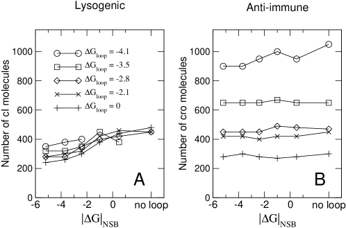
Figure 5: Steady-state total number of molecules of CI in the lysogenic state and of Cro in the anti-immune state, as a function of the DNA looping strength $\Delta G_{\textrm{loop}}$, for different values of the nonspecific binding strength $\Delta G_{\textrm{NSB}}$. The lysogenic CI concentration is in agreement with measured values and is rather insensitive to nonspecific binding, although DNA looping causes a decrease in the lysogenic CI concentration. The concentration of Cro in the anti-immune state is insensitive to DNA looping strength (as expected) but increases with the strength of the nonspecific binding interaction.

We note that although we have chosen $N$ as our order parameter, we could have made an alternative choice - for example, the total number of CI molecules, or some weighted combination of the numbers of CI and Cro. Providing these other choices give good separation of the initial and final states, the same rate constants and transition paths should be obtained. However, the computational efficiency and sampling effectiveness may be affected by the choice of order parameter.

The aim of the computation is to compute the rate $k$ at which the system makes transitions from the region where $N<N_{\textrm{lys}}$ to the region where $N>N_{\textrm{ai}}$. This is the frequency with which simulation trajectories leave the lysogenic state and enter the anti-immune state. This frequency is very low, but it can be re-expressed as TIS :

$$k=\Phi_{\textrm{lys}}P_{\textrm{lys}\to\textrm{ai}}$$ (7)

Here, $\Phi_{\textrm{lys}}$ is the flux of trajectories out of the lysogenic state, or the frequency with which the system crosses the interface $N=N_{\textrm{lys}}$ coming from the lysogenic state. This flux must be multiplied by the probability $P_{\textrm{lys}\to\textrm{ai}}$ that one of these trajectories which leaves the lysogenic state will subsequently reach the anti-immune state rather than returning to the lysogenic state. The flux $\Phi_{\textrm{lys}}$ can be calculated very accurately because the system makes many crossings of $N=N_{\textrm{lys}}$. The probability $P_{\textrm{lys}\to\textrm{ai}}$ is however very small and difficult to calculate. This problem can be overcome by placing a number of “interfaces” between the lysogenic and lytic states, at values of $N$ intermediate between $N_{\textrm{lys}}$ and $N_{\textrm{ai}}$. We define $N_{0}=N_{\textrm{lys}}$, $N_{n}=N_{\textrm{ai}}$, and place interfaces $N_{i}$ for $1\leq i\leq n-1$ between $N_{0}$ and $N_{n}$. Eq. (7) can then be rewritten as TIS :

$$k=\Phi_{\textrm{lys}}\prod_{i=0}^{n-1}P({N_{i+1}|N_{i}})$$ (8)

where $P({N_{i+1}|N_{i}})$ is the probability that a trajectory which has reached interface $N_{i}$, coming from the lysogenic state, will subsequently reach the next interface $N_{i+1}$, rather than returning to the lysogenic state. Since the interfaces may be placed arbitrarily close together, the probabilities $P({N_{i+1}|N_{i}})$ can be large, and thus easy to compute accurately. Once these probabilities and the flux $\Phi_{\textrm{lys}}$ have been computed, the rate for the lysogenic to anti-immune transition can be obtained using Eq.(8).

We compute the flux $\Phi_{\textrm{lys}}$ using a simulation run initiated in the lysogenic state. Every time the simulation crosses $N=N_{\textrm{lys}}$ in the direction of increasing $N$, we increment a counter. At the same time, we store the configuration of the system at the moment that the crossing occurs. At the end of this simulation run, we divide the value of our counter by the total simulation time to obtain $\Phi_{\textrm{lys}}$. We have also obtained a collection of system configurations corresponding to crossings of $N=N_{\textrm{lys}}$.

We now turn to the computation of the probabilities $P({N_{i+1}|N_{i}})$. To compute $P({N_{1}|N_{0}})$, we fire many “trial runs” from the collection of configurations that we have obtained at $N_{0}$. In each trial run, we choose a configuration at random from our collection and use it as the starting point for a new simulation run, which is continued until either the system reaches $N_{1}$, or it returns to the lysogenic state $N<N_{0}$. If $N_{1}$ is reached, the final configuration of the trial run is stored in a new collection. We repeat this trial run procedure many times, and finally estimate $P({N_{1}|N_{0}})$ as the fraction of trial runs that successfully reached $N_{1}$. We now use the collection of configurations which we have just collected at $N_{1}$ to compute $P({N_{2}|N_{1}})$: once again we fire many trial runs which are continued until either $N_{2}$ or $N_{0}$ is reached. We repeat this procedure for each interface, until we have computed all the $P({N_{i+1}|N_{i}})$ values. At this point, trajectories corresponding to transitions from the lysogenic to anti-immune states could be extracted by tracing back trial runs from $N_{\textrm{ai}}$ back to $N_{\textrm{lys}}$. An analysis of these trajectories could be used to investigate the transition mechanism. However, in this work we have confined ourselves to computing the rate constant $k$.

The frequency of transitions from the anti-immune to lysogenic states can be computed in the same way - here, our order parameter is simply taken to be

$$N^{\prime}={\mathrm{total~{}number~{}of~{}CI}}-{\mathrm{total~{}number~{}of~{}Cro}}$$ (9)

To obtain the results presented in this paper, we used 8-85 interfaces, with 1000-10000 configurations collected at $N_{0}$ and 500-10000 trial runs (precise values varied in each calculation). In addition, we averaged our results over 10-100 FFS calculations, to obtain an estimate for the error bars on our calculated rate constants. The final rate constants obtained are not dependent on the exact values of these parameters Allen06_1 ; Allen06_2. For implementations of FFS with very few ($\sim 10-50$) configurations at each interface, sampling errors may arise if the configurations most likely to progress to the final state are missed, especially if the order parameter poorly represents the progress of the transition sear ; bolhuis . These can be detected by the appearance of large variations between the rate constants calculated in different FFS runs. However, we have found this not to be the case when the chosen order parameter is reliable and the number of configurations is more than about 100, as in this work.

X Simulation Results

In this section, we present data on steady-state CI and Cro concentrations in the lysogenic and anti-immune states (X.1), depletion of free CI by nonspecific DNA binding, promoter activity as a function of lysogenic CI concentration (X.3), switch stability for the Little mutants, calculated using FSS (X.4) and the effects of increasing the RNAp concentration (X.5).

X.1 Steady-state protein concentrations

Figure 5 shows the average number of CI and Cro molecules in our simulations of the lysogenic and anti-immune states respectively, for different values of the parameters $\Delta G_{\textrm{loop}}$ and $\Delta G_{\textrm{NSB}}$. The model produces steady-state protein concentrations in agreement with measured values. The number of CI molecules in a wild-type lysogen has been measured to be 220 Reichardt71 , but is highly variable Baek03 . The concentration of Cro in the anti-immune state has been measured as $\sim 400\textrm{nM}$ Reinitz90 , so that in our assumed volume of 2$\textrm{$\mu$m}^{3}$ we expect $\sim 500$ molecules. Our model predicts that the steady-state CI level in the lysogen is rather stable to changes in the nonspecific DNA binding strength $\Delta G_{\textrm{NSB}}$. However, if the looping interaction is absent, the lysogenic state cannot be sustained when $\Delta G_{\textrm{NSB}}$ becomes large.

Increasing the strength of the DNA looping interaction decreases the lysogenic CI concentration by a factor of up to 2, in agreement with the observations of Dodd et al Dodd04 . In contrast, the level of Cro in the anti-immune state increases strongly with the strength of the nonspecific binding interaction, although it is insensitive to the DNA looping strength (as the DNA loop does not form in the anti-immune state). $P_{R}$ is repressed by Cro binding at $O_{R}1$ or $O_{R}2$. Depletion of free Cro by nonspecific binding reduces this autorepression, increasing expression of $P_{R}$, and increasing the total cellular Cro level.

X.2 Depletion of free transcription factors by nonspecific DNA binding

$\Delta G_{\textrm{NSB}}$ ( kcal/mol)	free monomers	free dimers	NSB dimers	percentage free CI
-2.1	76	75	37	75%
-2.8	52	48	76	49%
-3.5	23	24	115	24%
-4.1	18	9	132	12%

Table 2: Partioning of the intracellular CI pool into free monomers, free dimers and nonspecifically bound dimers, for several values of $\Delta G_{\textrm{NSB}}$, assuming a total of 300 CI molecules in the cell and ignoring specific DNA binding reactions. The percentage of the CI pool which is free [not DNA-bound] is shown in the right-hand column.

Table 2 shows the partioning of the total CI in the cell into free monomers, free dimers and nonspecifically bound dimers, assuming a total of 300 molecules in the cell and ignoring specific DNA binding. This demonstrates that the amount of free CI is dramatically depleted by nonspecific DNA binding, for the range of interaction strengths considered in this work.

X.3 Promoter Activity

In recent experiments by Dodd et al Dodd01 ; Dodd04 , the activity of the $P_{RM}$ and $P_{R}$ promoters was measured as a function of the intracellular CI concentration (supplied from a plasmid), for constructs with and without the DNA looping interaction Dodd01 ; Dodd04 . Fitting the resulting data with a thermodynamic binding model using in vitro measured binding constants showed that CI binding to $O_{R}$ was much weaker than expected Dodd01 ; Dodd04 . Similar effects are well-known for other promoters, including lac Hippel74 , and have been attributed to nonspecific binding of transcription factors to genomic DNA. Dodd et al Dodd01 ; Dodd04 and other authors Bakk04_1 ; Bakk04_2 fitted the measured promoter activity data with a model including nonspecific DNA binding. Although these promoter activity curves may be distorted due to plasmid copy number variation littledodd, the reduction in the apparent free CI concentration, apparently due to nonspecific binding, appears to be real and significant.

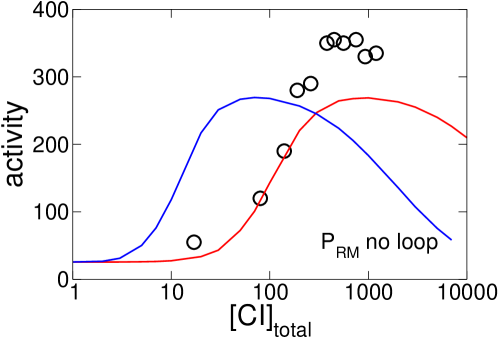
Figure 6: Computed activity of the $P_{RM}$ promoter, as a function of total cellular CI concentration. The red lines are computed with $\Delta G_{\textrm{NSB}}=-4.1\textrm{kcal/mol}$; the blue lines without nonspecific DNA binding. The symbols show the data of Dodd et al, 2001 (circles) and Dodd et al, 2004 (squares). (a): $P_{RM}$ activity in absence of DNA looping interaction.

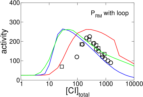
Figure 7: Computed activity of the $P_{RM}$ promoter, as a function of total cellular CI concentration. The red lines are computed with $\Delta G_{\textrm{NSB}}=-4.1\textrm{kcal/mol}$; the blue lines without nonspecific DNA binding. The symbols show the data of Dodd et al, 2001 (circles) and Dodd et al, 2004 (squares). $P_{RM}$ activity, with DNA looping. The red and blue lines are computed with $\Delta G_{\textrm{loop}}=-1\textrm{kcal/mol}$. The green line is computed with $\Delta G_{\textrm{loop}}=-3.7\textrm{kcal/mol}$ . The simulation data was multiplied by a scaling factor of 10000.

In Figures 6 and 7, we measure $P_{RM}$ activity as a function of fixed total CI concentration in our model (CI levels are fixed by turning off protein production; no Cro is present). Increasing the nonspecific binding strength (magnitude of $\Delta G_{\textrm{NSB}}$) shifts the promoter activity curves towards higher CI concentrations. The promoter activity data measured by Dodd et al, extracted from Refs Dodd01 and Dodd04 , are also shown in Figures 6 and 7. To convert Wild-type Lysogenic Units (WLU) to CI concentrations, we assumed a lysogenic CI concentration of 370nM Dodd04 . Without nonspecific DNA binding, our model completely fails to agree with the measured $P_{RM}$ activity curves (blue lines). By fitting their data to a model with strong nonspecific DNA binding [$\Delta G_{\textrm{NSB}}=-6.2\textrm{kcal/mol}$, with $6.76\times 10^{-3}\textrm{M}$ nonspecific binding site concentration], Dodd et al obtained a best-fit value of $-0.5\textrm{kcal/mol}$ for the DNA looping strength. In our model, the nonspecific binding is weaker compared to Dodd et al ($\Delta G_{\textrm{NSB}}\sim 2-4\textrm{kcal/mol}$; $1.0\times 10^{7}$ sites in a volume of $2\textrm{$\mu$m}$ - in the same volume, Dodd et al would have $1.35\times 10^{7}$ sites), and the DNA looping interaction is stronger. Dodd et al did not model the dynamics of the system, and therefore were not aiming to reproduce the stability of the lysogenic state. Our model, by contrast, is dynamical. We find that a strong looping interaction is needed to explain the stability and robustness of the lysogenic state; however, with our parameters, we do not fit the Dodd et al data well, as shown, for example, by the green line in Figure 7. Plasmid copy number variation may account for some of the discrepancy, as may our smaller value of $\Delta G_{\textrm{NSB}}$. However, the apparent discrepancy between the large value of $\Delta G_{\textrm{loop}}$ needed to obtain agreement with experimental observations in dynamical simulations, and the smaller value obtained from fitting promoter activity data, remains to be resolved.

X.4 Spontaneous switching times for the Little mutants

Mutant	$\Delta G_{\textrm{loop}}$	$\Delta G_{\textrm{NSB}}$	Switching time	Switching time
	kcal/mol	kcal/mol	lys. $\to$ anti-imm.	anti-imm. $\to$ lys.
			(generations)	(generations)
$O_{R}(121)$	-5.2	-4.1	$(1.1\pm 0.4)\times 10^{10}$	$9.5\pm 0.1$
$O_{R}(121)$	-3.7	-2.8	$(4\pm 3)\times 10^{15}$	$6.12\pm 0.02$
$O_{R}(121)$	-1.0	no NSB	lysogen monostable	anti-imm. unstable
$O_{R}(323)$	-5.2	-4.1	$450\pm 40$	$450\pm 30$
$O_{R}(323)$	-3.7	-2.8	$(3\pm 2)\times 10^{14}$	$190\pm 20$
$O_{R}(323)$	-1.0	no NSB	$130\pm 10$	$(2.5\pm 0.6)\times 10^{10}$

Table 3: Spontaneous switching times (inverse of calculated switching rates) for the Little mutants $O_{R}(121)$ and $O_{R}(323)$, computed as in Table 1 of the main text and assuming a cell generation time of 34 min.

We have used Forward Flux Sampling to compute spontaneous switching rates from the lysogenic to the anti-immune state, and vice versa, for the Little mutants $O_{R}(121)$ and $O_{R}(323)$. The computed rates were converted into typical numbers of cell generations for which we expect these states to be stable, using a generation time of 34 min. The results are shown in 3, for a range of values of the parameters $\Delta G_{\textrm{loop}}$ and $\Delta G_{\textrm{NSB}}$.

We note that in modeling these mutants, one must decide which pair of CI dimers bound at $O_{R}$ experiences a cooperative binding interaction. In our simulations, we assumed cooperative binding interactions for the first two adjacent CI dimers to bind.

X.5 Effects of RNA polymerase concentration

We tested the effect of the free RNA polymerase concentration, which was fixed at $50\textrm{nM}$ in our model. This value was obtained by McClure, by fitting in vivo promoter expression data mcclure1983_proc , but has recently been challenged Bremer2003 . We varied the free RNAp concentration and measured the total number of CI molecules in the lysogenic state. The results are plotted in Figure 8. Changing the free RNAp concentration can change the lysogenic CI concentration by about a factor of two. Although this parameter should be investigated further in future work, its value (within a reasonable physiological range) does not affect the qualitative features of our results. In fact, a higher free RNAp concentration is likely to further increase the stability of the lysogenic state.

Figure 8: Effect of changing the free RNA polymerase concentration. The total number of CI molecules in the lysogenic state is plotted as a function of the free RNAp concentration.

XI Sensitivity of our conclusions to parameter choice

Our computational model involves several hundred chemical reactions. Many of the rate constants for these reactions are identical, so that the number of parameters is significantly less than the number of reactions. Nevertheless, parameter choice remains an important issue. We have taken most of the parameters for our model from the extensive biochemical data on the phage $\lambda$ switch available in the literature, as discussed in the main text. However, these values are subject to uncertainty, and in a few cases were unavailable, forcing us to make educated guesses (as detailed in the main text). It is therefore appropriate to investigate how sensitive our conclusions are to the choice of parameters. It is clearly impossible for us to prove that our conclusions hold throughout the many-dimensional space of all possible parameter variations. Nevertheless, we can strengthen our conclusions by testing the effects of several parameter changes, selected with the biology of the system in mind. To this end, we chose two parameters which are particularly uncertain, and are especially likely to influence the switching rate. We repeated our simulations for different values of these parameters. These are (1) the number of free RNA polymerase molecules in the cell, and (2) the average number of Cro molecules produced per mRNA molecule (translational burst size). The free RNAp concentration has not been measured directly in experiments, and inferred values are subject to a large range of uncertainty. The translational burst size is also rather uncertain from biochemical data. The burst size for Cro is likely to be particularly important because is possible that a burst of Cro molecules produced from a single mRNA might be sufficient to flip the switch. We varied the burst size by increasing the translation rate while proportionately decreasing the transcription rate, so as to keep the average Cro level in the cell approximately constant. Figures 9 and 10 show the range of bistability for the model switch, as a function of the nonspecific DNA binding and DNA looping strengths, for free RNAp concentration doubled compared to the “standard” model [100nM instead of 50nM] 9 and Cro translational burst size doubled [40 per transcript instead of 20] 10. Both these plots show the same qualitative behaviour as we obtained for the “standard” parameter set, as shown in Fig. 3 of the main text. As the DNA looping strength increases, the range of nonspecific binding strengths over which the switch is bistable increases. We also used Forward Flux Sampling to compute switching rates for the lysogenic to anti-immune transition, in the case where the translational burst size for Cro was doubled. The results are shown in Table 4.

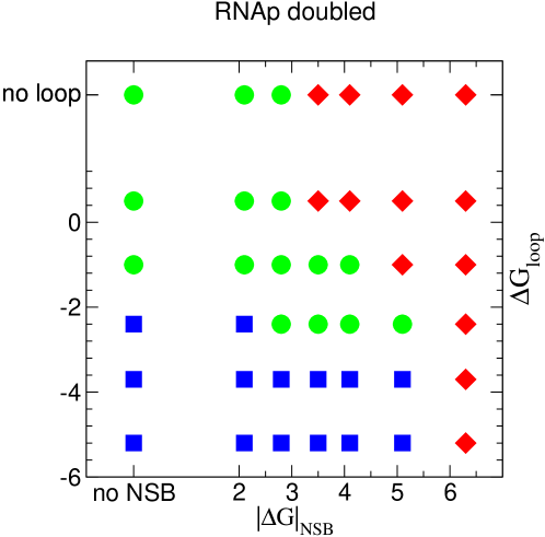
Figure 9: Range of bistability of the model switch as a function of the nonspecific DNA binding and DNA looping strengths, for a parameter set where the free RNAp concentration has been doubled [100nM instead of 50nM]. Comparing these results to those of Fig. 3 in the main text shows that our main conclusion, namely that DNA looping stabilises the switch against nonspecific DNA binding, also holds for these modified parameter sets.

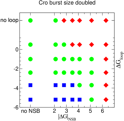
Figure 10: Range of bistability of the model switch as a function of the nonspecific DNA binding and DNA looping strengths, for a parameter set where the average number of Cro molecules produced per mRNA transcript has been doubled [40 instead of 20] by doubling the translation rate while halving the transcription rate. Comparing these results to those of Fig. 3 in the main text shows that our main conclusion, namely that DNA looping stabilises the switch against nonspecific DNA binding, also holds for these modified parameter sets.

$\Delta G_{\textrm{loop}}$	$\Delta G_{\textrm{NSB}}$	Switching time
kcal/mol	kcal/mol	lys. $\to$ anti-imm.
		(generations)
no loop	no NSB	$(1.5\pm 0.2)\times 10^{7}$
no loop	-2.1	$(2.3\pm 0.1)\times 10^{5}$
-2.4	no NSB	$(1.5\pm 0.4)\times 10^{11}$
-2.4	-2.1	$(2.7\pm 0.2)\times 10^{13}$

Table 4: Spontaneous switching times (inverse of calculated switching rates) for the model switch with Cro translational burst size doubled, by doubling the translation rate while halving the transcription rate.

Our main conclusions, that the lysogen is destabilized by nonspecific DNA binding but stabilized by the DNA looping interaction, remain the same with this modified parameter set. Comparing the two results without DNA looping in Table 4, the switching time in the presence of nonspecific DNA binding is two orders of magnitude faster than when nonspecific binding is absent. Comparing the results with and without DNA looping, we find that the looping interaction stabilises the lysogen by a factor of $10^{4}$ in the absence of nonspecific binding and by a factor of $10^{6}$ when nonspecific binding is present. These switching rates, together with the bistability analysis of Figs. 9 and 10, suggest that the conclusions arising from this work are likely to be robust to uncertainties in the parameter values.

XII Components and Reactions

XII.1 List of Components

This is the list of components for our basic model, without non-specific binding and without looping. With the notation O(XYZ) we refer to the operator O_R where X is bound to the site O_R3, Y is bound to O_R2 and Z is bound to O_R1. $\{{\rm X,Y,Z}\}=\{{\rm 0,R,C,R_{p}}\}$, where 0 corresponds to an empty site, R corresponds to CI dimer bound, C to a Cro dimer bound, and ${\rm R_{p}}$ to an RNA polymerase molecule bound. The Cro promoter, $P_{R}$ overlaps with O_R3, whereas the CI promoter, $P_{RM}$ overlaps with both O_R2 and O_R1, in our notation, RNA polymerase binds either to the X slot or to Y and Z simultaneously.

1 CI
2 Cro
3 CI₂
4 Cro₂
5 Rp
6 O(000)
7 O(R00)
8 O(0R0)
9 O(00R)
10 O(C00)
11 O(0C0)
12 O(00C)
13 O(Rp00)
14 O(0Rp)
15 O(RR0)
16 O(ROR)
17 O(RC0)
18 O(R0C)
19 O(RRp)
20 O(0RR)
21 O(CR0)
22 O(0RC)
23 O(RpR0
24 O(C0R)
25 O(OCR)
26 O(Rp0R)
27 O(CC0)
28 O(C0C)
29 O(CRp)
30 O(0CC)
31 O(RpC0)
32 O(Rp0C)
33 O(RRR)
34 O(RRC)
35 O(RCR)
36 O(CRR)
37 O(RpRR)
38 O(RCC)
39 O(CRC)
40 O(CCR)
41 O(RpCR)
42 O(RpRC)
43 O(CCC)
44 O(RpCC)
45 O(RpRp)
46 MCI
47 MCro
Adding nonspecific DNA binding requires 3 extra species:
48 D
49 DCI₂
50 DCro₂
When DNA looping is to be included in the model, we consider also the left operator O_L, which also has three binding sites for transcription factors. RNA polymerase can bind to promoter $P_{L}$, which overlaps with the binding site O_L1. The two operator can interact via a DNA loop stabilised by the octamerization of two CI tetramers which are already bound on adjacent sites on the two operators. We label these looped states according to which pairs of CI dimers form the octamer. Looped states obtained by interaction between CI tetramers bound to O_R1, O_R2,O_L1 and O_L2 are denoted OLR1. States OLR2 have loops formed by interactions between tetramers bound to O_R1, O_R2, O_L2 and O_L3. States denoted OLR3 have loops formed by interaction between tetramers bound to O_R2, O_R3, O_L1 and O_L2. Finally, states denoted OLR4 have loops formed by interaction between tetramers bound to O_R2, O_R3, O_L2 and O_L3. Each of these loop categories has two additional sites to which transcription factor dimers can bind. We therefore denote a particular looped configuration by OLRX(YZ), where X refers to loop type 1-4 (as above), Y denotes which species occupies the non-octamerized site on O_L and Z labels the occupation of the non-octamerized site on O_R. The extra species required in the model with looping are:
51 OL(000)
52 OL(R00)
53 OL(0R0)
54 OL(00R)
55 OL(C00)
56 OL(0C0)
57 OL(00C)
58 OL(00Rp)
59 OL(RR0)
60 OL(R0R)
61 OL(RCO)
62 OL(R0C)
63 OL(R0Rp)
64 OL(0RR)
65 OL(CR0)
66 OL(0RC)
67 OL(0RRp)
68 OL(C0R)
69 OL(0CR)
70 OL(CC0)
71 OL(C0C)
72 OL(C0Rp)
73 OL(0CC)
74 OL(0CRp)
75 OL(RRR)
76 OL(RRC)
77 OL(RRRp)
78 OL(RCR)
79 OL(CRR)
80 OL(RCC)
81 OL(RCRp)
82 OL(CRC)
83 OL(CRRp)
84 OL(CCR)
85 OL(CCC)
86 OL(CCRp)
87 OLR1(00)
88 OLR1(0R)
89 OLR1(0C)
90 OLR1(0Rp)
91 OLR1(R0)
92 OLR1(RR)
93 OLR1(RC)
94 OLR1(RRp)
95 OLR1(C0)
96 OLR1(CR)
97 OLR1(CC)
98 OLR1(CRp)
99 OLR2(00)
100 OLR2(0R)
101 OLR2(0C)
102 OLR2(0Rp)
103 OLR2(R0)
104 OLR2(RR)
105 OLR2(RC)
106 OLR2(RRp)
107 OLR2(C0)
108 OLR2(CR)
109 OLR2(CC)
110 OLR2(CRp)
111 OLR3(00)
112 OLR3(0R)
113 OLR3(0C)
114 OLR3(R0)
115 OLR3(RR)
116 OLR3(RC)
117 OLR3(C0)
118 OLR3(CR)
119 OLR3(CC)
120 OLR4(00)
121 OLR4(0R)
122 OLR4(0C)
123 OLR4(R0)
124 OLR4(RR)
125 OLR4(RC)
126 OLR4(C0)
127 OLR4(CR)
128 OLR4(CC)
129 OLR2(Rp0)
130 OLR2(RpR)
131 OLR2(RpC)
132 OLR2(RpRp)
133 OLR4(Rp0)
134 OLR4(RpR)
135 OLR4(RpC)

XII.2 List of reactions

This set is obtained with $\Delta G_{\rm loop}=-5.2$ kcal/mol and $\Delta G_{\rm NSB}=-3.5$ kcal/mol.
1) CI + CI $\to$ CI₂ k = 0.628319
2) CI₂ $\to$ CI + CI k = 5.705413
3) Cro + Cro $\to$ Cro₂ k = 0.628319
4) Cro₂ $\to$ Cro + Cro k = 280.199086
5) O(000) + CI₂ $\to$ O(R00) k = 0.314159
6) O(R00 $\to$ O(000) + CI₂ k = 38.256936
7) O(000) + CI₂ $\to$ O(0R0) k = 0.314159
8) O(0R0) $\to$ O(000) + CI₂ k = 7.551827
9) O(000) + CI₂ $\to$ O(00R) k = 0.314159
10) O(00R) $\to$ O(000) + CI₂ k = 0.294263
11) O(000) + Cro₂ $\to$ O(C00) k = 0.314159
12) O(C00) $\to$ O(000) + Cro₂ k = 0.068319
13) O(000) + Cro₂ $\to$ O(0C0) k = 0.314159
14) O(0C0) $\to$ O(000) + Cro₂ k = 4.641460
15) O(000) + Cro₂ $\to$ O(00C) k = 0.314159
16) O(00C) $\to$ O(000) + Cro₂ k = 0.662315
17) O(000) + Rp $\to$ O(Rp00) k = 0.314159
18) O(Rp00) $\to$ O(000) + Rp k = 1.490712
19) O(000) + Rp $\to$ O(0Rp) k = 0.314159
20) O(0Rp) $\to$ O(000) + Rp k = 0.294263
21) O(R00) + CI₂ $\to$ O(RR0) k = 0.314159
22) O(RR0) $\to$ O(R00) + CI₂ k = 0.068319
23) O(R00) + CI₂ $\to$ O(ROR) k = 0.314159
24) O(ROR) $\to$ O(R00) + CI₂ k = 0.294263
25) O(R00) + Cro₂ $\to$ O(RC0) k = 0.314159
26) O(RC0) $\to$ O(R00) + Cro₂ k = 4.641460
27) O(R00) + Cro₂ $\to$ O(R0C) k = 0.314159
28) O(R0C) $\to$ O(R00) + Cro₂ k = 0.662315
29) O(R00) + Rp $\to$ O(RRp) k = 0.314159
30) O(RRp) $\to$ O(R00) + Rp k = 0.294263
31) O(0R0) + CI₂ $\to$ O(RR0) k = 0.314159
32) O(RR0) $\to$ O(0R0) + CI₂ k = 0.346100
33) O(0R0) + CI₂ $\to$ O(0RR) k = 0.314159
34) O(0RR) $\to$ O(0R0) + CI₂ k = 0.003683
35) O(0R0) + Cro₂ $\to$ O(CR0) k = 0.314159
36) O(CR0) $\to$ O(0R0) + Cro₂ k = 0.068319
37) O(0R0) + Cro₂ $\to$ O(0RC) k = 0.314159
38) O(0RC) $\to$ O(0R0) + Cro₂ k = 0.662315
39) O(0R0) + Rp $\to$ O(RpR0) k = 0.314159
40) O(RpR0) $\to$ O(0R0) + Rp k = 1.490712
41) O(00R) + CI₂ $\to$ O(ROR) k = 0.314159
42) O(ROR) $\to$ O(00R) + CI₂ k = 38.256936
43) O(00R) + CI₂ $\to$ O(0RR) k = 0.314159
44) O(0RR) $\to$ O(00R) + CI₂ k = 0.094509
45) O(00R) + Cro₂ $\to$ O(C0R) k = 0.314159
46) O(C0R) $\to$ O(00R) + Cro₂ k = 0.068319
47) O(00R) + Cro₂ $\to$ O(0CR) k = 0.314159
48) O(0CR) $\to$ O(00R) + Cro₂ k = 4.641460
49) O(00R) + Rp $\to$ O(Rp0R) k = 0.314159
50) O(Rp0R) $\to$ O(00R) + Rp k = 1.490712
51) O(C00) + CI₂ $\to$ O(CR0) k = 0.314159
52) O(CR0) $\to$ O(C00) + CI₂ k = 7.551827
53) O(C00) + CI₂ $\to$ O(C0R) k = 0.314159
54) O(C0R) $\to$ O(C00) + CI₂ k = 0.294263
55) O(C00) + Cro₂ $\to$ O(CC0) k = 0.314159
56) O(CC0) $\to$ O(C00) + Cro₂ k = 1.753314
57) O(C00) + Cro₂ $\to$ O(C0C) k = 0.314159
58) O(C0C) $\to$ O(C00) + Cro₂ k = 0.662315
59) O(C00) + Rp $\to$ O(CRp) k = 0.314159
60) O(CRp) $\to$ O(C00) + Rp k = 0.294263
61) O(0C0) + CI₂ $\to$ O(RC0) k = 0.314159
62) O(RC0) $\to$ O(0C0) + CI₂ k = 38.256936
63) O(0C0) + CI₂ $\to$ O(0CR) k = 0.314159
64) O(0CR) $\to$ O(0C0) + CI₂ k = 0.294263
65) O(0C0) + Cro₂ $\to$ O(CC0) k = 0.314159
66) O(CC0) $\to$ O(0C0) + Cro₂ k = 0.025808
67) O(0C0) + Cro₂ $\to$ O(0CC) k = 0.314159
68) O(0CC) $\to$ O(0C0) + Cro₂ k = 0.130739
69) O(0C0) + Rp $\to$ O(RpC0) k = 0.314159
70) O(RpC0) $\to$ O(0C0) + Rp k = 1.490712
71) O(00C) + CI₂ $\to$ O(R0C) k = 0.314159
72) O(R0C) $\to$ O(00C) + CI₂ k = 38.256936
73) O(00C) + CI₂ $\to$ O(0RC) k = 0.314159
74) O(0RC) $\to$ O(00C) + CI₂ k = 7.551827
75) O(00C) + Cro₂ $\to$ O(C0C) k = 0.314159
76) O(C0C) $\to$ O(00C) + Cro₂ k = 0.068319
77) O(00C) + Cro₂ $\to$ O(0CC) k = 0.314159
78) O(0CC) $\to$ O(00C) + Cro₂ k = 0.916213
79) O(00C) + Rp $\to$ O(Rp0C) k = 0.314159
80) O(Rp0C) $\to$ O(00C) + Rp k = 1.490712
81) O(Rp00) + CI₂ $\to$ O(RpR0) k = 0.314159
82) O(RpR0) $\to$ O(Rp00) + CI₂ k = 7.551827
83) O(Rp00) + CI₂ $\to$ O(Rp0R) k = 0.314159
84) O(Rp0R) $\to$ O(Rp00) + CI₂ k = 0.294263
85) O(Rp00) + Cro₂ $\to$ O(RpC0) k = 0.314159
86) O(RpC0) $\to$ O(Rp00) + Cro₂ k = 4.641460
87) O(Rp00) + Cro₂ $\to$ O(Rp0C) k = 0.314159
88) O(Rp0C) $\to$ O(Rp00) + Cro₂ k = 0.662315
89) O(Rp00) + Rp $\to$ O(RpRp) k = 0.314159
90) O(RpRp) $\to$ O(Rp00) + Rp k = 0.294263
91) O(0Rp) + CI₂ $\to$ O(RRp) k = 0.314159
92) O(RRp) $\to$ O(0Rp) + CI₂ k = 38.256936
93) O(0Rp) + Cro₂ $\to$ O(CRp) k = 0.314159
94) O(CRp) $\to$ O(0Rp) + Cro₂ k = 0.068319
95) O(0Rp) + Rp $\to$ O(RpRp) k = 0.314159
96) O(RpRp) $\to$ O(0Rp) + Rp k = 1.490712
97) O(RR0) + CI₂ $\to$ O(RRR) k = 0.314159
98) O(RRR) $\to$ O(RR0) + CI₂ k = 0.407068
99) O(RR0) + Cro₂ $\to$ O(RRC) k = 0.314159
100) O(RRC) $\to$ O(RR0) + Cro₂ k = 0.662315
101) O(ROR) + CI₂ $\to$ O(RRR) k = 0.314159
102) O(RRR) $\to$ O(ROR) + CI₂ k = 0.094509
103) O(ROR) + Cro₂ $\to$ O(RCR) k = 0.314159
104) O(RCR) $\to$ O(ROR) + Cro₂ k = 4.641460
105) O(0RR) + CI₂ $\to$ O(RRR) k = 0.314159
106) O(RRR) $\to$ O(0RR) + CI₂ k = 38.256936
107) O(0RR) + Cro₂ $\to$ O(CRR) k = 0.314159
108) O(CRR) $\to$ O(0RR) + Cro₂ k = 0.068319
109) O(0RR) + Rp $\to$ O(RpRR) k = 0.314159
110) O(RpRR) $\to$ O(0RR) + Rp k = 1.490712
111) O(RC0) + CI₂ $\to$ O(RCR) k = 0.314159
112) O(RCR) $\to$ O(RC0) + CI₂ k = 0.294263
113) O(RC0) + Cro₂ $\to$ O(RCC) k = 0.314159
114) O(RCC) $\to$ O(RC0) + Cro₂ k = 0.130739
115) O(R0C) + CI₂ $\to$ O(RRC) k = 0.314159
116) O(RRC) $\to$ O(R0C) + CI₂ k = 0.068319
117) O(R0C) + Cro₂ $\to$ O(RCC) k = 0.314159
118) O(RCC) $\to$ O(R0C) + Cro₂ k = 1.753314
119) O(CR0) + CI₂ $\to$ O(CRR) k = 0.314159
120) O(CRR) $\to$ O(CR0) + CI₂ k = 0.003683
121) O(CR0) + Cro₂ $\to$ O(CRC) k = 0.314159
122) O(CRC) $\to$ O(CR0) + Cro₂ k = 0.662315
123) O(C0R) + CI₂ $\to$ O(CRR) k = 0.314159
124) O(CRR) $\to$ O(C0R) + CI₂ k = 0.094509
125) O(C0R) + Cro₂ $\to$ O(CCR) k = 0.314159
126) O(CCR) $\to$ O(C0R) + Cro₂ k = 1.753314
127) O(0CR) + CI₂ $\to$ O(RCR) k = 0.314159
128) O(RCR) $\to$ O(0CR) + CI₂ k = 38.256936
129) O(0CR) + Cro₂ $\to$ O(CCR) k = 0.314159
130) O(CCR) $\to$ O(0CR) + Cro₂ k = 0.025808
131) O(0CR) + Rp $\to$ O(RpCR) k = 0.314159
132) O(RpCR) $\to$ O(0CR) + Rp k = 1.490712
133) O(0RC) + CI₂ $\to$ O(RRC) k = 0.314159
134) O(RRC) $\to$ O(0RC) + CI₂ k = 0.346100
135) O(0RC) + Cro₂ $\to$ O(CRC) k = 0.314159
136) O(CRC) $\to$ O(0RC) + Cro₂ k = 0.068319
137) O(0RC) + Rp $\to$ O(RpRC) k = 0.314159
138) O(RpRC) $\to$ O(0RC) + Rp k = 1.490712
139) O(CC0) + CI₂ $\to$ O(CCR) k = 0.314159
140) O(CCR) $\to$ O(CC0) + CI₂ k = 0.294263
141) O(CC0) + Cro₂ $\to$ O(CCC) k = 0.314159
142) O(CCC) $\to$ O(CC0) + Cro₂ k = 0.407068
143) O(C0C) + CI₂ $\to$ O(CRC) k = 0.314159
144) O(CRC) $\to$ O(C0C) + CI₂ k = 7.551827
145) O(C0C) + Cro₂ $\to$ O(CCC) k = 0.314159
146) O(CCC) $\to$ O(C0C) + Cro₂ k = 1.077612
147) O(0CC) + CI₂ $\to$ O(RCC) k = 0.314159
148) O(RCC) $\to$ O(0CC) + CI₂ k = 38.256936
149) O(0CC) + Cro₂ $\to$ O(CCC) k = 0.314159
150) O(CCC) $\to$ O(0CC) + Cro₂ k = 0.080354
151) O(0CC) + Rp $\to$ O(RpCC) k = 0.314159
152) O(RpCC) $\to$ O(0CC) + Rp k = 1.490712
153) O(RpR0) + CI₂ $\to$ O(RpRR) k = 0.314159
154) O(RpRR) $\to$ O(RpR0) + CI₂ k = 0.003683
155) O(RpR0) + Cro₂ $\to$ O(RpRC) k = 0.314159
156) O(RpRC) $\to$ O(RpR0) + Cro₂ k = 0.662315
157) O(Rp0R) + CI₂ $\to$ O(RpRR) k = 0.314159
158) O(RpRR) $\to$ O(Rp0R) + CI₂ k = 0.094509
159) O(Rp0R) + Cro₂ $\to$ O(RpCR) k = 0.314159
160) O(RpCR) $\to$ O(Rp0R) + Cro₂ k = 4.641460
161) O(RpC0) + CI₂ $\to$ O(RpCR) k = 0.314159
162) O(RpCR) $\to$ O(RpC0) + CI₂ k = 0.294263
163) O(RpC0) + Cro₂ $\to$ O(RpCC) k = 0.314159
164) O(RpCC) $\to$ O(RpC0) + Cro₂ k = 0.130739
165) O(Rp0C) + CI₂ $\to$ O(RpRC) k = 0.314159
166) O(RpRC) $\to$ O(Rp0C) + CI₂ k = 7.551827
167) O(Rp0C) + Cro₂ $\to$ O(RpCC) k = 0.314159
168) O(RpCC) $\to$ O(Rp0C) + Cro₂ k = 1.753314
169) O(Rp00) $\to$ O(000) + Rp + MCI k = 0.001000
170) O(RpR0) $\to$ O(0R0) + Rp + MCI k = 0.011000
171) O(Rp0R) $\to$ O(00R) + Rp + MCI k = 0.001000
172) O(RpC0) $\to$ O(0C0) + Rp + MCI k = 0.001000
173) O(Rp0C) $\to$ O(00C) + Rp + MCI k = 0.001000
174) O(RpRR) $\to$ O(0RR) + Rp + MCI k = 0.011000
175) O(RpRC) $\to$ O(0RC) + Rp + MCI k = 0.011000
176) O(RpCR) $\to$ O(0CR) + Rp + MCI k = 0.001000
177) O(RpCC) $\to$ O(0CC) + Rp + MCI k = 0.001000
178) O(RpRp) $\to$ O(0Rp) + Rp + MCI k = 0.001000
179) O(0Rp) $\to$ O(000)+ Rp + MCro k = 0.014000
180) O(RRp) $\to$ O(R00) + Rp + MCro k = 0.014000
181) O(CRp) $\to$ O(C00) + Rp + MCro k = 0.014000
182) O(RpRp) $\to$ O(Rp00) + Rp + MCro k = 0.014000
183) MCI $\to$ MCI + CI k = 0.034656
184) MCro $\to$ MCro + Cro k = 0.115520
185) MCI $\to$ 0 k = 0.005776
186) MCro $\to$ 0 k = 0.005776
187) CI $\to$ 0 k = 0.000340
188) Cro $\to$ 0 k = 0.000606
189) CI₂ $\to$ 0 k = 0.000340
190) Cro₂ $\to$ 0 k = 0.000340

If the system includes looping, the reaction schemes should be extended with the following reactions (rate constants calculated for $\Delta G_{\rm loop}=-5.2$ kcal/mol):

191) OL(000) + CI₂ $\to$ OL(R00) k = 0.314159
192) OL(R00) $\to$ OL(000) + CI₂ k = 0.346100
193) OL(000) + CI₂ $\to$ OL(0R0) k = 0.314159
194) OL(0R0) $\to$ OL(000) + CI₂ k = 0.563117
195) OL(000) + CI₂ $\to$ OL(00R) k = 0.314159
196) OL(00R) $\to$ OL(000) + CI₂ k = 0.035701
197) OL(000) + Cro₂ $\to$ OL(C00) k = 0.314159
198) OL(C00) $\to$ OL(000) + Cro₂ k = 0.068319
199) OL(000) + Cro₂ $\to$ OL(0C0) k = 0.314159
200) OL(0C0) $\to$ OL(000) + Cro₂ k = 4.641460
201) OL(000) + Cro₂ $\to$ OL(00C) k = 0.314159
202) OL(00C) $\to$ OL(000) + Cro₂ k = 0.662315
203) OL(000) + Rp $\to$ OL(00Rp) k = 0.314159
204) OL(00Rp) $\to$ OL(000) + Rp k = 2.062175
205) OL(R00) + CI₂ $\to$ OL(RR0) k = 0.314159
206) OL(RR0) $\to$ OL(R00) + CI₂ k = 0.009749
207) OL(R00) + CI₂ $\to$ OL(R0R) k = 0.314159
208) OL(R0R) $\to$ OL(R00) + CI₂ k = 0.035701
209) OL(R00) + Cro₂ $\to$ OL(RCO) k = 0.314159
210) OL(RCO) $\to$ OL(R00) + Cro₂ k = 4.641460
211) OL(R00) + Cro₂ $\to$ OL(R0C) k = 0.314159
212) OL(R0C) $\to$ OL(R00) + Cro₂ k = 0.662315
213) OL(R00) + Rp $\to$ OL(R0Rp) k = 0.314159
214) OL(R0Rp) $\to$ OL(R00) + Rp k = 2.062175
215) OL(0R0) + CI₂ $\to$ OL(RR0 k = 0.314159
216) OL(RR0) $\to$ OL(0R0) + CI₂ k = 0.005992
217) OL(0R0) + CI₂ $\to$ OL(0RR) k = 0.314159
218) OL(0RR) $\to$ OL(0R0) + CI₂ k = 0.000618
219) OL(0R0) + Cro₂ $\to$ OL(CR0) k = 0.314159
220) OL(CR0) $\to$ OL(0R0) + Cro₂ k = 0.068319
221) OL(0R0) + Cro₂ $\to$ OL(0RC) k = 0.314159
222) OL(0RC) $\to$ OL(0R0) + Cro₂ k = 0.662315
223) OL(0R0) + Rp $\to$ OL(0RRp) k = 0.314159
224) OL(0RRp) $\to$ OL(0R0) + Rp k = 2.062175
225) OL(00R) + CI₂ $\to$ OL(R0R) k = 0.314159
226) OL(R0R) $\to$ OL(00R) + CI₂ k = 0.346100
227) OL(00R) + CI₂ $\to$ OL(0RR) k = 0.314159
228) OL(0RR) $\to$ OL(00R) + CI₂ k = 0.009749
229) OL(00R) + Cro₂ $\to$ OL(C0R) k = 0.314159
230) OL(C0R) $\to$ OL(00R) + Cro₂ k = 0.068319
231) OL(00R) + Cro₂ $\to$ OL(0CR) k = 0.314159
232) OL(0CR) $\to$ OL(00R) + Cro₂ k = 4.641460
233) OL(C00) + CI₂ $\to$ OL(CR0) k = 0.314159
234) OL(CR0) $\to$ OL(C00) + CI₂ k = 0.563117
235) OL(C00) + CI₂ $\to$ OL(C0R) k = 0.314159
236) OL(C0R) $\to$ OL(C00) + CI₂ k = 0.035701
237) OL(C00) + Cro₂ $\to$ OL(CC0) k = 0.314159
238) OL(CC0) $\to$ OL(C00) + Cro₂ k = 1.753314
239) OL(C00) + Cro₂ $\to$ OL(C0C) k = 0.314159
240) OL(C0C) $\to$ OL(C00) + Cro₂ k = 0.662315
241) OL(C00) + Rp $\to$ OL(C0Rp) k = 0.314159
242) OL(C0Rp) $\to$ OL(C00) + Rp k = 2.062175
243) OL(0C0) + CI₂ $\to$ OL(RCO) k = 0.314159
244) OL(RCO) $\to$ OL(0C0) + CI₂ k = 0.346100
245) OL(0C0) + CI₂ $\to$ OL(0CR) k = 0.314159
246) OL(0CR) $\to$ OL(0C0) + CI₂ k = 0.035701
247) OL(0C0) + Cro₂ $\to$ OL(CC0) k = 0.314159
248) OL(CC0) $\to$ OL(0C0) + Cro₂ k = 0.025808
249) OL(0C0) + Cro₂ $\to$ OL(0CC) k = 0.314159
250) OL(0CC) $\to$ OL(0C0) + Cro₂ k = 0.130739
251) OL(0C0) + Rp $\to$ OL(0CRp) k = 0.314159
252) OL(0CRp) $\to$ OL(0C0) + Rp k = 2.062175
253) OL(00C) + CI₂ $\to$ OL(R0C) k = 0.314159
254) OL(R0C) $\to$ OL(00C) + CI₂ k = 0.346100
255) OL(00C) + CI₂ $\to$ OL(0RC) k = 0.314159
256) OL(0RC) $\to$ OL(00C) + CI₂ k = 0.563117
257) OL(00C) + Cro₂ $\to$ OL(C0C) k = 0.314159
258) OL(C0C) $\to$ OL(00C) + Cro₂ k = 0.068319
259) OL(00C) + Cro₂ $\to$ OL(0CC) k = 0.314159
260) OL(0CC) $\to$ OL(00C) + Cro₂ k = 0.916213
261) OL(00Rp) + CI₂ $\to$ OL(R0Rp) k = 0.314159
262) OL(R0Rp) $\to$ OL(00Rp) + CI₂ k = 0.346100
263) OL(00Rp) + CI₂ $\to$ OL(0RRp) k = 0.314159
264) OL(0RRp) $\to$ OL(00Rp) + CI₂ k = 0.563117
265) OL(00Rp) + Cro₂ $\to$ OL(C0Rp) k = 0.314159
266) OL(C0Rp) $\to$ OL(00Rp) + Cro₂ k = 0.068319
267) OL(00Rp) + Cro₂ $\to$ OL(0CRp) k = 0.314159
268) OL(0CRp) $\to$ OL(00Rp) + Cro₂ k = 4.641460
269) OL(RR0) + CI₂ $\to$ OL(RRR) k = 0.314159
270) OL(RRR) $\to$ OL(RR0) + CI₂ k = 0.035701
271) OL(RR0) + Cro₂ $\to$ OL(RRC) k = 0.314159
272) OL(RRC) $\to$ OL(RR0) + Cro₂ k = 0.662315
273) OL(RR0) + Rp $\to$ OL(RRRp) k = 0.314159
274) OL(RRRp) $\to$ OL(RR0) + Rp k = 2.062175
275) OL(R0R) + CI₂ $\to$ OL(RRR) k = 0.314159
276) OL(RRR) $\to$ OL(R0R) + CI₂ k = 0.009749
277) OL(R0R) + Cro₂ $\to$ OL(RCR) k = 0.314159
278) OL(RCR) $\to$ OL(R0R) + Cro₂ k = 4.641460
279) OL(0RR) + CI₂ $\to$ OL(RRR) k = 0.314159
280) OL(RRR) $\to$ OL(0RR) + CI₂ k = 0.346100
281) OL(0RR) + Cro₂ $\to$ OL(CRR) k = 0.314159
282) OL(CRR) $\to$ OL(0RR) + Cro₂ k = 0.068319
283) OL(RCO) + CI₂ $\to$ OL(RCR) k = 0.314159
284) OL(RCR) $\to$ OL(RCO) + CI₂ k = 0.035701
285) OL(RCO) + Cro₂ $\to$ OL(RCC) k = 0.314159
286) OL(RCC) $\to$ OL(RCO) + Cro₂ k = 0.130739
287) OL(RCO) + Rp $\to$ OL(RCRp) k = 0.314159
288) OL(RCRp) $\to$ OL(RCO) + Rp k = 2.062175
289) OL(R0C) + CI₂ $\to$ OL(RRC) k = 0.314159
290) OL(RRC) $\to$ OL(R0C) + CI₂ k = 0.009749
291) OL(R0C) + Cro₂ $\to$ OL(RCC) k = 0.314159
292) OL(RCC) $\to$ OL(R0C) + Cro₂ k = 1.753314
293) OL(CR0) + CI₂ $\to$ OL(CRR) k = 0.314159
294) OL(CRR) $\to$ OL(CR0) + CI₂ k = 0.000618
295) OL(CR0) + Cro₂ $\to$ OL(CRC) k = 0.314159
296) OL(CRC) $\to$ OL(CR0) + Cro₂ k = 0.662315
297) OL(CR0) + Rp $\to$ OL(CRRp) k = 0.314159
298) OL(CRRp) $\to$ OL(CR0) + Rp k = 2.062175
299) OL(C0R) + CI₂ $\to$ OL(CRR) k = 0.314159
300) OL(CRR) $\to$ OL(C0R) + CI₂ k = 0.009749
301) OL(C0R) + Cro₂ $\to$ OL(CCR) k = 0.314159
302) OL(CCR) $\to$ OL(C0R) + Cro₂ k = 1.753314
303) OL(0CR) + CI₂ $\to$ OL(RCR) k = 0.314159
304) OL(RCR) $\to$ OL(0CR) + CI₂ k = 0.346100
305) OL(0CR) + Cro₂ $\to$ OL(CCR) k = 0.314159
306) OL(CCR) $\to$ OL(0CR) + Cro₂ k = 0.025808
307) OL(0RC) + CI₂ $\to$ OL(RRC) k = 0.314159
308) OL(RRC) $\to$ OL(0RC) + CI₂ k = 0.005992
309) OL(0RC) + Cro₂ $\to$ OL(CRC) k = 0.314159
310) OL(CRC) $\to$ OL(0RC) + Cro₂ k = 0.068319
311) OL(CC0) + CI₂ $\to$ OL(CCR) k = 0.314159
312) OL(CCR) $\to$ OL(CC0) + CI₂ k = 0.035701
313) OL(CC0) + Cro₂ $\to$ OL(CCC) k = 0.314159
314) OL(CCC) $\to$ OL(CC0) + Cro₂ k = 0.407068
315) OL(CC0) + Rp $\to$ OL(CCRp) k = 0.314159
316) OL(CCRp) $\to$ OL(CC0) + Rp k = 2.062175
317) OL(C0C) + CI₂ $\to$ OL(CRC) k = 0.314159
318) OL(CRC) $\to$ OL(C0C) + CI₂ k = 0.563117
319) OL(C0C) + Cro₂ $\to$ OL(CCC) k = 0.314159
320) OL(CCC) $\to$ OL(C0C) + Cro₂ k = 1.077612
321) OL(0CC) + CI₂ $\to$ OL(RCC) k = 0.314159
322) OL(RCC) $\to$ OL(0CC) + CI₂ k = 0.346100
323) OL(0CC) + Cro₂ $\to$ OL(CCC) k = 0.314159
324) OL(CCC) $\to$ OL(0CC) + Cro₂ k = 0.080354
325) OL(0RRp) + CI₂ $\to$ OL(RRRp) k = 0.314159
326) OL(RRRp) $\to$ OL(0RRp) + CI₂ k = 0.005992
327) OL(0RRp) + Cro₂ $\to$ OL(CRRp) k = 0.314159
328) OL(CRRp) $\to$ OL(0RRp) + Cro₂ k = 0.068319
329) OL(R0Rp) + CI₂ $\to$ OL(RRRp) k = 0.314159
330) OL(RRRp) $\to$ OL(R0Rp) + CI₂ k = 0.009749
331) OL(R0Rp) + Cro₂ $\to$ OL(RCRp) k = 0.314159
332) OL(RCRp) $\to$ OL(R0Rp) + Cro₂ k = 4.641460
333) OL(0CRp) + CI₂ $\to$ OL(RCRp) k = 0.314159
334) OL(RCRp) $\to$ OL(0CRp) + CI₂ k = 0.346100
335) OL(0CRp) + Cro₂ $\to$ OL(CCRp) k = 0.314159
336) OL(CCRp) $\to$ OL(0CRp) + Cro₂ k = 0.025808
337) OL(C0Rp) + CI₂ $\to$ OL(CRRp) k = 0.314159
338) OL(CRRp) $\to$ OL(C0Rp) + CI₂ k = 0.563117
339) OL(C0Rp) + Cro₂ $\to$ OL(CCRp) k = 0.314159
340) OL(CCRp) $\to$ OL(C0Rp) + Cro₂ k = 1.753314
341) OL(0RR) + O(0RR) $\to$ OLR1(00) k = 62.095095
342) OLR1(00) $\to$ OL(0RR) + O(0RR) k = 0.008046
343) OL(0RR) + O(RRR) $\to$ OLR1(0R) k = 62.095095
344) OLR1(0R) $\to$ OL(0RR) + O(RRR) k = 0.008046
345) OL(0RR) + O(CRR) $\to$ OLR1(0C) k = 62.095095
346) OLR1(0C) $\to$ OL(0RR) + O(CRR) k = 0.008046
347) OL(0RR) + O(RpRR) $\to$ OLR1(0Rp) k = 62.095095
348) OLR1(0Rp) $\to$ OL(0RR) + O(RpRR) k = 0.008046
349) OL(RRR) + O(0RR) $\to$ OLR1(R0) k = 62.095095
350) OLR1(R0) $\to$ OL(RRR) + O(0RR) k = 0.008046
351) OL(RRR) + O(RRR) $\to$ OLR1(RR) k = 62.095095
352) OLR1(RR) $\to$ OL(RRR) + O(RRR) k = 0.008046
353) OL(RRR) + O(CRR) $\to$ OLR1(RC) k = 62.095095
354) OLR1(RC) $\to$ OL(RRR) + O(CRR) k = 0.008046
355) OL(RRR) + O(RpRR) $\to$ OLR1(RRp) k = 62.095095
356) OLR1(RRp) $\to$ OL(RRR) + O(RpRR) k = 0.008046
357) OL(CRR) + O(0RR) $\to$ OLR1(C0) k = 62.095095
358) OLR1(C0) $\to$ OL(CRR) + O(0RR) k = 0.008046
359) OL(CRR) + O(RRR) $\to$ OLR1(CR) k = 62.095095
360) OLR1(CR) $\to$ OL(CRR) + O(RRR) k = 0.008046
361) OL(CRR) + O(CRR) $\to$ OLR1(CC) k = 62.095095
362) OLR1(CC) $\to$ OL(CRR) + O(CRR) k = 0.008046
363) OL(CRR) + O(RpRR) $\to$ OLR1(CRp) k = 62.095095
364) OLR1(CRp) $\to$ OL(CRR) + O(RpRR) k = 0.008046
365) OLR1(00) + CI₂ $\to$ OLR1(R0) k = 0.314159
366) OLR1(R0) $\to$ OLR1(00) + CI₂ k = 0.346100
367) OLR1(00)+ CI₂ $\to$ OLR1(0R) k = 0.314159
368) OLR1(0R) $\to$ OLR1(00) + CI₂ k = 38.256936
369) OLR1(00) + Cro₂ $\to$ OLR1(C0) k = 0.314159
370) OLR1(C0) $\to$ OLR1(00) + Cro₂ k = 0.068319
371) OLR1(00) + Cro₂ $\to$ OLR1(0C) k = 0.314159
372) OLR1(0C) $\to$ OLR1(00) + Cro₂ k = 0.068319
373) OLR1(00) + Rp $\to$ OLR1(0Rp) k = 0.314159
374) OLR1(0Rp) $\to$ OLR1(00) + Rp k = 1.490712
375) OLR1(R0) + CI₂ $\to$ OLR1(RR) k = 0.314159
376) OLR1(RR) $\to$ OLR1(R0) + CI₂ k = 0.294263
377) OLR1(R0) + Cro₂ $\to$ OLR1(RC) k = 0.314159
378) OLR1(RC) $\to$ OLR1(R0) + Cro₂ k = 0.068319
379) OLR1(R0) + Rp $\to$ OLR1(RRp) k = 0.314159
380) OLR1(RRp) $\to$ OLR1(R0) + Rp k = 1.490712
381) OLR1(C0) + CI₂ $\to$ OLR1(CR) k = 0.314159
382) OLR1(CR) $\to$ OLR1(C0) + CI₂ k = 38.256936
383) OLR1(C0) + Cro₂ $\to$ OLR1(CC) k = 0.314159
384) OLR1(CC) $\to$ OLR1(C0) + Cro₂ k = 0.068319
385) OLR1(C0) + Rp $\to$ OLR1(CRp) k = 0.314159
386) OLR1(CRp) $\to$ OLR1(C0) + Rp k = 1.490712
387) OLR1(0R) + CI₂ $\to$ OLR1(RR) k = 0.314159
388) OLR1(RR) $\to$ OLR1(0R) + CI₂ k = 0.002662
389) OLR1(0R) + Cro₂ $\to$ OLR1(CR) k = 0.314159
390) OLR1(CR) $\to$ OLR1(0R) + Cro₂ k = 0.068319
391) OLR1(0C) + CI₂ $\to$ OLR1(RC) k = 0.314159
392) OLR1(RC) $\to$ OLR1(0C) + CI₂ k = 0.346100
393) OLR1(0C) + Cro₂ $\to$ OLR1(CC) k = 0.314159
394) OLR1(CC) $\to$ OLR1(0C) + Cro₂ k = 0.068319
395) OLR1(0Rp) + CI₂ $\to$ OLR1(RRp) k = 0.314159
396) OLR1(RRp) $\to$ OLR1(0Rp)+ CI₂ k = 0.346100
397) OLR1(0Rp) + Cro₂ $\to$ OLR1(CRp) k = 0.314159
398) OLR1(CRp) $\to$ OLR1(0Rp) + Cro₂ k = 0.068319
399) OLR1(0Rp) $\to$ OLR1(00) + Rp + MCI k = 0.011000
400) OLR1(RRp) $\to$ OLR1(R0) + Rp + MCI k = 0.011000
401) OLR1(CRp) $\to$ OLR1(C0) + Rp + MCI k = 0.011000
402) OL(RR0) + O(0RR) $\to$ OLR2(00) k = 62.095095
403) OLR2(00) $\to$ OL(RR0) + O(0RR) k = 0.008046
404) OL(RR0) + O(RRR) $\to$ OLR2(0R) k = 62.095095
405) OLR2(0R) $\to$ OL(RR0) + O(RRR) k = 0.008046
406) OL(RR0) + O(CRR) $\to$ OLR2(0C) k = 62.095095
407) OLR2(0C) $\to$ OL(RR0) + O(CRR) k = 0.008046
408) OL(RR0) + O(RpRR) $\to$ OLR2(0Rp) k = 62.095095
409) OLR2(0Rp) $\to$ OL(RR0) + O(RpRR) k = 0.008046
410) OL(RRR) + O(0RR) $\to$ OLR2(R0) k = 62.095095
411) OLR2(R0) $\to$ OL(RRR) + O(0RR) k = 0.008046
412) OL(RRR) + O(RRR) $\to$ OLR2(RR) k = 62.095095
413) OLR2(RR) $\to$ OL(RRR) + O(RRR) k = 0.008046
414) OL(RRR) + O(CRR) $\to$ OLR2(RC) k = 62.095095
415) OLR2(RC) $\to$ OL(RRR) + O(CRR) k = 0.008046
416) OL(RRR) + O(RpRR) $\to$ OLR2(RRp) k = 62.095095
417) OLR2(RRp) $\to$ OL(RRR) + O(RpRR) k = 0.008046
418) OL(RRC) + O(0RR) $\to$ OLR2(C0) k = 62.095095
419) OLR2(C0) $\to$ OL(RRC) + O(0RR) k = 0.008046
420) OL(RRC) + O(RRR) $\to$ OLR2(CR) k = 62.095095
421) OLR2(CR) $\to$ OL(RRC) + O(RRR) k = 0.008046
422) OL(RRC) + O(CRR) $\to$ OLR2(CC) k = 62.095095
423) OLR2(CC) $\to$ OL(RRC) + O(CRR) k = 0.008046
424) OL(RRC) + O(RpRR) $\to$ OLR2(CRp) k = 62.095095
425) OLR2(CRp) $\to$ OL(RRC) + O(RpRR) k = 0.008046
426) OL(RRRp) + O(0RR) $\to$ OLR2(Rp0) k = 62.095095
427) OLR2(Rp0) $\to$ OL(RRRp) + O(0RR) k = 0.008046
428) OL(RRRp) + O(RRR) $\to$ OLR2(RpR) k = 62.095095
429) OLR2(RpR) $\to$ OL(RRRp) + O(RRR) k = 0.008046
430) OL(RRRp) + O(CRR) $\to$ OLR2(RpC) k = 62.095095
431) OLR2(RpC) $\to$ OL(RRRp) + O(CRR) k = 0.008046
432) OL(RRRp) + O(RpRR) $\to$ OLR2(RpRp) k = 62.095095
433) OLR2(RpRp) $\to$ OL(RRRp) + O(RpRR) k = 0.008046
434) OLR2(00) + CI₂ $\to$ OLR2(R0) k = 0.314159
435) OLR2(R0) $\to$ OLR2(00) + CI₂ k = 0.035701
436) OLR2(00) + CI₂ $\to$ OLR2(0R) k = 0.314159
437) OLR2(0R) $\to$ OLR2(00) + CI₂ k = 38.256936
438) OLR2(00) + Cro₂ $\to$ OLR2(C0) k = 0.314159
439) OLR2(C0) $\to$ OLR2(00) + Cro₂ k = 0.662315
440) OLR2(00) + Cro₂ $\to$ OLR2(0C) k = 0.314159
441) OLR2(0C) $\to$ OLR2(00) + Cro₂ k = 0.068319
442) OLR2(00) + Rp $\to$ OLR2(0Rp) k = 0.314159
443) OLR2(0Rp) $\to$ OLR2(00) + Rp k = 1.490712
444) OLR2(00) + Rp $\to$ OLR2(Rp0) k = 0.314159
445) OLR2(Rp0) $\to$ OLR2(00) + Rp k = 2.062175
446) OLR2(R0) + CI₂ $\to$ OLR2(RR) k = 0.314159
447) OLR2(RR) $\to$ OLR2(R0) + CI₂ k = 38.256936
448) OLR2(R0) + Cro₂ $\to$ OLR2(RC) k = 0.314159
449) OLR2(RC) $\to$ OLR2(R0) + Cro₂ k = 0.068319
450) OLR2(R0) + Rp $\to$ OLR2(RRp) k = 0.314159
451) OLR2(RRp) $\to$ OLR2(R0) + Rp k = 1.490712
452) OLR2(C0) + CI₂ $\to$ OLR2(CR) k = 0.314159
453) OLR2(CR) $\to$ OLR2(C0) + CI₂ k = 38.256936
454) OLR2(C0) + Cro₂ $\to$ OLR2(CC) k = 0.314159
455) OLR2(CC) $\to$ OLR2(C0) + Cro₂ k = 0.068319
456) OLR2(C0) + Rp $\to$ OLR2(CRp) k = 0.314159
457) OLR2(CRp) $\to$ OLR2(C0) + Rp k = 1.490712
458) OLR2(0R) + CI₂ $\to$ OLR2(RR) k = 0.314159
459) OLR2(RR) $\to$ OLR2(0R) + CI₂ k = 0.035701
460) OLR2(0R) + Cro₂ $\to$ OLR2(CR) k = 0.314159
461) OLR2(CR) $\to$ OLR2(0R) + Cro₂ k = 0.662315
462) OLR2(0R) + Rp $\to$ OLR2(RpR) k = 0.314159
463) OLR2(RpR) $\to$ OLR2(0R) + Rp k = 2.062175
464) OLR2(0C) + CI₂ $\to$ OLR2(RC) k = 0.314159
465) OLR2(RC) $\to$ OLR2(0C) + CI₂ k = 0.035701
466) OLR2(0C) + Cro₂ $\to$ OLR2(CC) k = 0.314159
467) OLR2(CC) $\to$ OLR2(0C) + Cro₂ k = 0.662315
468) OLR2(0C) + Rp $\to$ OLR2(RpC) k = 0.314159
469) OLR2(RpC) $\to$ OLR2(0C) + Rp k = 2.062175
470) OLR2(0Rp) + CI₂ $\to$ OLR2(RRp) k = 0.314159
471) OLR2(RRp) $\to$ OLR2(0Rp) + CI₂ k = 0.035701
472) OLR2(0Rp) + Cro₂ $\to$ OLR2(CRp) k = 0.314159
473) OLR2(CRp) $\to$ OLR2(0Rp) + Cro₂ k = 0.662315
474) OLR2(0Rp) + Rp $\to$ OLR2(RpRp) k = 0.314159
475) OLR2(RpRp) $\to$ OLR2(0Rp) + Rp k = 2.062175
476) OLR2(0Rp) $\to$ OLR2(00) + Rp + MCI k = 0.011000
477) OLR2(RRp) $\to$ OLR2(R0) + Rp + MCI k = 0.011000
478) OLR2(CRp) $\to$ OLR2(C0) + Rp + MCI k = 0.011000
479) OLR2(RpRp) $\to$ OLR2(Rp0) + Rp + MCI k = 0.011000
480) OL(0RR) + O(RR0 $\to$ OLR3(00) k = 62.095095
481) OLR3(00) $\to$ OL(0RR) + O(RR0) k = 0.008046
482) OL(0RR + O(RRR $\to$ OLR3(0R) k = 62.095095
483) OLR3(0R) $\to$ OL(0RR) + O(RRR) k = 0.008046
484) OL(0RR) + O(RRC $\to$ OLR3(0C) k = 62.095095
485) OLR3(0C) $\to$ OL(0RR) + O(RRC) k = 0.008046
486) OL(RRR) + O(RR0 $\to$ OLR3(R0) k = 62.095095
487) OLR3(R0) $\to$ OL(RRR) + O(RR0) k = 0.008046
488) OL(RRR) + O(RRR $\to$ OLR3(RR) k = 62.095095
489) OLR3(RR) $\to$ OL(RRR) + O(RRR) k = 0.008046
490) OL(RRR) + O(RRC $\to$ OLR3(RC) k = 62.095095
491) OLR3(RC) $\to$ OL(RRR) + O(RRC) k = 0.008046
492) OL(CRR) + O(RR0 $\to$ OLR3(C0) k = 62.095095
493) OLR3(C0) $\to$ OL(CRR) + O(RR0) k = 0.008046
494) OL(CRR) + O(RRR $\to$ OLR3(CR) k = 62.095095
495) OLR3(CR) $\to$ OL(CRR) + O(RRR) k = 0.008046
496) OL(CRR) + O(RRC $\to$ OLR3(CC) k = 62.095095
497) OLR3(CC) $\to$ OL(CRR) + O(RRC) k = 0.008046
498) OLR3(00) + CI₂ $\to$ OLR3(R0) k = 0.314159
499) OLR3(R0) $\to$ OLR3(00) + CI₂ k = 0.346100
500) OLR3(00) + CI₂ $\to$ OLR3(0R) k = 0.314159
501) OLR3(0R) $\to$ OLR3(00) + CI₂ k = 0.294263
502) OLR3(00) + Cro₂ $\to$ OLR3(C0) k = 0.314159
503) OLR3(C0) $\to$ OLR3(00) + Cro₂ k = 0.068319
504) OLR3(00) + Cro₂ $\to$ OLR3(0C) k = 0.314159
505) OLR3(0C) $\to$ OLR3(00) + Cro₂ k = 0.662315
506) OLR3(R0) + CI₂ $\to$ OLR3(RR) k = 0.314159
507) OLR3(RR) $\to$ OLR3(R0) + CI₂ k = 0.294263
508) OLR3(R0) + Cro₂ $\to$ OLR3(RC) k = 0.314159
509) OLR3(RC) $\to$ OLR3(R0) + Cro₂ k = 0.662315
510) OLR3(C0) + CI₂ $\to$ OLR3(CR) k = 0.314159
511) OLR3(CR) $\to$ OLR3(C0) + CI₂ k = 0.294263
512) OLR3(C0) + Cro₂ $\to$ OLR3(CC) k = 0.314159
513) OLR3(CC) $\to$ OLR3(C0) + Cro₂ k = 0.662315
514) OLR3(0R) + CI₂ $\to$ OLR3(RR) k = 0.314159
515) OLR3(RR) $\to$ OLR3(0R) + CI₂ k = 0.346100
516) OLR3(0R) + Cro₂ $\to$ OLR3(CR) k = 0.314159
517) OLR3(CR) $\to$ OLR3(0R) + Cro₂ k = 0.068319
518) OLR3(0C) + CI₂ $\to$ OLR3(RC) k = 0.314159
519) OLR3(RC) $\to$ OLR3(0C) + CI₂ k = 0.346100
520) OLR3(0C) + Cro₂ $\to$ OLR3(CC) k = 0.314159
521) OLR3(CC) $\to$ OLR3(0C) + Cro₂ k = 0.068319
522) OL(RR0) + O(RR0 $\to$ OLR4(00) k = 62.095095
523) OLR4(00) $\to$ OL(RR0) + O(RR0) k = 0.008046
524) OL(RR0) + O(RRR $\to$ OLR4(0R) k = 62.095095
525) OLR4(0R) $\to$ OL(RR0) + O(RRR) k = 0.008046
526) OL(RR0) + O(RRC $\to$ OLR4(0C) k = 62.095095
527) OLR4(0C) $\to$ OL(RR0) + O(RRC) k = 0.008046
528) OL(RRR) + O(RR0 $\to$ OLR4(R0) k = 62.095095
529) OLR4(R0) $\to$ OL(RRR) + O(RR0) k = 0.008046
530) OL(RRR) + O(RRR $\to$ OLR4(RR) k = 62.095095
531) OLR4(RR) $\to$ OL(RRR) + O(RRR) k = 0.008046
532) OL(RRR) + O(RRC $\to$ OLR4(RC) k = 62.095095
533) OLR4(RC) $\to$ OL(RRR) + O(RRC) k = 0.008046
534) OL(RRC) + O(RR0 $\to$ OLR4(C0) k = 62.095095
535) OLR4(C0) $\to$ OL(RRC) + O(RR0) k = 0.008046
536) OL(RRC) + O(RRR $\to$ OLR4(CR) k = 62.095095
537) OLR4(CR) $\to$ OL(RRC) + O(RRR) k = 0.008046
538) OL(RRC) + O(RRC $\to$ OLR4(CC) k = 62.095095
539) OLR4(CC) $\to$ OL(RRC) + O(RRC) k = 0.008046
540) OL(RRRp) + O(RR0 $\to$ OLR4(Rp0) k = 62.095095
541) OLR4(Rp0) $\to$ OL(RRRp) + O(RR0) k = 0.008046
542) OL(RRRp) + O(RRR $\to$ OLR4(RpR) k = 62.095095
543) OLR4(RpR) $\to$ OL(RRRp) + O(RRR) k = 0.008046
544) OL(RRRp) + O(RRC $\to$ OLR4(RpC) k = 62.095095
545) OLR4(RpC $\to$ OL(RRRp) + O(RRC) k = 0.008046
546) OLR4(00) + CI₂ $\to$ OLR4(R0) k = 0.314159
547) OLR4(R0) $\to$ OLR4(00) + CI₂ k = 0.035701
548) OLR4(00) + CI₂ $\to$ OLR4(0R) k = 0.314159
549) OLR4(0R) $\to$ OLR4(00) + CI₂ k = 0.294263
550) OLR4(00) + Cro₂ $\to$ OLR4(C0) k = 0.314159
551) OLR4(C0) $\to$ OLR4(00) + Cro₂ k = 0.662315
552) OLR4(00) + Cro₂ $\to$ OLR4(0C) k = 0.314159
553) OLR4(0C) $\to$ OLR4(00) + Cro₂ k = 0.662315
554) OLR4(00) + Rp $\to$ OLR4(Rp0) k = 0.314159
555) OLR4(Rp0) $\to$ OLR4(00) + Rp k = 2.062175
556) OLR4(R0) + CI₂ $\to$ OLR4(RR) k = 0.314159
557) OLR4(RR) $\to$ OLR4(R0) + CI₂ k = 0.002263
558) OLR4(R0) + Cro₂ $\to$ OLR4(RC) k = 0.314159
559) OLR4(RC) $\to$ OLR4(R0) + Cro₂ k = 0.662315
560) OLR4(C0) + CI₂ $\to$ OLR4(CR) k = 0.314159
561) OLR4(CR) $\to$ OLR4(C0) + CI₂ k = 0.294263
562) OLR4(C0) + Cro₂ $\to$ OLR4(CC) k = 0.314159
563) OLR4(CC) $\to$ OLR4(C0) + Cro₂ k = 0.662315
564) OLR4(0R) + CI₂ $\to$ OLR4(RR) k = 0.314159
565) OLR4(RR) $\to$ OLR4(0R) + CI₂ k = 0.000275
566) OLR4(0R) + Cro₂ $\to$ OLR4(CR) k = 0.314159
567) OLR4(CR) $\to$ OLR4(0R) + Cro₂ k = 0.662315
568) OLR4(0R) + Rp $\to$ OLR4(RpR) k = 0.314159
569) OLR4(RpR) $\to$ OLR4(0R) + Rp k = 2.062175
570) OLR4(0C) + CI₂ $\to$ OLR4(RC) k = 0.314159
571) OLR4(RC) $\to$ OLR4(0C) + CI₂ k = 0.035701
572) OLR4(0C) + Cro₂ $\to$ OLR4(CC) k = 0.314159
573) OLR4(0C) $\to$ OLR4(CC) + Cro₂ k = 0.662315
574) OLR4(0C) + Rp $\to$ OLR4(RpC) k = 0.314159
575) OLR4(RpC) $\to$ OLR4(0C) + Rp k = 2.062175
Including non-specific binding extends the reaction to scheme with these four reactions (rate constants calculated for $\Delta G_{\rm NSB}=-3.5$ kcal/mol):
576) D + CI₂ $\to$ 1 DCI k = 0.314159
577) DCI $\to$ 1 D + 1 CI₂ k = 646634.937870
578) D + Cro₂ $\to$ 1 DCRO k = 0.314159
579) DCRO $\to$ 1 D + 1 Cro₂ k = 646634.937870

References

- (1) M. Ptashne, A genetic switch: phage lambda and higher organisms, 2nd edn, 1992.
- (2) E. Calef, A. Avitabile, L. D. Giudice, C. Marchelli, T. Menna, Z. Neubauer and A. Soller, The genetics of the anti-immune phenotype of defective lambda lysogens in The Bacteriophage Lambda, ed. A. D. Hershey, 1971.
- (3) J. W. Little, D. P. Shepley and D. W. Wert, Robustness of a gene regulatory circuit, EMBO J., 18 (1999), pp 4299–4307.
- (4) E. Aurell, S. Brown, J. Johanson and K. Sneppen, Stability puzzles in phage , Phys. Rev. E, 65 (2002), 051914.
- (5) D. V. Rozanov, R. D’Ari and S. P. Sineoky, RecA-independent pathways of lambdoid prophage induction in Escherichia coli, J. Bacteriol., 180 (1998), pp 6306–6315.
- (6) B. Révet, B. von Wilcken-Bergmann, H. Bessert, A. Barker and B. Müller-Hill, Four dimers of repressor bound to two suitably spaced pairs of operators form octamers and DNA loops over large distances, Curr. Biol., 9 (1999), pp 151–154.
- (7) I. B. Dodd, A. J. Perkins, D. Tsemitsidis and J. B. Egan, Octamerization of CI repressor is needed for effective repression of and efficient switching from lysogeny, Genes and Development, 15 (2001), pp 3013–3022.
- (8) I. B. Dodd, K. E. Shearwin, A. J. Perkins, T. Burr, A. Hochschild and J. B. Egan, Cooperativity in long-range regulation by the CI repressor, Genes and Development, 18 (2004), pp 344–354.
- (9) S. L. Svenningsen, N. Costantino, D. L. Court and S. Adhya, On the role of Cro in prophage induction, Proc. Natl. Acad. Sci. USA, 102 (2005), pp 4465–4469.
- (10) D. M. Roma, R. A. O’Flanagan, A. E. Ruckenstein, A. M. Sengupta and R. Mukhopadhyay Optimal path to epigenetic switching, Phys. Rev. E, 71 (2005), 011902.
- (11) L. M. Anderson and H. Yang, DNA looping can enhance lysogenic CI transcription in phage lambda, Proc. Natl. Acad. Sci. USA, 105 (2008), pp 5827–5832.
- (12) J. Reinitz and J. R. Vaisnys, Theoretical and experimental analysis of the phage lambda genetic switch implies missing levels of co-operativity, J. Theor. Biol., 14,5 (1990), pp 295–318.
- (13) A. A. Pakula, V. B. Young and R. T. Sauer, Bacteriophage cro mutations: Effects on activity and intracellular degradation, Proc. Natl. Acad. Sci. USA, 83, (1986), pp 8829–8833.
- (14) A. Bakk and R. Metzler, In vivo binding of CI and Cro repressors is significant, FEBS Lett., 563, (2004), pp 66–68.
- (15) K. Baek, S. Svenningsen, H. Eisen, K. Sneppen and S. Brown, Single-cell analysis of lambda immunity regulation, J. Mol. Biol., 334, (2003), pp 363–372.
- (16) A. Arkin, J. Ross and H. H. McAdams, Stochastic kinetic analysis of developmental pathways bifurcation in phage -infected Escherichia coli cells, Genetics, 149, (1998), pp 1633–1648.
- (17) E. Aurell and K. Sneppen, Epigenetics as a first exit problem, Phys. Rev. Lett., 88, (2002), 048101.
- (18) M. Santillán and M. C. Mackey, Why the lysogenic state of phage is so stable: A mathematical modeling approach, Biophys. J., 86, (2004), pp 75–84.
- (19) T. Tian and K. Burrage, Bistability and switching in the lysis/lysogeny genetic regulatory network of bacteriophage , J. Theor. Biol., 227, (2004), pp 229–237.
- (20) C. Lou, X. Yang, X. Liu, B. He and Q.A. Ouyang, A quantitative study of -phage SWITCH and its components, Biophys. J., 92, (2007), pp 2685–2693.
- (21) X. M. Zhu, L. Yin, L. Hood and P. Ao, Calculating biological behaviours of epigenetic states in phage life cycle, Funct. Integr. Genomics, 4, (2004), pp 188–195.
- (22) R. J. Allen, P. B. Warren and P. R. ten Wolde, Sampling rare switching events in biochemical networks, Phys. Rev. Lett., 94, (2005), 018104.
- (23) R. J. Allen, D. Frenkel and P. R. ten Wolde, Simulating rare events in equilibrium of nonequilibrium stochastic systems, J. Chem. Phys., 124, (2006), 024102.
- (24) D. T. Gillespie, General method for numerically simulating stochastic time evolution of coupled chemical reactions, J. Comp. Phys., 22, (1976), pp 403–434.
- (25) W. R. McClure, in Biochemistry of Metabolic Processes, ed. D. L. F. Lennon, F. W. Stratman and R. N. Zahlten, 1983, pp. 207–217.
- (26) K. S. Koblan and G. K. Ackers, Site-specific enthalpic regulation of DNA transcription at bacteriophage OR, Biochemistry, 31, (1992), pp 57–65.
- (27) D. S. Burz and G. K. Ackers, Single-site mutations in the C-terminal domain of bacteriophage-lambda CI-repressor alter cooperative interactions between dimers adjacently bound to OR, Biochemistry, 33, (1994), pp 8406–8416.
- (28) P. J. Darling, J. M. Holt and G. K. Ackers, Coupled energetics of cro repressor self-assembly and site-specific DNA operator binding II: cooperative interactions of cro dimers, J. Mol. Biol., 302, (2000), pp 625–638.
- (29) M. A. Shea and G. K. Ackers, The control system of bacteriophage lambda: a physical-chemical model for gene regulation, J. Mol. Biol., 181, (1985), pp 211–230.
- (30) D. K. Hawley and W. R. McClure, Mechanism of transcription initiation from the promoter, J. Mol. Biol., 157, (1982), pp 493–525.
- (31) J. J. Hwang, S. Brown and G. Gussin, Characterization of a doubly mutant derivative of the lambda promoter - effects of mutations on activation of , J. Mol. Biol., 200, (1988), pp 695–708.
- (32) M. Li, W. R. McClure and M. M. Susskind, Changing the mechanism of transcriptional activation by phage lambda repressor, Proc. Natl. Acad. Sci. USA, 94, (1997), pp 3691–3696.
- (33) I. B. Dodd, private communication
- (34) D. Kennell and H. Riezman, Transcription and translation iniation frequencies of Escherichia coli lac operon, J. Mol. Biol., 114, (1977), pp 1–21.
- (35) M. A. Sorensen and S. Pedersen, Absolute in vivo translation rates of individual codons in Escherichia coli, J. Mol. Biol., 222, (1991), pp 265–280.
- (36) C. S. Shean and M. E. Gottesman, Translation of the prophage cI transcript, Cell, 70, (1992), pp 513–522.
- (37) D. S. Burz, D. Beckett, N. Benson, N and G. K. Ackers, Self-assembly of bacteriophage-lambda CI repressor - effects of single-site mutations on the monomer-dimer equilibrium, Biochemistry, 33, (1994), pp 8399–8405.
- (38) D. Beckett, K. S. Koblan and G. K. Ackers, Quantitative study of protein association at picomolar concentrations - the lambda phage CI repressor, Anal. Biochem., 196, (1991), pp 69–75.
- (39) P. J. Darling, J. M. Holt and G. K. Ackers, Coupled energetics of cro repressor self-assembly and site-specific DNA operator binding I: Analysis of cro dimerization from nanomolar to micromolar concentrations, Biochemistry, 39, (2000), pp 11500–11507.
- (40) M. J. Morelli, R. J. Allen, S. Tănase-Nicola and P. R. ten Wolde, Eliminating fast reactions in stochastic simulations of biochemical networks: A bistable genetic switch, J. Chem. Phys., 128, (2008), 045105.
- (41) L. Reichardt and A. D. Kaiser, Control of repressor synthesis, Proc. Natl. Acad. Sci. USA, 68, (1971), pp 2185–2189.
- (42) P. H. von Hippel, A. Revzin, C. A. Gross and A. C. Wang, Non-specific DNA binding of genome regulating proteins as a biological control mechanism I: the lac operon: Equilibrium aspects, Proc. Natl. Acad. Sci. USA, 71, (1974), pp 4808–4812.
- (43) A. Bailone, A. Levine and R. Devoret, Inactivation of prophage repressor in vivo, J. Mol. Biol., 131, (1979), pp 553–572.
- (44) K. Hammer, I. Mijakovic and P. R. Jensen, Synthetic promoter libraries — tuning of gene expression, Trends Biotech., 24, (2006), pp 53–55.
- (45) J. W. Little, private communication
- (46) A. M. Walczak, J. N. Onuchic and P. G. Wolynes, Absolute rate theories of epigenetic stability, Proc. Natl. Acad. Sci. USA, 102, (2005), pp 18926–18931.
- (47) J. M. G. Vilar and S. Leibler, DNA looping and physical constraints on transcriptiona regulation, J. Mol. Biol. 331, (2003), pp 981–989.
- (48) A. C. Babić and J. W. Little, Cooperative DNA binding by CI repressor is dispensable in a phage mutant, Proc. Natl. Acad. Sci. USA, 104, (2007), pp 17741–17746.
- (49) M. J. Morelli, S. Tănase-Nicola, R. J. Allen and P. R. ten Wolde, Reaction coordinates for the flipping of genetic switches, Biophys. J., 94, (2008), pp 3413 – 3423.
- (50) P. B. Warren and P. R. ten Wolde, Chemical models of genetic toggle switches, J. Phys. Chem. B 109, (2005), pp 6812–6823.
- (51) E. Dekel and U. Alon, Optimality and evolutionary tuning of the expression level of a protein, Nature 436 (2005), pp 588-592
- (52) P. B. Warren and P. R. ten Wolde, Enhancement of the stability of genetic switches by overlapping upstream regulatory domains, Phys. Rev. Lett. 92, (2004), 128101.
- (53) S. Tănase-Nicola and P. R. ten Wolde, Regulatory control and the costs and benefits of biochemical noise, PLoS Comput. Biol., 4, (2008), e1000125.
- (54) J. C. Meiners and S. R. Quake, Femtonewton force spectroscopy of single extended DNA molecules, Phys. Rev. Lett., 84 (2000), pp 5014–5017.
- (55) K. E. Kasza, A. C. Rowat, J. Y. Liu, T. E. Angelini, C. P. Brangwynne, G. H. Koenderink and D. A. Weitz, The cell as a material, Curr. Opin. Cell. Biol., 19 (2007), pp 101–107.
- (56) D. F. Senear, T. M. Laue, J. B. A. Ross, E. Waxman, S. Eaton and E. Rusinova, The primary self-assembly reaction of bacteriophage lambda CI repressor dimers is to octamer, Biochemistry, 32 (1993), pp 6179–6189.
- (57) H. F. Jia, W. J. Satumba, G. L. Bidwell and M. C. Mossing Slow assembly and disassembly of lambda Cro repressor dimers, J. Mol. Biol., 350, (2005), pp 919–929.
- (58) R. Bundschuh, F. Hayot and C. Jayaprakash Fluctuations and slow variables in genetic networks, Biophys. J., 84, (2003), pp 1606–1615.
- (59) Y. Cao, D. T. Gillespie and L. R. Petzold The slow-scale stochastic simulation algorithm, J. Chem. Phys., 122, (2005), 014116.
- (60) T. S. van Erp, D. Moroni and P. G. Bolhuis, A novel path sampling method for the calculation of rate constants, J. Chem. Phys., 118, (2003), pp. 7762–7774.
- (61) R. P. Sear, Nucleation in the presence of slow microscopic dynamics, J. Chem. Phys., 128, (2008), 214513.
- (62) J. Juraszek and P. G. Bolhuis, Rate constant and reaction coordinate of Trp-cage folding in explicit water, Biophys. J., 95, (2008), pp. 4246–4257.
- (63) A. Bakk and R. Metzler, Nonspecific binding of the O-R repressors CI and Cro of bacteriophage lambda, J. theor. Biol., 231, (2004), pp 525–533.
- (64) H. Bremer, P. Dennis and M. Ehrenberg, Free RNA polymerase and modeling global transcription in Escherichia coli, Biochimie, 85, (2003), pp 597–609.