Magnetic dipoles and electric currents

Abstract

We discuss several similarities and differences between the concepts of electric and magnetic dipoles. We then consider the relation between the magnetic dipole and a current loop and show that in the limit of a pointlike circuit, their magnetic fields coincide. The presentation is accessible to undergraduate students with a knowledge of the basic ideas of classical electromagnetism.

The concept of a magnetic dipole describes the long distance limit of the field produced by a steady current flowing in a small loop of wire.Feynman ; Jack ; Blinder ; Tellegen ; Rao The word “dipole” is borrowed from electrostatics but when used in magnetostatics, this terminology is somewhat deceptive because a magnetic dipole is physically very different from its electric counterpart. The aim of this paper is to discuss the similarities and differences of these concepts.

Recall the definition of an electric dipole. We start with a configuration in which two charges $+q$ and $-q$ ($q>0$) are located at $\boldsymbol{\delta}/2$ and $-\boldsymbol{\delta}/2$ respectively. The electric dipole is obtained by taking the limit $\delta\rightarrow 0$ keeping fixed the quantity

$$\mathbf{d}\equiv q\boldsymbol{\delta},$$ (1)

which is called the electric dipole moment. The dipole electric field $\mathbf{E}_{d}$ can be obtained from the potential unit

$$V_{d}(\mathbf{x})=-\frac{1}{4\pi}\mathbf{d}\cdot\boldsymbol{\nabla}\frac{1}{|\mathbf{x}|},$$ (2)

so that

$$\mathbf{E}_{d}(\mathbf{x})=-\boldsymbol{\nabla}V_{d}(\mathbf{x})=\boldsymbol{\nabla}\Big{(}\frac{1}{4\pi}\mathbf{d}\cdot\boldsymbol{\nabla}\frac{1}{|\mathbf{x}|}\Big{)}.$$ (3)

It might be tempting to define a magnetic dipole with moment $\boldsymbol{\mu}$ in a similar way: that is, the object which generates the magnetic field

$$\mathbf{B}_{d}(\mathbf{x})=\boldsymbol{\nabla}\Big{(}\frac{1}{4\pi}\boldsymbol{\mu}\cdot\boldsymbol{\nabla}\frac{1}{|\mathbf{x}|}\Big{)}.$$ (4)

However, Eq. (4) is inconsistent with the nonexistence of magnetic monopoles, as described by the Maxwell equation

$$\boldsymbol{\nabla}\cdot\mathbf{B}=0,$$ (5)

because

$$\boldsymbol{\nabla}\cdot\mathbf{B}_{d}(\mathbf{x})=\frac{1}{4\pi}\boldsymbol{\mu}\cdot\boldsymbol{\nabla}\Big{(}\boldsymbol{\nabla}\frac{1}{|\mathbf{x}|}\Big{)}=-\boldsymbol{\mu}\cdot\boldsymbol{\nabla}\delta^{(3)}(\mathbf{x})\neq 0,$$ (6)

In Eq. (6) we used the resultdistr

$$\nabla^{2}\frac{1}{|\mathbf{x}|}=-4\pi\delta^{(3)}(\mathbf{x}).$$ (7)

The failure to satisfy Eq. (5) is not surprising because $\mathbf{B}_{d}$ in Eq. (4) was constructed as the limit of zero separation between monopole and anti-monopole, which in the magnetic case do not exist.

A modification of Eq. (4) at the origin Casimir ; Griff

$$\mathbf{B}_{d}(\mathbf{x})=\boldsymbol{\nabla}\Big{(}\frac{1}{4\pi}\boldsymbol{\mu}\cdot\boldsymbol{\nabla}\frac{1}{|\mathbf{x}|}\Big{)}+\boldsymbol{\mu}\delta^{(3)}(\mathbf{x})$$ (8)

fixes the problem and gives a divergenceless field. However, the field given by Eq. (8) is no longer conservative (irrotational), in contrast to its electric counterpart, Eq. (3).

The difference between electric and magnetic fields is that, in a stationary situation, the electric field is conservative as a consequence of the Faraday equation

$$\boldsymbol{\nabla}\times\mathbf{E}=-\frac{1}{c}\frac{\partial\mathbf{B}}{\partial t}=0,$$ (9)

whereas the magnetic field, which is divergenceless, cannot also be irrotational (unless it is identically zero).

In a world without monopoles, a magnetic dipole must be defined in terms of current distributions only. The magnetic effects of a steady current density $\mathbf{j}$ are described by Ampere’s equation

$$\boldsymbol{\nabla}\times\mathbf{B}=\frac{\mathbf{j}}{c}.$$ (10)

From Eq. (10) we can calculate the magnetic field $\mathbf{B}$ provided the condition,

$$\boldsymbol{\nabla}\cdot\mathbf{j}=0,$$ (11)

which is equivalent to conservation of charge in the steady case, is satisfied. Equation (10) shows that the non-conservative part of the magnetic field is located at the points at which the current density is nonzero.

Therefore in the magnetic dipole case, Eq. (8), the only contribution needed to satisfy Ampere’s equation is the term proportional to $\boldsymbol{\mu}\delta^{(3)}(\mathbf{x})$ because

$$\boldsymbol{\nabla}\times\mathbf{B}_{d}=\boldsymbol{\nabla}\times[\boldsymbol{\mu}\delta^{(3)}(\mathbf{x})]=-\boldsymbol{\mu}\times\boldsymbol{\nabla}\delta^{(3)}(\mathbf{x}).$$ (12)

We shall now show that $\mathbf{B}_{d}$ given by Eq. (8) is the magnetic field generated by a current loop of infinitesimal size.

We start from the solution of Eqs. (5) and (10) which can be found in textbooks on electromagnetism: Feynman ; Jack

$$\mathbf{B}(\mathbf{x})=\frac{1}{4\pi c}\boldsymbol{\nabla}\times\!\int\!d^{3}\xi\,\frac{\mathbf{j}(\boldsymbol{\xi})}{r},$$ (13)

where $r=|\mathbf{x}-\boldsymbol{\xi}|$ is the distance between the generic point $\boldsymbol{\xi}$ of the integration region and the observation point $\mathbf{x}$. For a coil $\gamma$ made of a thin wire, Eq. (13) becomesFeynman

$$\mathbf{B}_{\gamma}(\mathbf{x})=\frac{i}{4\pi c}\boldsymbol{\nabla}\times\!\oint d\ell\,\frac{\hat{\mathbf{t}}}{r}=\frac{i}{4\pi c}\!\oint d\ell\,\frac{\hat{\mathbf{t}}\times\mathbf{r}}{r^{3}},$$ (14)

where the line integral, with length element $d\ell$, runs over the wire whose tangent unit vector is denoted by $\hat{\mathbf{t}}$. The circuit $\gamma$ in Eq. (14) must be closed because of Eq. (11), and $i$ is the (constant) current in the circuit.

We assume that the current loop is a plane circuit enclosing an area $S$. We denote by $\hat{\mathbf{N}}$ the unit vector orthogonal to the plane, oriented according to the right-hand rule with respect to $\hat{\mathbf{t}}$. We also denote by $\hat{\mathbf{n}}$ the external normal to the wire (see Fig. 1). These unit vectors are related by

$$\hat{\mathbf{t}}=\hat{\mathbf{N}}\times\hat{\mathbf{n}}.$$ (15)

If we substitute Eq. (15) into Eq. (14), we obtain

$$\mathbf{B}_{\gamma}(\mathbf{x})=\frac{i}{4\pi c}\oint d\ell\,\frac{(\hat{\mathbf{N}}\times\hat{\mathbf{n}})\times\mathbf{r}}{r^{3}}.$$ (16)

We use the identity

$$\frac{(\hat{\mathbf{N}}\times\hat{\mathbf{n}})\times\mathbf{r}}{r^{3}}=-(\hat{\mathbf{N}}\times\hat{\mathbf{n}})\times\boldsymbol{\nabla}_{x}\frac{1}{r}=-\hat{\mathbf{n}}\Big{(}\hat{\mathbf{N}}\cdot\boldsymbol{\nabla}_{x}\frac{1}{r})+\hat{\mathbf{N}}(\hat{\mathbf{n}}\cdot\boldsymbol{\nabla}_{x}\frac{1}{r}\Big{)},$$ (17)

and write Eq. (16) as

$$\mathbf{B}_{\gamma}(\mathbf{x})=\frac{i}{4\pi c}\!\oint d\ell\left[-\hat{\mathbf{n}}\Big{(}\hat{\mathbf{N}}\cdot\boldsymbol{\nabla}_{x}\frac{1}{r}\Big{)}+\hat{\mathbf{N}}\Big{(}\hat{\mathbf{n}}\cdot\boldsymbol{\nabla}_{x}\frac{1}{r}\Big{)}\right].$$ (18)

If we use Green’s formula in two dimensions

$$\oint\!f\hat{\mathbf{n}}\,d\ell=\!\int_{S}\boldsymbol{\nabla}_{\xi}f\,d\sigma,$$ (19)

where $d\sigma$ is the surface element of $S$, and the relation

$$\boldsymbol{\nabla}_{x}\frac{1}{r}=-\boldsymbol{\nabla}_{\xi}\frac{1}{r},$$ (20)

we obtain

$$\mathbf{B}_{\gamma}(\mathbf{x}) =\frac{i}{4\pi c}\boldsymbol{\nabla}_{x}\left[\!\int_{S}(\hat{\mathbf{N}}\cdot\boldsymbol{\nabla}_{x}\frac{1}{r})\,d\sigma\right]+\hat{\mathbf{N}}\frac{i}{c}\int_{S}\delta^{3}(\mathbf{x}-\boldsymbol{\xi})\,d\sigma$$ (21a)

$$\equiv\mathbf{B}^{(1)}_{\gamma}(\mathbf{x})+\mathbf{B}^{(2)}_{\gamma}(\mathbf{x}).$$ (21b)

The gradient $\mathbf{B}^{(1)}_{\gamma}$ is irrotational and is nonzero in all of space, in contrast to $\mathbf{B}^{(2)}_{\gamma}$ which is non-zero only inside the plane region $S$ delimited by the coil $\gamma$.

It is instructive to show how $\mathbf{B}_{\gamma}$ satisfies Ampere’s law in its integral form, that is,

$$\oint_{\Gamma}\mathbf{B}_{\gamma}\cdot d\boldsymbol{\ell}=\frac{i}{c},$$ (22)

where $\Gamma$ is any closed path linked with $\gamma$ as shown in Fig 1. Because $\mathbf{B}^{(1)}_{\gamma}$ is a pure gradient, we have

$$\oint_{\Gamma}\mathbf{B}_{\gamma}\cdot d\boldsymbol{\ell}=\oint_{\Gamma}\mathbf{B}^{(2)}_{\gamma}\cdot d\boldsymbol{\ell}.$$ (23)

The integral on the right-hand side of Eq. (23), by virtue of the delta function, has a contribution only from the point of intersection $A$ between $\Gamma$ and $S$, which leads to Eq. (22). Equation (23) is surprising because it shows that Ampere’s law is satisfied only by $\mathbf{B}^{(2)}_{\gamma}$, which is the part of the magnetic field localized inside $\gamma$.

To make contact with the dipole field $\mathbf{B}_{d}$ given by Eq. (8), we take the limit as the coil area goes to zero, keeping the product $\mu\equiv iS/c$ constant. We have

$$\mathbf{B}^{(1)}_{\gamma}(\mathbf{x}) =\frac{i}{4\pi c}\boldsymbol{\nabla}_{x}\left[\int_{S}(\hat{\mathbf{N}}\cdot\boldsymbol{\nabla}_{x}\frac{1}{r})\,d\sigma\right]$$ (24a)

$$=\frac{\mu}{4\pi}\boldsymbol{\nabla}_{x}\left[\frac{1}{S}\int_{S}(\hat{\mathbf{N}}\cdot\boldsymbol{\nabla}_{x}\frac{1}{r})\,d\sigma\right]$$ (24b)

$$=\frac{\mu}{4\pi}\boldsymbol{\nabla}_{x}\overline{\left[(\hat{\mathbf{N}}\cdot\boldsymbol{\nabla}_{x}\frac{1}{r})\right]},$$ (24c)

where the bar in Eq. (24c) denotes the mean value in $S$. By the mean value theorem we know that

$$\overline{\left[(\hat{\mathbf{N}}\cdot\boldsymbol{\nabla}_{x}\frac{1}{r})\right]}=\left[(\hat{\mathbf{N}}\cdot\boldsymbol{\nabla}_{x}\frac{1}{r})\right]_{\overline{P}}$$ (25)

where $\overline{P}$ is a suitable point inside $S$. In the limit of pointlike $S$, we have

$$\mathbf{B}^{(1)}_{\gamma}(\mathbf{x})=\frac{1}{4\pi}\boldsymbol{\nabla}_{x}\left[({\boldsymbol{\mu}}\cdot\boldsymbol{\nabla}_{x}\frac{1}{r})\right]$$ (26)

where

$$\boldsymbol{\mu}=\frac{iS}{c}\hat{\mathbf{N}}$$ (27)

may be identified with the magnetic moment of the small loop and $r$ is the distance between the observation point and the position $\boldsymbol{\xi}_{0}$ of the (pointlike) circuit.

As for $\mathbf{B}^{(2)}_{\gamma}(\mathbf{x})$, which contains a delta function, the pointlike limit must be discussed using generalized functions.distr We introduce a test function $f(\mathbf{x})$, which is an infinitely differentiable function vanishing at infinity faster than any inverse power of $|\mathbf{x}|$,distr2 , and study the $S\rightarrow 0$ limit of expressions such as $\int\mathbf{B}^{(2)}_{\gamma}(\mathbf{x})f(\mathbf{x})\,d^{3}x$. From Eq. (21a) we have

$$\int\mathbf{B}^{(2)}_{\gamma}(\mathbf{x})f(\mathbf{x})\,d^{3}x =\hat{\mathbf{N}}\,\frac{i}{c}\int d^{3}x\,f(\mathbf{x})\int_{S}\delta^{3}(\mathbf{x}-\boldsymbol{\xi})\,d\sigma$$ (28a)

$$=\hat{\mathbf{N}}\,\frac{i}{c}\int_{S}f(\boldsymbol{\xi})\,d\sigma$$ (28b)

$$=\boldsymbol{\mu}\frac{1}{S}\int_{S}f(\boldsymbol{\xi})\,d\sigma\rightarrow\boldsymbol{\mu}f(\boldsymbol{\xi}_{0}),$$ (28c)

when $S$ shrinks to the point $\boldsymbol{\xi}_{0}$. This implies

$$\mathbf{B}^{(2)}_{\gamma}(\mathbf{x})\rightarrow\boldsymbol{\mu}\delta(\mathbf{x}-\boldsymbol{\xi}_{0}).$$ (29)

If we compare with Eq. (8), we find that an infinitesimal current loop generates a magnetic field identical to the one given by a magnetic dipole of moment $\boldsymbol{\mu}=(iS/c)\hat{\mathbf{N}}$.

Figure caption

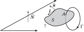
Figure 1: The circuit $\gamma$ and the closed path $\Gamma$ used to evaluate the circulation of $\mathbf{B}_{\gamma}$.

References

(1)R. P. Feynman, R. B. Leighton, and M. Sands, The
Feynman Lectures on Physics (Addison-Wesley, Reading,
MA, 1999), Vol. 2.
(2) J. D. Jackson, Classical Electrodynamics (John Wiley
Sons, New York, 1998), 3rd ed.
(3) S. M. Blinder, “Delta functions in spherical coordinates and how to avoid losing them: Fields of point charges and dipoles,” Am. J. Phys. 71, 816–818 (2003).
(4) B. D. H. Tellegen, “Magnetic-dipole models,” Am. J. Phys. 30, 650–652 (1962).
(5) N. D. Rao, “A note on the vector potential of a magnetic dipole,” Am. J. Phys. 39, 1276–1277 (1971).
(6) We use rationalized cgs units.
(7) I. M. Gel’fand and G. E. Shilov, Generalized
Functions (Academic Press, New York, 1964), Vol. 1.
(8) J. I. Richards and H. K. Youn The Theory of Distributions A Nontechnical Introduction (Cambridge University Press, 1995)
(9) H. B. G. Casimir, On the Interaction Between the Atomic Nuclei and Electrons (W. H. Freeman, San Francisco, 1963).
(10) D. J. Griffiths, “Hyperfine splitting in the ground state of hydrogen,” Am. J. Phys. 50, 698–703 (1982).
(11) More precisely, we deal with tempered distributions. Richards