PIC simulations of the Thermal Anisotropy-Driven Weibel Instability: Field growth and phase space evolution upon saturation

Abstract

The Weibel instability is investigated with PIC simulations of an initially unmagnetized and spatially uniform electron plasma. This instability, which is driven by the thermally anisotropic electron distribution, generates electromagnetic waves with wave vectors perpendicular to the direction of the higher temperature. Two simulations are performed: A 2D simulation, with a simulation plane that includes the direction of higher temperature, demonstrates that the wave spectrum is initially confined to one dimension. The electric field components in the simulation plane generated by the instability equalize at the end of the simulation through a secondary instability. A 1D PIC simulation with a high resolution, where the simulation box is aligned with the wave vectors of the growing waves, reveals details of the electron phase space distribution and permits a comparison of the magnetic and electric fields when the instability saturates. It is shown that the electrostatic field is driven by the magnetic pressure gradient and that it and the magnetic field redistribute the electrons in space.

1 Introduction

The filamentation instability or beam-Weibel instability has been proposed as a mechanism to magnetize the early universe [1, 2, 3, 4, 5, 6], to provide the strong magnetic fields for the afterglow emission of gamma-ray bursts [7, 8, 9, 10] and supernova explosions [11] and to explain the heating processes in the pulsar winds [12, 13]. It is also important for the inertial confinement fusion in laser-plasmas [14]. The filamentation instability has been investigated analytically [17, 7, 15, 16], numerically [18, 19] and also in a laboratory experiment [11], where it has been discussed as the precursor to the formation of astrophysical shocks of gamma-ray bursts and supernovae.

However, the filamentation instability is not the only instability that can generate magnetic fields. Here, we focus on a second one, the thermal anisotropy-driven Weibel instability (TAWI), which we study with particle-in-cell simulations. There are several analytical and numerical works of the TAWI, e. g. [13, 20, 21, 22, 23, 24]. We illustrate the physical mechanism behind the TAWI for a plasma, in which the temperature along one direction exceeds significantly those along the other two directions. The typical microcurrents of the electrons are highest along the direction with the high temperature. The magnetic interaction force that causes the deflection of electrons is thus strong orthogonal to this direction. At the same time, the typical particle’s thermal energy orthogonal to the direction with the high temperature is relatively weak. The particle’s thermal motion can, in this case, not oppose the structure formation. Current channels form with an axis, which is aligned with the direction of the high plasma temperature.

The original work of Weibel [25] considers a bi-Maxwellian distribution with one component of lower temperature yielding a one dimensional wave growth with wave vectors $\mathbf{k}$ in the direction of lower temperature. In contrast, we choose only one hot direction. The wave growth will then occur in the two dimensional plane perpendicular to that direction and give rise to the generation of a magnetic field in this plane.

The temperature anisotropy we consider here can be the result of a Buneman instability [26], which emerges for example at the terrestrial foreshock [27]. The latter is a result of the backstreaming of solar wind particles, which do not pass the terrestrial bow shock and move back into the solar wind domain. The backstreaming particles form a foreshock upstream of the shock. A Buneman instability develops between the shock-reflected ions and the electrons of the solar wind, if we assume for simplicity that no magnetic field is present. The phase velocity of the waves is comparable to the ion beam velocity [28], which we denote here as $v_{b}$ in the electron rest frame. The electric field amplitude grows and the electrons are trapped in phase space holes, when the kinetic energy of the electrons in the wave frame is not sufficient to escape the wave potential [29, 30]. They are accelerated along the beam velocity vector to a few times the beam speed. Since the spectrum of the waves driven by the Buneman instability is not strictly mono-directional, the electrons also experience a, usually weaker, acceleration away from the beam velocity vector. After the heating of the electrons, the Buneman instability is quenched. The electrons are heated more in the ion beam direction than in the plane orthogonal to it and a temperature anisotropy has developed.

The proximity of the terrestrial foreshock permits a direct access by in-situ observations. Therefore the particle configurations are well-known and the ion beam velocity could be determined to some hundred km$/$s [27], which is comparable to the speed of the Solar wind in the reference frame of the bow shock. We assume that this physical scenario can be applied to the foreshocks of supernova remnants (SNR), where the bulk flow speed of the supernova blast shell and thus of the SNR shock has been determined to be less or equal to $0.2c$ [31]. The ion beam speed should be similar to the velocity of the shock in the upstream reference frame.

Realistic values for the interstellar medium, into which a SNR shock is expanding, would be $B_{ISM}=1$ nT and $n_{ISM}\approx 1\textnormal{ cm}^{-3}$ [33], which would give a ratio of the plasma frequency to the electron cyclotron frequency of $\approx 300$. Thus, we can neglect the magnetic fields. Experimental evidence indicates that the magnetic field close to SNR shocks is amplified to values $\approx 100$ nT, presumably by the shock-accelerated cosmic ray particles [34, 35]. Recent PIC simulations [36] seem to suggest though, that the magnetic field cannot be amplified by the cosmic rays to values much higher than the amplitude of the background magnetic field.

The TAWI we consider here is driven by the electron heating by the shock-reflected ion beam, which we find even at unmagnetized shocks [37]. It can thus amplify a magnetic field from fluctuation levels and constitute the first stage of a chain of magnetic field amplification mechanisms upstream of a SNR shock. Our PIC simulations evidence that the peak magnetic field, which results from the TAWI, would be 8 nT for a plasma density of $1\textnormal{ cm}^{-3}$, well in excess of the ISM magnetic field. These 8 nT constitute a minimum estimate, because the electron density, which scales this peak field, is higher in the foreshock than in the ISM.

We perform two simulations and compare them to [22]: First we choose a 2D simulation plane that includes the direction of higher temperature, which we refer to as the parallel direction, and one perpendicular direction with a lower temperature. We show that the wave spectrum is one-dimensional during the early stage of the instability. In reality, this wave spectrum would be spread out over the plane that is orthogonal to the parallel direction. The dimensional reduction is, however, beneficial for the study of the interplay of the electromagnetic fields and the key plasma structures. We discuss the temporal behaviour of the electric and magnetic energy densities and analyse the field data, demonstrating that only that component of the magnetic field is amplified, which points out of the simulation plane. The magnetic pressure gradient generates initially an electric field in the perpendicular direction. A secondary instability transfers electric field energy from the perpendicular into the parallel direction.

Second we perform a 1D simulation along the perpendicular direction. We demonstrate that a weak electric field in the parallel direction is generated by Ampere’s law. The connection between the much stronger electric field in the perpendicular direction and the magnetic pressure gradient is demonstrated also in this setting. The growing magnetic field pushes the electrons together, yielding an increasingly complex layered structure in the velocity distribution.

The paper is structured as follows. The initial conditions and the simulation setup are given in the section 2. The results of the 2D and 1D simulations are presented in the sections 3 and 4, respectively. Section 5 discusses the results and the future work.

2 The instability, the initial conditions and the simulation method

2.1 The linear instability

We discuss the TAWI for electrons in a homogeneous, collisionless plasma and leave the ions as neutralising immobile background, which is equivalent to an infinitely large ion mass ($m_{i}\rightarrow\infty$). The plasma is initially unmagnetized ($B_{0}=0$). A temperature anisotropy $A=(v_{th\parallel}/v_{th\perp})^{2}-1>0$ in the electron particle distribution

$$f_{0}(v_{\perp},v_{\parallel})=\frac{1}{\pi^{3/2}c^{3}v_{th\perp}^{2}v_{th\parallel}}\exp\left[-\left(\frac{v_{\perp}^{2}}{v_{th\perp}^{2}}+\frac{v_{\parallel}^{2}}{v_{th\parallel}^{2}}\right)\right]$$ (1)

leads to growing electromagnetic oscillations with a wave vector $\mathbf{k}$ perpendicular to the direction of higher temperature. The velocities are normalized to the speed of light $c$.

We denote the direction of high temperature as the $x$-direction ($v_{th\parallel}=v_{thx}$). Hence, the wave growth of the TAWI mode can occur in the $y$-$z$ plane. We can limit our analysis to the $y$-direction due to the isotropy in this plane ($v_{th\perp}=v_{thy}$), accordingly $v_{th\perp}<v_{th\parallel}$.

The chosen thermal velocities are $v_{th\perp}=8.83\cdot 10^{-3}$ and $v_{th\parallel}=8.83\cdot 10^{-2}$, yielding $A=99$. The parallel thermal velocity is a few percent of the speed of light, which matches with the ion beam speed upstream of the SNR shocks. The perpendicular electron thermal velocity corresponds to a thermal energy of 40 eV.

The dispersion relation for the linear phase of the instability [38, 22]

$$k^{2}+\sigma^{2}=-\left[1+\frac{1}{2}(A+1)Z^{\prime}\left(\frac{\imath\sigma}{kv_{th\perp}}\right)\right]$$ (2)

describes the growth of the electromagnetic oscillations with a wave number $k$ in units of the inverse electron skin depth $\omega_{p}/c$ and its associated linear growth rate $\sigma$ in units of $\omega_{p}$. The frequency is purely imaginary ($\omega=\imath\sigma$), thus the oscillations do not propagate in space and grow exponentially in time. The electron plasma frequency for the number density $n_{e}$ is given by $\omega_{p}=(e^{2}n_{e}/\epsilon_{0}m_{e})^{1/2}$ and $Z^{\prime}(\zeta)=-2[1+\zeta Z(\zeta)]$ is the first derivative of the plasma dispersion function $Z(\zeta)=\pi^{-1/2}\int_{-\infty}^{\infty}dt\,\exp(-t^{2})/(t-\zeta)$.

Figure 1: The growth rate $\sigma(k)$. After a steep rise at low wave numbers the maximum is reached. Thermal effects limit the growth rate at large $k$. The wave number cutoff is given by $A^{1/2}$.

The plasma system is unstable for wave numbers in the range $0<k<k_{max}$ as depicted by the Fig. 1, where $k_{max}=A^{1/2}$ depends on the temperature ratio $T_{\parallel}/T_{\perp}>1$. The instability generates a magnetic field in perpendicular direction $B=B_{\perp}=(B_{y}^{2}+B_{z}^{2})^{1/2}$ and an electric field in parallel direction $E=E_{\parallel}=E_{x}$. The connection between $E$ and $B$ is given by the Maxwell relation $\mathbf{k}\times\mathbf{E}=\omega\,c\,\mathbf{B}$.

2.2 The simulation method and parameters

The PIC simulation is a method to model self-consistently the interplay of the electric and magnetic fields with the particles of a collision-less kinetic plasma [39]. The plasma is treated as an incompressible phase space fluid, which is approximated by an ensemble of volume elements. The Vlasov equation is solved by the method of characteristics, i. e. a Lorentz equation of motion is solved for each volume element. A volume element contains a large number of physical particles, which are treated as one computational particle (CP) with the same charge to mass ratio as the physical particles. The velocity of a CP is $\mathbf{v}_{cp}$ at the position $\mathbf{x}_{cp}$. With the relativistic momentum $\mathbf{p}_{cp}=m_{cp}\gamma\mathbf{v}_{cp}$ that is given in terms of $m_{e}c$ and $m_{cp}$ in terms of the electron mass $m_{e}$, the normalized Maxwell equations for the electric and magnetic fields $\mathbf{E}(\mathbf{x},t)$ and $\mathbf{B}(\mathbf{x},t)$

$$\nabla\times\mathbf{E}=-\frac{\partial\mathbf{B}}{\partial t},\,\,\nabla\times\mathbf{B}=\frac{\partial\mathbf{E}}{\partial t}+\mathbf{J},$$ (3)

and the normalized Lorentz equation

$$\frac{\textnormal{d}\mathbf{p}_{cp}}{\textnormal{d}t}=q_{cp}(\mathbf{E}[\mathbf{x}_{cp}]+\mathbf{v}_{cp}\times\mathbf{B}[\mathbf{x}_{cp}])$$ (4)

are solved. The quantities $\mathbf{E}$ and $\mathbf{B}$ can be transformed to physical units by a multiplication by $\omega_{p}m_{e}/ce$ and $\omega_{p}m_{e}/e$, respectively. The normalized current density $\mathbf{J}$ is transformed to physical units by a multiplication with $cn_{e}e$. The $q_{cp}$ is given in units of the elementary charge $e$ and the simulation time $t$ and position $\mathbf{x}$ are given in units of $1/\omega_{p}$ and $c/\omega_{p}$, respectively. The code fulfills $\nabla\cdot\mathbf{E}=\rho/\epsilon_{0}$ and $\nabla\cdot\mathbf{B}=0$ to round-off precision [40].

The current $\mathbf{J}$, the electric and the magnetic fields are defined on a grid. The electromagnetic fields are interpolated from the grid to the position of each CP. The momentum of the CP is updated with these interpolated fields and with the Lorentz equation of motion. The new particle position is calculated with the old particle position, $\mathbf{v}_{cp}$ and the time step $\Delta_{t}$. The microcurrents $\propto q_{cp}\mathbf{v}_{cp}$ are the contributions of each discrete particle, i. e. the CPs in our simulations or the electrons in a real physical plasma. They are interpolated from each CP back onto the grid and by integrating over all CPs the total current $\mathbf{J}$ is obtained. Then the electric and magnetic fields are updated with (3) and the individual steps are repeated.

Our PIC simulations represent either one or two spatial dimensions and all components of $\mathbf{p}_{cp}$. The boundary conditions are periodic in all directions. The quadratic 2D simulation box employs an equal number of cells $N_{x}=N_{y}=1000$ in the $x$- and in the $y$-direction, each with a side length $\Delta_{x}\omega_{p}/c=8.4\times 10^{-3}$. The number of CPs per cell is $N_{2}=150$. For the 1D simulation we use $N_{y}=1000$ cells in the $y$-direction, $N_{x}=1$ and the same $\Delta_{x}$. The number of CPs per cell is in this case $N_{1}=32768$. The time step is given by $\Delta_{t}\omega_{p}\approx 3.9\cdot 10^{-3}$. The equations solved by the PIC code are given in normalized units and they can be scaled to any value of the plasma frequency. We choose a reference value for the plasma frequency ($\omega_{p}=6.3\cdot 10^{5}\textnormal{ s}^{-1}$) to illustrate the field amplitudes in physical units.

3 Two-dimensional simulation

3.1 The electric and magnetic energy densities

The box-averaged energy densities of the electric $E_{i}(x,y,t)$ and magnetic $B_{i}(x,y,t)$ field components are given by $\epsilon_{Ei}(t)=(N_{x}\,N_{y})^{-1}\sum\limits_{j,k}\epsilon_{0}{\left[E_{i}(j\Delta_{x},k\Delta_{x},t)\right]}^{2}/2$ and $\epsilon_{Bi}(t)=(N_{x}\,N_{y})^{-1}\sum\limits_{j,k}{\left[B_{i}(j\Delta_{x},k\Delta_{x},t)\right]}^{2}/2\mu_{0}$, respectively. The box-averaged kinetic energy density is $\epsilon_{K}(t)=(N_{x}\,N_{y})^{-1}\Delta_{x}^{-3}\sum\limits_{j}m_{cp}\,c^{2}(\gamma_{j}-1)$, where the summation is over the $N_{y}\,N_{1}$ or $N_{x}N_{y}\,N_{2}$ particles for the 1D or the 2D simulation, respectively. The only magnetic field component that grows in the considered geometry in response to the TAWI is the $B_{z}$ component, which is confirmed by the PIC simulations.

Fig. 2 demonstrates that the energy density of $B_{z}$ increases exponentially first and saturates for large simulation times similar to [22]. The electric field component $E_{y}$ is also amplified. The energy density of $E_{y}$ does not grow in the 2D box at twice the exponential rate, with which the energy density of $B_{z}$ is growing. It does so only in the 1D simulation (shown here for comparison, Fig. 2(b)).

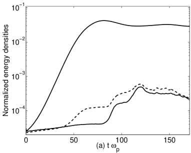
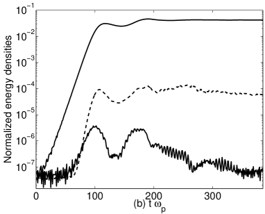
Figure 2: 10-logarithmic plot of the ratios $\epsilon_{Bz}/\epsilon_{K}(t=0)$ (upper solid), $\epsilon_{Ey}/\epsilon_{K}(t=0)$ (dashed) and $\epsilon_{Ex}/\epsilon_{K}(t=0)$ (lower solid) for the 2D (a) and 1D simulation (b). The TAWI amplifies $B_{z}$, which induces a component $E_{y}$. In 2D $E_{x}$ is amplified later than $E_{y}$ and their energies eventually equalize.

The growth of the component $E_{x}$ is delayed with respect to $E_{y}$. Eventually, both components $E_{x}$ and $E_{y}$ reach the same energy density in Fig. 2(a). In reference [22] the electric energy density is just a horizontal line because the energy densities have been plotted on a linear scale. The energy densities of the other field components did not grow during the simulation time.

3.2 The field evolution

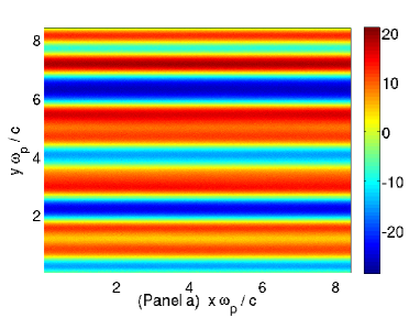
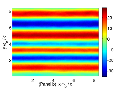
Figure 3: The magnetic field component $cB_{z}$ at the simulation times $t\omega_{p}=59$ (a) and $t\omega_{p}=164$ (b). The colourbar denotes the value in V/m (colours online). After the onset of the amplification of $E_{x}$ the filaments are not strictly one-dimensional anymore.

Fig. 3 displays the magnetic field component $cB_{z}$ at the simulation times $t\omega_{p}=59$ and $t\omega_{p}=164$. The left panel shows the magnetic field component $cB_{z}$ at the time when $E_{y}$ saturates first. The component $E_{x}$ has not been amplified yet. Magnetic filaments have developed with a symmetry axis parallel to the $x$-direction. The right panel displays the magnetic field component when both electric field components have reached almost the same amplification level. The magnetic field structures are not strictly parallel to the $x$-axis anymore (e. g. at $y\omega_{p}/c=6.5$), but they remain qualitatively unchanged in the considered reduced geometry. The structures would merge if the two perpendicular directions would be resolved [22].

The mechanism that transfers the electric field energy density from the $E_{y}$ to the $E_{x}$ component is revealed by comparing the spatial field profiles before and after the growth of $E_{x}$ in the Fig. 4.

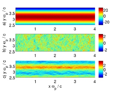
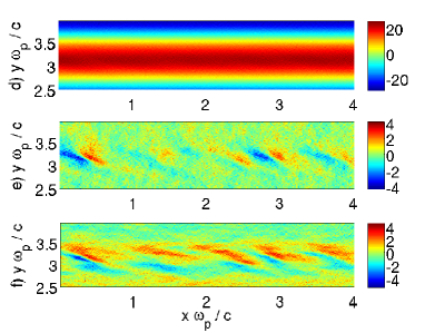
Figure 4: The relevant field components at two times in a box sub-interval in units of V/m (colours online): The $cB_{z}$, $E_{x}$ and $E_{y}$ components at $t\omega_{p}=75$ are shown in the panels a,b,c, respectively. The panels d,e,f display the $cB_{z}$, $E_{x}$ and $E_{y}$ components at $t\omega_{p}=87$, respectively.

The $E_{y}$-component is practically uniform along $x$ and the structures are parallel to those of $cB_{z}$ at $t\omega_{p}=75$ and both are likely to be correlated. The amplitude $E_{y}$ performs a full oscillation in the spatial interval $2.6<y\omega_{p}/c<3.6$ between two zero-crossings of $cB_{z}$. No significant structures can be seen in $E_{x}$ at this time. The $cB_{z}$ component is qualitatively unchanged in the time interval $75<t\omega_{p}<87$ also on this scale, but the oscillation amplitude along $y$ decreases somewhat. The electric field does, however, undergo a drastic change. The $E_{y}$ that is initially uniform along $x$ becomes oscillatory at the later time. One oscillation takes place on a distance $0.8c/\omega_{p}$ along $x$, which corresponds to the wavenumber $k_{x}c/\omega_{p}\approx 8$, as can be seen best from the $E_{y}$ component. The oscillations along $x$ rotate the electric field polarization vector away from $y$ at $t\omega_{p}=87$.

The observed spatial periodicity along $x$ is evidence for a secondary instability, possibly a sausage mode instability [43]. It is this instability that couples the energy from the $E_{y}$ component into the $E_{x}$ component (see Fig. 2). This is confirmed by the supplementary movie 1, which animates in time the 10-logarithmic spatial power spectrum ${|\tilde{E}(k_{x},k_{y})|}^{2}$ of $\tilde{E}(x,y)=E_{x}(x,y)+iE_{y}(x,y)$. The movie 1 demonstrates that the electric field power is concentrated at $k_{x}\approx 0$ until $t\omega_{p}\approx 80$, which is equivalent to a spatially uniform electric field along $x$. A signal grows after $t\omega_{p}\approx 80$ at $k_{x}c/\omega_{p}\approx 8$, which corresponds to the oscillation of $E_{y}$ in the Fig. 4(f). This signal is spread over a wide band of $k_{y}$. Initially this signal grows only in the quadrant $k_{x},k_{y}>0$, but it rapidly spreads out in the wavenumber space after $t\omega_{p}\approx 100$. In [22] this secondary instability was not observed as only the magnetic field has been analyzed.

3.3 The electron phase space distribution

The variation of $B_{z}$ along $y$ must be supported by a current component $J_{x}$ that varies along $y$. In order to obtain information about the distribution of the electrons in terms of the normalised momentum $p_{x}/m_{e}c$, we slice out 6 cells ($0.084\leq x\omega_{p}/c\leq 0.134$) in the $x$-direction and integrate the phase space density over this $x$ interval to improve the particle statistics. We compare the electron phase space distribution $f(y,p_{x})$ to $J_{x}(y)$.

Fig. 5 displays $f(y,p_{x})$ and $J_{x}(y)$ for the two simulation times corresponding to Fig. 3. At $t\omega_{p}=59$ the mean momentum of the bulk electrons changes piecewise linearly with $y$ and it spans a range $|p_{x}/m_{e}|\apprle v_{th\parallel}$. This results in a piecewise change of the current $J_{x}$. The $B_{z}(y)$ is consequently varying quadratic over extended $y$ intervals (not shown). At $t\omega_{p}=164$ these phase space structures become more diffuse. The magnetic field amplitude in Fig. 3 decreases by the reduction of $J_{x}$ at late times and, consequently, the energy density of $B_{z}$ in the Fig. 2(a).

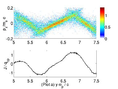
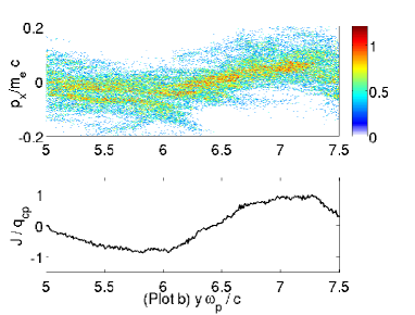
Figure 5: Top: The 10-logarithmic momentum distribution $f(y,p_{x})$ at the simulation times $t\omega_{p}=59$ (left) and $t\omega_{p}=164$ (right) (colours online): The structure of the electron phase space distribution is initially an approximately piecewise linear function of $y$. The structure is diffuse at late times. Bottom: $J_{x}(y)/q_{cp}$ at $t\omega_{p}=59$ (left) and $t\omega_{p}=164$ (right). The current initially varies piecewise linearly with $y$. It is smoothened at late times and its amplitude has decreased.

4 One-dimensional simulation

We examine now with such a 1D simulation the time beyond $t\omega_{p}\approx 50$, when the TAWI grows the $E_{y}$ field. The one-dimensional geometry suppresses $E_{x}$.

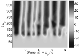
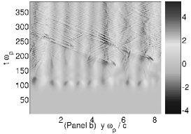
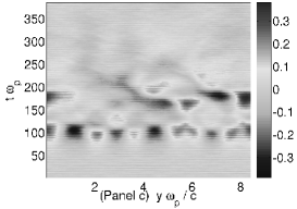
Figure 6: The development of the field components $cB_{z}$, $E_{y}$ and $E_{x}$ during the simulation. The colourbar denotes the value in V$/$m. (a): The magnetic field structure is quasi-static and oscillatory in space. (b): $E_{y}$ has a double frequency compared with $cB_{z}$. Fast waves appear for $t\omega_{p}>180$. (c): The low frequency waves of $E_{x}$ are generated by Ampere’s law with a resulting phase shift of $90^{\circ}$ towards $B_{z}$.

As in the 2D simulation only the $z$-component of the magnetic field has developed. The magnetic field structures are quasi-static and oscillatory in space (Fig. 6(a)). The structure of $E_{y}$ in Fig. 6(b) has the half wavelength of $cB_{z}$ like in Fig. 3(a). For $90\leq t\omega_{p}\leq 180$ the structure is time-independent. This stationarity is an artifact of the 1D geometry. It permits us to separate the effects of $E_{x}$ and $E_{y}$ on the electrons, which simplifies their interpretation. For $t\omega_{p}>180$ fast waves appear in $E_{y}$, which are superposed on the periodic structure. Their velocity $v\approx c/20$ is of the order of $v_{th\parallel}$.

The $E_{x}$ in Fig. 6(c) resembles $cB_{z}$ for $t\omega_{p}<120$ and has an amplitude that is one order of magnitude below that of $E_{y}$. Eq. (3), which is in one dimension $\partial_{y}B_{z}=\partial_{t}E_{x}+J_{x}$, implies that a growing $J_{x}$ generates the oscillations of $E_{x}$. The phase shift of $90^{\circ}$ between $cB_{z}$ and $E_{x}$ shown in Fig. 6 is an evidence for this connection. The oscillations of $E_{x}$ correspond to transient waves and they damp out as evidenced also by Fig. 2(b).

Movie 2 shows the evolution of the electron charge density and the field components $cB_{z}$ and $E_{y}$. Initially, the growth of the $cB_{z}$ and $E_{y}$ components reveals a spatial correlation and the electron charge density is modulated accordingly. Oscillations of the electron charge density and of the $E_{y}$ component with a short wavelength develop at late times. These rapid spatial oscillations obscure the long spatial oscillations. The latter are, however, still present, as the Fig. 6 demonstrates for $E_{y}$. The oscillation of $B_{z}$ with the initial wavenumber remains dominant.

In Fig. 7 snapshots are taken and the connection with the phase space distribution is investigated. In the 1D simulation the electrons can move freely only along the $y$-direction. The TAWI generates initially a zigzag distribution, which yields through its currents the growth of the magnetic field. The amplitude of the velocity oscillations upon saturation are comparable to $v_{th\parallel}$, which is clearly recognizable at $t\omega_{p}=96$ (See left column of Fig. 7 and movie 3). The wave number of $E_{y}$ is twice that of $cB_{z}$ at this time and the zero crossings of $E_{y}$ coincide with the extrema and zero crossings of $cB_{z}$. At this stage the magnetic field still grows exponentially. Forces due to $E_{y}$ and $v_{cp}B_{z}$ are not yet strong enough to affect the electron trajectories. Until strong electromagnetic fields have developed, the electrons perform just a thermal motion in the $y$-direction. Once the electromagnetic fields become strong at $t\omega_{p}=116$, they push together the particles along the $y$-direction, yielding a layered structure in the phase space distribution (middle column Fig. 7). The complexity of the phase space distribution increases further with the time, which is evident from the movie 3 and the right column in Fig. 7. The fine structure at the beginning of the simulation thermalizes but the zigzag distribution of the bulk remains. This holds up the currents which are neccessary to support the magnetic field. A coalescence of the filaments is not apparent.

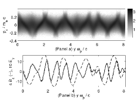
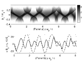
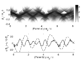
Figure 7: Row a: $f(y,p_{x})$ of the particles at $t\omega_{p}=96$ (left), $t\omega_{p}=116$ (middle) and $t\omega_{p}=154$ (right). The colourbar denotes the 10-logarithm of the number of CPs. Row b: $cB_{z}$ (dashed) and $10E_{y}$ (solid) at the times corresponding to the electron distributions above. The $y$-axis denotes the value in V/m.

In order to demonstrate quantitatively the link between the magnetic pressure gradient and $E_{y}$, these are plotted in Fig. 8(a). The expected proportionality of the magnetic pressure gradient and the electric field

$$-eE_{y}(y)=n_{e}^{-1}\,\partial_{y}P_{b}(y)=n_{e}^{-1}\mu_{0}^{-1}B_{z}(y)\,\partial_{y}B_{z}(y)$$ (5)

had to be modified by a factor 2. This factor can be understood as follows. The magnetic pressure gradient force accelerates the electrons, giving rise to a $J_{y}\neq 0$. The $J_{y}$ is tied through Ampère’s law to an $E_{y}$ and the phases of both are shifted in time by $90^{\circ}$. Initially, $E_{y}=0$ and $J_{y}=0$ and $E_{y}$ must thus oscillate around an electric field set. The peak value of $E_{y}$ is given by the added fields of the oscillatory $E_{y}$ and of this set. This amounts to twice the amplitude of the set electric field, which is determined by the magnetic pressure gradient force.

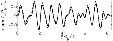
Figure 8: The normalized magnetic pressure gradient $2\partial_{y}P_{b}/n_{e}e$ (solid) and the negative electric field component $-E_{y}$ (dashed) in values of V/m at $t\omega_{p}=96$.

Fig. 9 analyses the electron distribution and the fields in a subsection of the simulation box at the time $t\omega_{p}=96$. The electron phase space distribution follows the zigzag distribution. The width of the distribution in $p_{x}$ with more than 300 particle counts is practically constant along $y$ on the linear and 10-logarithmic density scales. The thermal spread and the electron density increase somewhat at the breaks, which coincide with the zero-crossings of $E_{y}$ and $cB_{z}$.

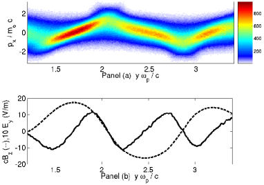
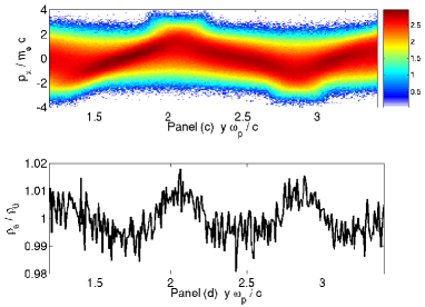
Figure 9: The electron distribution and the electromagnetic fields in a sub-interval of the box at $t\omega_{p}=96$ (colours online). (a) The electron phase space density in units of a CP on a linear scale. The density decreases from the center outwards. (b) The electrostatic field $10E_{y}$ (solid) and the $cB_{z}$ (dashed) due to the TAWI. (c) The 10-logarithmic electron phase space density in units of a CP. (d) The electron charge density normalized to its mean value.

A comparison of the Figs. 9(a,b,d) reveals the cause of the density accumulation and the zigzag distribution. Let us consider the interval to the right of the break at $y\omega_{p}/c\approx 2.1$. There, the electron bulk has a $p_{x}>0$ and the $E_{y},B_{z}<0$. The $E_{y}<0$ implies that the electrons accelerate away from the break in the direction of increasing $y$. The electrons accelerate away from the break also for the interval just to the left of $y\omega_{p}/c=2.1$, where $E_{y}>0$. The break is thus an unstable equilibrium in what the $E_{y}$ driven by $\nabla P_{b}$ is concerned and it cannot explain the electron accumulation close to $y\omega_{p}/c=2.1$ in Fig. 9(d). This is accomplished by the $B_{z}$. The Lorentz force component along $y$ due to $B_{z}$ for a computational electron with $q_{cp}<0,v_{cp,x}>0,B_{z}<0$ just to the right of $y\omega_{p}/c=2.1$ is $F_{cp}=-q_{cp}v_{cp,x}B_{z}<0$ and the electron is accelerated towards $y\omega_{p}/c=2.1$. The particles are also accelerated towards the break just to the left of it, because $B_{z}$ changes its sign. It is thus the drift electric field $\propto v_{x}B_{z}$ that compresses the electrons. The electrostatic force that is due to the magnetic pressure gradient, which oscillates twice as fast as $B_{z}$ along $y$, opposes this compression close to the break and enforces it further away. The force contribution by the electrostatic field is not negligible. The peak speed along $x$ of the electrons is $0.1c$ and the Lorentz force $v\times B$ is thus comparable to that due to $E_{y}$.

5 Discussion

In this work we have examined the thermal anisotropy-driven Weibel instability (TAWI). We have limited our investigation to an unmagnetized, non-relativistic plasma, considering only the electron dynamics and neglecting the ions. The TAWI is driven by a temperature anisotropy in the electron distribution. Here, the direction of higher temperature has been aligned with the $x$-direction. Thus, the TAWI modes would have wave vectors in the plane orthogonal to $x$.

We have performed two simulations. The first one is a 2D simulation in the $x$-$y$-plane. As the electrons can move freely only in this plane, the waves that grow due to the TAWI are planar with a wave vector along $y$. Second we have performed a 1D simulation along $y$ with a large number of computational particles per cell. This has enabled through an increased dynamical range the identification of fine structure in the electron phase space distribution and it has reduced the noise. Both simulations have not resolved the $y$-$z$-plane, which would be necessary to enable the interplay of the current filaments [22]. We can thus separate the dynamics of individual current filaments driven by the TAWI from their mutual nonlinear interactions, as in [22], and leave the latter to future work.

As expected, only the $z$-component of the magnetic energy density has been amplified [22]. After an initial exponential growth phase of $B_{z}$, the wave has saturated. The growth of $B_{z}$ has been accomplished by the turning of the initially spatially uniform electron velocity distribution into a zigzag distribution in the phase space. The mean speed along $x$ varies for this distribution piecewise linearly as a function of $y$. The initial $J_{x}(y)=0$ is thus transformed into a $J_{x}(y)\neq 0$ in most parts of the simulation box. In both simulations the saturation resulted in the growth of an electrostatic $E_{y}$ component. We have demonstrated with the 1D simulation the link between this $E_{y}$ and the force due to the magnetic pressure gradient $\nabla P_{b}$. This connection was qualitatively unchanged in the 2D simulation, but the box-averaged electrostatic energy density did not grow at twice the exponential rate of the $B_{z}$, as in the 1D simulation of the TAWI and in simulations of the filamentation instability [41, 44, 18]. The $E_{x}$ component could grow to a high amplitude only in the 2D simulation. The $E_{x}$ in the 1D simulation has been driven by the growing $J_{x}$ according to Ampere’s law but only to a low amplitude. These modes damped out rapidly. The stronger $E_{x}$ in the 2D simulation developed in response to a secondary instability, probably a sausage instability [43]. The 1D simulation cannot resolve this instability, because it involves wavevectors along $x$.

The 1D PIC simulation provided an insight into the link between the fields and the electron phase space structures and it could resolve the charge density oscillations that developed during the nonlinear stage of the TAWI. The breaks in the zigzag distribution have been examined in more detail. The breaks correspond to the positions, at which the change with $y$ of the mean momentum along $x$ reverses its sign. The charge density and the electron temperature are increased at the breaks and the amplitudes of $E_{y},B_{y}$ have zero-crossings. The $E_{y}$ field accelerates electrons away from the break, while the drift electric field imposed by the non-zero mean speed along $x$ and the $B_{z}$ is compressing the electrons along $y$. This compression is stronger close to the breaks than the electric repulsion, which results in an electron accumulation.

We have demonstrated that the force due to the electric field is comparable to the Lorentz force imposed by the magnetic field, because the electron speeds are only a few per cent of the light speed. The focus on the magnetic forces and the neglection of the electric ones in Ref. [22] may thus not always be justified for the Weibel instability. The high phase space resolution of PIC simulations, which is now possible, has revealed that the size of the filaments in the 1D simulation increases not through the merger of filaments, which is inhibited by the 1D geometry, but through a broadening of the filaments due to the overlap of phase space layers. The filament mergers suggested by Fig. 3 in Ref. [22] could be an artifact of the lower plasma resolution or from the display of phase space slices instead of the full distribution. This has to be investigated with a future simulation that employs the anisotropy $A=24$ of Ref. [22].

The connection of the magnetic and electric fields driven by the TAWI thus resembles those reported for the filamentation instability, which is driven by counterpropagating electron beams. Stable plasmons developed in [44] after the filamentation instability has saturated, which were confined by the potential due to the drift electric field and the magnetic pressure gradient. Here, the electron phase space distribution in the 1D simulation developed fine structures first evolving into a thermalized distribution with a bulk zigzag distribution.

We will investigate in future work the statistical properties of the TAWI in 1D and in 2D, as it has been done for the filamentation instability [42, 45]. Ultimately, a 3D simulation has to be performed as in Ref. [23], which considered the original Weibel instability in which the electrons are hot along two cartesian directions and cool along the third. These simulations may provide an insight into the scale size and field strength of the magnetic field structures that develop out of nonthermal electron distributions in astrophysical flows and to what extent these structures could be responsible for the frequently observed synchrotron radiation.

Acknowledgements: This work was partially supported by the Forschergruppe 1048 of the Deutsche Forschungsgemeinschaft through grant Schl201/21-1. ME Dieckmann has been financed by Vetenskapsrådet and through the grant FOR1048 of the Deutsche Forschungsgemeinschaft. We thank the HPC2N supercomputer centre for the computer time and support. The Workshop “PIC Simulations of Relativistic Collisionless Shocks” in Dublin, Ireland (May 19 – 23, 2008) provided us with helpful suggestions.

References

References

- [1] Gruzinov A 2001 Astrophys. J. 563 L15
- [2] Okabe N and Hattori M 2003 Astrophys. J. 599 964
- [3] Schlickeiser R and Shukla P K 2003 Astrophys. J. 599 L57
- [4] Schlickeiser R 2005 Plasma Phys. Controll. Fusion 47 A205
- [5] Fujita Y and Kato T N 2005 Mon. Not. R. Astron. Soc. 364 247
- [6] Medvedev M V, Silva L O and Kamionkowski M 2006 Astrophys. J. 642 L1
- [7] Achterberg A and Wiersma J 2007 A&A 475 1
- [8] Medvedev M V and Loeb A 1999 Astrophys. J. 526 697
- [9] Waxman E 2006 Plasma Phys. Controll. Fusion 48 B137
- [10] Spitkovsky A 2008 Astrophys. J. 673 L39
- [11] Medvedev M V 2007 Astrophys. and Space Science 307 245
- [12] Yang Y T B, Gallant Y, Arons J and Langdon A B 1993 Phys. Fluids B 5 3369
- [13] Arons J 2008 AIPC 983 200
- [14] Tabak M, Callahan-Miller D, Ho D D-M and Zimmerman G B 1998 Nucl. Fusion 38 509
- [15] Pétri J and Kirk J G 2007 Plasma Phys. Controll. Fusion 49 1885
- [16] Tautz R C and Schlickeiser R 2006 Phys. Plasmas 13 062901
- [17] Yoon P H and Davidson R C 1987 Phys. Rev. A 35 2718
- [18] Stockem A, Dieckmann M E and Schlickeiser R 2008 Plasma Phys. Controll. Fusion 50 025002
- [19] Silva L O, Fonseca R A, Tonge J W, Dawson J M, Mori W B and Medvedev M V 2003 Astrophys. J. 596 L121
- [20] Schaefer-Rolffs U and Schlickeiser R 2006 Phys. Plasmas 13 012107
- [21] Schlickeiser R 2004 Phys. Plasmas 11 5532
- [22] Morse R L and Nielsen C W 1971 Phys. Fluids 14 830
- [23] Romanov D V, Bychenkov V Y, Rozmus W, Capjack C E, and Fedosejevs R 2004 Phys. Rev. Lett. 93 215004
- [24] Pukhov A 2001 Phys. Rev. Lett. 86 3562
- [25] Weibel E S 1959 Phys. Rev. Lett. 2 83
- [26] Ishihara O, Hirose A and Langdon A B 1980 Phys. Rev. Lett. 44 1404
- [27] Eastwood J P, Lucek E A, Mazella C, Meziane K, Narita Y, Pickett J and Treumann R A 2005 Space Sci. Rev. 118 41
- [28] Buneman O 1958 Phys. Rev. Lett. 1 8
- [29] Roberts H L and Berk K V 1967 Phys. Rev. Lett. 19 297
- [30] Dieckmann M E, Ljung P, Ynnerman A and McClements K G 2000 Phys. Plasmas 7 5171
- [31] Kulkarni S R, Frail D A, Wieringa M H, Ekers R D, Sadler E M, Wark R M, Higdon J L, Phinney E S and Bloom J S 1998 Nature 395 663
- [32] Goldstein M L, Eastwood J P, Treumann R A, Lucek E A, Pickett J and Decreau P 2005 Space Sci. Rev. 118 7
- [33] Ellison D C and Vladimirov A 2008 ApJL 673 L47
- [34] Volk H J, Berezhko E G, Ksenofontov L T 2005 Astron. Astrophys. 433 229
- [35] Bell A R 2004 MNRAS 353 550
- [36] Niemiec J, Pohl M, Stroman T, Nishikawa K 2008 ApJ 684 1174
- [37] Forslund D W and Shonk C R 1970 PRL 25 1699
- [38] Lazar M, Smolyakov A, Schlickeiser R and Shukla P K 2008 J. Plasma Phys. 75 19
- [39] Dawson J M 1983 Rev. Mod. Phys. 55 403
- [40] Eastwood J W 1991 Comput. Phys. Comm. 64 252
- [41] Califano F, Cecchi T and Chiuderi C 2002 Phys. Plasmas 9 451
- [42] Rowlands G, Dieckmann M E and Shukla P K 2007 New J. Phys. 9 247
- [43] Das A, Jain N, Kaw P and Sengupta S 2004 Nucl. Fusion 44 98
- [44] Dieckmann M E, Rowlands G, Kourakis I and Borghesi M 2008 arXiv:0810.5267v1 [physics.plasm-ph]
- [45] Dieckmann M E, Lerche I, Shukla P K and Drury L O C 2007 New J. Phys. 9 10