RU-NHETC-2009-01

On mass spectrum in ’t Hooft’s
2D model of mesons

V. A. Fateev^1,3, S. L. Lukyanov^2,3 and

A. B. Zamolodchikov^2,3

¹ Laboratoire de Physique Th${\acute{\rm e}}$orique et Astroparticules

UMR5207 CNRS-UM2, Universit${\acute{\rm e}}$ Montpellier II

Pl. E. Bataillon, 34095 Montpellier, France

²NHETC, Department of Physics and Astronomy

Rutgers University

Piscataway, NJ 08855-0849, USA

³L.D. Landau Institute for Theoretical Physics

Chernogolovka, 142432, Russia

Abstract

We study ’t Hooft’s integral equation determining the meson masses $M_{n}$ in multicolor QCD₂. In this note we concentrate on developing an analytic method, and restrict our attention to the special case of quark masses $m_{1}=m_{2}=g/\sqrt{\pi}$. Among our results is systematic large-$n$ expansion, and exact sum rules for $M_{n}$. Although we explicitly discuss only the special case, the method applies to the general case of the quark masses, and we announce some preliminary results for $m_{1}=m_{2}$ (Eqs. (6.1) and (6.3)).

 

May 2009

1 Introduction

As was discovered by G. ’t Hooft in 1974 [1], the mass spectrum of mesons in multi-color QCD in two dimensions admits for exact solution, because in this model the mesons are essentially the two-body constructs, and their masses are exactly determined by the Bethe-Salpeter equation. For the mesons built from two quarks of bare (lagrangian) masses $m_{1}$ and $m_{2}$, the Bethe-Salpeter equation reduces to the singular integral equation

$$2\pi^{2}\,\lambda\ \ \varphi(x)=\bigg{[}\,{{\alpha_{1}}\over{x}}+{{\alpha_{2}}\over{1-x}}\,\bigg{]}\,\varphi(x)-\ \mathchoice{{\vbox{\hbox{$\textstyle-$}}\kern-4.86108pt}}{{\vbox{\hbox{$\scriptstyle-$}}\kern-3.25pt}}{{\vbox{\hbox{$\scriptscriptstyle-$}}\kern-2.29166pt}}{{\vbox{\hbox{$\scriptscriptstyle-$}}\kern-1.875pt}}\!\int_{0}^{1}{\rm d}y\ {{\varphi(y)}\over{(y-x)^{2}}}\ ,$$ (1.1)

where

$$\alpha_{1}=\frac{\pi m_{1}^{2}}{g^{2}}-1\,,\qquad\alpha_{2}=\frac{\pi m_{2}^{2}}{g^{2}}-1\,,$$ (1.2)

with $g$ being the ’t Hooft coupling constant (which in $2D$ has the dimension of mass). The function $\varphi(x)$ has to satisfy the boundary conditions

$$\varphi(0)=\varphi(1)=0\,,$$ (1.3)

whence Eq.(1.1) defines the spectral problem for the parameter $\lambda$; the eigenvalues $\lambda_{n},n=0,1,2,...$ are discrete, and determine the meson masses,

$$M_{n}^{2}=2\pi g^{2}\ \lambda_{n}\,.$$ (1.4)

In principle, the problem can be solved numerically, to any degree of accuracy, and over the years a number of approaches were developed to that end [1, 2, 3, 4, 5]. However, we believe equation (1.1) deserves further study from an analytical standpoint. In our opinion, the most interesting problem with respect to Eq.(1.1) is understanding the analytic properties of the eigenvalues $\lambda_{n}$ as the functions of complex $\alpha_{1}$ and $\alpha_{2}$. Without significant analytic input, straightforward numerical approaches seem to be unsuitable to addressing this problem. At the same time, the neat form of equation (1.1) suggests that perhaps some analytic information can be extracted.

In this note we report new results about the spectrum $\{\lambda_{n}\}$ in the special case

$$\alpha_{1}=\alpha_{2}=0\,.$$ (1.5)

Among our results is systematic semiclassical (large-$n$) expansion of the eigenvalues,

$$2\lambda_{n}=n+{\textstyle\frac{3}{4}}-\frac{2}{3\pi^{6}\,(n+\frac{3}{4})^{3}}+\frac{2\ (-1)^{n+1}}{\pi^{4}\,(n+\frac{3}{4})^{2}}\,\bigg{\{}1-\frac{4\log\big{[}\pi\text{e}^{\gamma_{E}-{1\over 2}}\,(n+{\frac{3}{4}})\big{]}}{\pi^{2}\,(n+\frac{3}{4})}\,\bigg{\}}+O\big{(}{\textstyle{\frac{\log^{2}(n)}{n^{4}}}}\big{)}.$$ (1.6)

Here $\gamma_{E}$ is the Euler constant and we display just three leading terms, but in principle any number of terms can be produced via our technique (next four terms can be deduced from (4.25), (4.27), (4.28) and equations (7), (7) in Appendix A). Note the unusual logarithmic factors in the third and higher terms, which make this expansion look rather different from the standard WKB expansion in the Schr$\ddot{\rm o}$dinger problem. In addition, our approach allows for analytic evaluation of the spectral sums

$$G^{(s)}_{+}=\sum_{m=0}^{\infty}\,\frac{1}{\lambda_{2m}^{s}}\,,\qquad\quad G^{(s)}_{-}=\sum_{m=0}^{\infty}\,\frac{1}{\lambda_{2m+1}^{s}}$$ (1.7)

with integer $s=2,\,3,\,4,\,\ldots$ . (The sums here are over even or odd eigenvalues. The corresponding eigenstates are even or odd with respect to obvious $x\to 1-x$ symmetry of (1.1).) For low $s$ we have, explicitly

$$G^{(2)}_{+} = 7\,\zeta(3)\,,\qquad\qquad\qquad\qquad\ G^{(2)}_{-}=2\,,$$

$$G^{(3)}_{+} = -{\textstyle{4\over 3}}\,\pi^{2}+28\,\zeta(3)\,,\qquad\qquad\,G^{(3)}_{-}=-{\textstyle{8\over 3}}+{\textstyle{4\over 9}}\,\pi^{2}\,,$$

$$G^{(4)}_{+} = -2\pi^{2}+42\,\zeta(3)-{\textstyle{7\over 3}}\ \pi^{2}\,\zeta(3)+{\textstyle{49\over 2}}\ \zeta^{2}(3)+{\textstyle{31\over 2}}\ \zeta(5)\,,$$

$$G^{(4)}_{-} = {\textstyle{11\over 3}}-{\textstyle{7\over 9}}\ \pi^{2}+{\textstyle{7\over 6}}\ \pi^{2}\,\zeta(3)-{\textstyle{31\over 4}}\ \zeta(5)\,.$$

Again, in principle analytic expressions for any given $s$ can be obtained, but for larger $s$ the calculations become increasingly involved. At the moment we have these numbers up to $s=13$, but only those with $s=5,\,\ldots\,8$ have sufficiently compact form to be presented in Appendix A. Put together, the large-$n$ expansion (1.6) and the sum rules (1.7) provide good control over the entire spectrum: the large-$m$ parts of the sums (1.7) can be approximated by the asymptotic expansions (1.6), thus providing equations for the lower eigenvalues.

We regard this work as preparatory for studying the spectrum of (1.1) with arbitrary $\alpha_{1}$, $\alpha_{2}$, with the aim of understanding analytic properties of the eigenvalues at complex values of these parameters. We concentrate here on developing the technique, and the case (1.5) is convenient for testing its efficiency. Besides, many details have particularly neat form in this case. But for the most part, our technique admits more or less straightforward extension to the general case, which will be the next stage of this project. The method also seems to be suitable for analysis of a large class of Bethe-Salpeter equations of the type of (1.1) which emerge in many $2D$ field theories with confining interactions.

The paper is organized as follows. In Section 2 we discuss general properties of Eq.(1.1). In particular we relate its solutions to solutions of a certain functional equation (see Eq.(2.6)) of the type of Baxter’s $T-Q$ equation, with special analyticity. In Section 3 we develop $\lambda$-series expansion of the solutions of this equation. This expansion generates analytic expressions for the spectral sums (1.7). Asymptotic expansion at $\lambda\to\infty$ is developed in Section 4. It results in the large-$n$ expansion of the eigenvalues $\lambda_{n}$. In Section 5 we test these results against the numerical solution of (1.1).

While this paper was in preparation, we have made some progress in studying the more general case of (1.1), with nonzero but equal values of the parameters

$$\alpha_{1}=\alpha_{2}=\alpha\,.$$ (1.9)

We intend to devote a separate paper to discussing this more general case, where indeed a very interesting analytic structure of $\lambda_{n}(\alpha)$ emerges. But we could not resist the temptation to announce some results here, which are presented in Section 6.

2 Functional equation

We find it useful to recast Eq.(1.1) into somewhat different form, via the integral transformation

$$\varphi(x)=\int_{-\infty}^{\infty}{{\rm d}\nu\over 2\pi}\ \Psi(\nu)\ \big{(}{\textstyle{x\over 1-x}}\big{)}^{\frac{{\rm i}\nu}{2}}\,,\quad\Psi(\nu)=\int_{0}^{1}{{\rm d}x\over 2x(1-x)}\ \ \varphi(x)\ \big{(}{\textstyle{x\over 1-x}}\big{)}^{-\frac{{\rm i}\nu}{2}}\,,$$ (2.1)

which is just Fourier transform with respect to the variable $\frac{1}{2}\,\log(\frac{x}{1-x})$ (This transformation was previously used in Ref.[8]). The $\nu$-space form of (1.1) is

$$\nu\,\coth\big{(}{\textstyle\frac{\pi\nu}{2}}\big{)}\ \Psi(\nu)-\lambda\,\int_{-\infty}^{\infty}{\rm d}\nu^{\prime}\ S(\nu-\nu^{\prime})\ \Psi(\nu^{\prime})=0\,,$$ (2.2)

where the kernel

$$S(\nu)=\frac{\pi\nu}{2\,\sinh(\frac{\pi\nu}{2})}$$ (2.3)

in the right hand side is regular at all real $\nu$. The solution $\Psi(\nu)$ must decay at $|\nu|\to\infty$ (for the norm $\parallel\varphi\parallel^{2}=\int_{0}^{1}{\rm d}x\ |\varphi(x)|^{2}$ to be finite), and it must be a smooth function of $\nu$ (for the function $\varphi(x)$ in (1.1) to satisfy the boundary conditions (1.3)). The spectrum $\{\lambda_{n}\}$ is determined by the existence of solutions which satisfy these conditions. In fact, both these conditions, once satisfied, are satisfied with substantial redundancy.

Equation (2.2) dictates that any smooth solution is in fact analytic. Moreover, it is possible to show that the solutions $\Psi(\nu)$ are meromorphic functions of $\nu$, with the poles at $\nu=\pm(2k-1)\,{\rm i}$, $k\in\mathbb{Z}$, of the order $k\in{\mathbb{N}}$. In particular, the function $Q(\nu)$ defined as

$$Q(\nu)=\nu\,\cosh\big{(}{\textstyle\frac{\pi\nu}{2}}\big{)}\ \Psi(\nu)$$ (2.4)

is analytic in the strip $|\Im m\,\nu|\leq 2$, grows slower then any exponential of $\nu$ at infinity, and turns to zero at $\nu=0,\,\pm 2{\rm i}$, i.e.

$$Q(0)=Q(\pm 2{\rm i})=0\,.$$ (2.5)

Under these conditions the integral operator in the right hand side can be inverted in terms of finite difference operator (which is derived by standard manipulations with shifts of the integration contour), leading to the functional equation

$$Q(\nu+2{\rm i})+Q(\nu-2{\rm i})-2\,Q(\nu)=-4\pi\lambda\ \ \nu^{-1}\,\tanh\big{(}{\textstyle\frac{\pi\nu}{2}}\big{)}\ Q(\nu)\,.$$ (2.6)

Equation (2.6) is the basis of our analysis below.

A quick look at the asymptotic form of (2.6) at $\Re e\,\nu\to\infty$ reveals that its solutions generally behave as ${\rm e}^{k\,\nu}\,f(\nu)$, with integer $k$, and $f(\nu)$ bounded by any exponential. Obviously, any positive $k$ would violate the asymptotic condition for $\Psi(\nu)$. Thus, we are interested in the solutions which are bounded as

$$Q(\nu)=O\big{(}\,{\rm e}^{\epsilon|\nu|}\,\big{)}\qquad\text{as}\quad|\Re e\,\nu|\to\infty\,,$$ (2.7)

with any $\epsilon$. Note that this condition implies that the function $\Psi(\nu)$ in fact decays exponentially in this limit.

A solution of (2.6) with the desired analytic and asymptotic properties exists only at specific values of $\lambda$, which determine the eigenvalues of (2.2). However, if the conditions (2.5) are relaxed, the solutions $Q(\nu|\lambda)$ exist at any $\lambda$. For generic $\lambda$, the associated function $\Psi(\nu|\lambda)$ no longer satisfies the integral equation (2.2). Instead, it solves the related inhomogeneous equation

$$\nu\,\coth\big{(}{\textstyle\frac{\pi\nu}{2}}\big{)}\ \Psi(\nu|\lambda)-\lambda\ \mathchoice{{\vbox{\hbox{$\textstyle-$}}\kern-4.86108pt}}{{\vbox{\hbox{$\scriptstyle-$}}\kern-3.25pt}}{{\vbox{\hbox{$\scriptscriptstyle-$}}\kern-2.29166pt}}{{\vbox{\hbox{$\scriptscriptstyle-$}}\kern-1.875pt}}\!\int_{-\infty}^{\infty}{\rm d}\nu^{\prime}\ S(\nu-\nu^{\prime})\ \Psi(\nu^{\prime}|\lambda)=F(\nu|\lambda)\,,$$ (2.8)

where

$$F(\nu|\lambda)=\frac{q_{+}(\lambda)\,\nu+q_{-}(\lambda)}{\sinh({\pi\nu\over 2})}\,,$$ (2.9)

with the coefficients $q_{+}(\lambda)$ and $q_{-}(\lambda)$ related to the values $Q(0|\lambda)$ and $Q(\pm 2{\rm i}|\lambda)$ in a linear manner (note that in view of the functional equation (2.6), only two of these values are independent). Since now in general $Q(0|\lambda)\neq 0$, the integrand in the l.h.s. involves a first order pole at $\nu^{\prime}=0$, and the integral is understood as its principal value. It is possible to show that, given the coefficients $q_{\pm}$, the solution of (2.8) is unique. These coefficients can be chosen at will, and therefore the equation (2.8) generates two-dimensional space of functions $\Psi(\nu|\lambda)$. It is natural to choose the basis in accord with the obvious $\nu\to-\nu$ symmetry of the problem. We thus define symmetric and antisymmetric basic functions,

$$\Psi_{\pm}(-\nu|\lambda)=\pm\,\Psi_{\pm}(\nu|\lambda)\,,$$ (2.10)

which solve the equation (2.8) with $F(\nu|\lambda)$ in the r.h.s. taken to be

$$F_{+}(\nu)=\frac{\nu}{\sinh(\frac{\pi\nu}{2})}\qquad\text{and}\qquad F_{-}(\nu)=\frac{1}{\sinh(\frac{\pi\nu}{2})}\ ,$$ (2.11)

respectively.

At the spectral points $\lambda=\lambda_{n}$ the original equation (2.2) is to be recovered. That means that at certain values of $\lambda$ the basic functions $\Psi_{\pm}(\nu|\lambda)$ diverge. More precisely, Eq. (2.8) can be rewritten in the form of an inhomogeneous Fredholm integral equation of the second kind (see Appendix B for details) and it follows from the resolvent formalism that $\Psi_{\pm}(\nu|\lambda)$ are meromorphic functions of $\lambda$, with only poles at the eigenvalues of (2.2),

$$\Psi_{+}(\nu|\lambda)=\sum_{m=0}^{\infty}\frac{{\rm c}_{2m}\Psi_{2m}(\nu)}{\lambda-\lambda_{2m}}\,,\quad\quad\Psi_{-}(\nu|\lambda)=\sum_{m=0}^{\infty}\ \frac{{\rm c}_{2m+1}\Psi_{2m+1}(\nu)}{\lambda-\lambda_{2m+1}}\ ,$$ (2.12)

where, as we have mentioned in Introduction, $\lambda_{2m}$ and $\lambda_{2m+1}$, $m=0,\,1,\,2,\ldots$, refer to the eigenvalues of (2.2) in the even and odd sectors, respectively, and $\Psi_{2m}(\nu)$ and $\Psi_{2m+1}(\nu)$ are associated eigenfunctions.

It is useful to note that the functions $\Psi_{+}(\nu|\lambda)$ and $\Psi_{-}(\nu|\lambda)$ are related to the “quark form factors” of the vector current $J_{\mu}={\bar{\psi}}\gamma_{\mu}\psi$ and the scalar density $S={\bar{\psi}}\psi$, respectively, with the parameter $\lambda$ (more precisely $2\pi\,g^{2}\,\lambda$) interpreted as $q^{2}$, the square of the total 2-momentum (see Refs.[9, 10], where inhomogeneous integral equations equivalent to (2.8), (2.11) appear in this connection). Therefore the structure (2.12) is well expected, and the coefficients ${\rm c}_{n}$ in (2.12) are related to the matrix elements

$$\langle\,0\mid\,J_{\mu}(0)\,\mid M_{2m},q\,\rangle = {\rm i}\ \epsilon_{\mu\nu}\,q^{\nu}\ \sqrt{N_{c}}\ \pi^{3\over 2}\ \ {\rm c}_{2m}\ ,$$ (2.13)

$$\langle\,0\mid S(0)\mid M_{2m+1},q\,\rangle = 2\pi g\ \ \sqrt{N_{c}}\ \ {\rm c}_{2m+1}\ ,$$

where $\mid M_{n},q\,\rangle$ stands for the $n$-th meson state with 2-momentum $q$. Let us mention here the neat expressions for the current-current correlation function in terms of $\Psi_{+}(\nu|\lambda)$,

$$\langle\,J_{\mu}(q)\,J_{\nu}(-q)\,\rangle={{\rm i}N_{c}\over\pi}\ \Big{(}\,\frac{q_{\mu}q_{\nu}}{q^{2}}-g_{\mu\nu}\Big{)}\ \big{[}\,1-\Psi_{+}(0|\lambda)\,\big{]}\ .$$ (2.14)

Having in mind this analyticity in $\lambda$, our strategy in solving the problem will be as follows. Starting with equation (2.6), we will be looking for two solutions, $Q_{+}(\nu|\lambda)$ and $Q_{-}(\nu|\lambda)$ of the functional equation (2.6), analytic in the strip $|\Im m\,\nu|\leq 2$, and growing slower than any exponential at $|\Re e\,\nu|\to\infty$. We will assume that

$$Q_{\pm}(-\nu|\lambda)=\mp\,Q_{\pm}(\nu|\lambda)\,,$$ (2.15)

and fix the normalizations by the conditions

$$Q_{+}(2{\rm i}|\lambda)=-Q_{+}(-2{\rm i}|\lambda)=2{\rm i}\,,\qquad Q_{-}(0|\lambda)=1\,.$$ (2.16)

Then the functions $\Psi_{\pm}(\nu|\lambda)$ related to $Q_{\pm}(\nu|\lambda)$ as in (2.4) have appropriate symmetry (2.10), and solve the equation (2.8) precisely with the right-hand sides (2.11), as one can readily verify. In fact, the remarkably simple formula

$$\partial_{\lambda}\log D_{\pm}(\lambda)=2{\rm i}\,\partial_{\nu}\ \log Q_{\mp}(\nu|\lambda)\big{|}_{\nu={\rm i}}$$ (2.17)

relates the logarithmic derivatives of $Q_{\mp}$ at $\nu={\rm i}$ to suitably defined spectral determinants,

$$D_{+}(\lambda)=\prod_{m=0}^{\infty}\bigg{(}1-\frac{\lambda}{\lambda_{2m}}\bigg{)}\ {\rm e}^{\frac{\lambda}{\lambda_{2m}}}\,,\qquad D_{-}(\lambda)={\rm e}^{2\lambda}\,\prod_{m=0}^{\infty}\bigg{(}1-\frac{\lambda}{\lambda_{2m+1}}\bigg{)}\ {\rm e}^{\frac{\lambda}{\lambda_{2m+1}}}\,.$$ (2.18)

(To be precise, somewhat more complicated expressions, Eqs. (8.20), follow directly from the integral equation (2.8). See Appendix B, where we explain the status of Eq. (2.17).) Note that this relation is insensitive to normalization conditions assumed for $Q_{\pm}(\nu|\lambda)$. In what follows, we develop two different expansions for such solutions $Q_{\pm}(\nu|\lambda)$. One is just the power series in $\lambda$, and the other is the asymptotic expansion around the essential singularity $\lambda=\infty$. Eq.(2.17) translates the former expansions into the sum rules (1.7), while the latter ones lead to the large-$n$ expansion (1.6).

Before turning to the details, let us make the following remark. The functional equation (2.6) has the form of the famous $T-Q$ relation of Baxter, and many general statements can be adopted to our case. In particular, it is easy to show that the so-called quantum Wronskian built from the two solutions $Q_{\pm}(\nu|\lambda)$ is a constant,

$$Q_{+}(\nu+{\rm i}|\lambda)\,Q_{-}(\nu-{\rm i}|\lambda)-Q_{+}(\nu-{\rm i}|\lambda)\,Q_{-}(\nu+{\rm i}|\lambda)=2{\rm i}\ .$$ (2.19)

The fact that this combination does not depend on $\nu$ follows from the functional equation (2.6), and the asymptotic conditions at $|\Re e\,\nu|\to\infty$. The particular value $2{\rm i}$ in the r.h.s. reflects the special normalization (2.16); with different normalization it would be a different (generally $\lambda$-dependent) constant. This equation, combined with (2.17), allows one to establish some useful relations. It follows from (2.17) that $Q_{+}({\rm i}|\lambda)$ turns to zero at the odd spectral values $\lambda=\lambda_{2m+1}$ (likewise, $Q_{-}({\rm i}|\lambda)$ does the same at the even values $\lambda_{2m}$). But the identity $Q_{+}({\rm i}|\lambda)\,Q_{-}({\rm i}|\lambda)={\rm i}$ (elementary consequence of (2.19)) shows that $\lambda_{2m+1}$ exhaust all zeros of $Q_{+}({\rm i}|\lambda)$ viewed as the function of $\lambda$. In other words, $Q_{+}({\rm i}|\lambda)$ must be proportional to $D_{-}(\lambda)/D_{+}(\lambda)$, up to a factor which is entire function of $\lambda$ with no zeros, i.e. in our case the factor of the form $\exp(a+b\lambda)$. More careful analysis (in the next section) allows one to fix this ambiguity completely. Let us present here the result in the form

$$\frac{Q_{+}({\rm i}|\lambda)}{Q_{+}(2{\rm i}|\lambda)}={{1\over 2}}\ \frac{D_{-}(\lambda)}{D_{+}(\lambda)}\,,\quad\ \ \ \ \frac{Q_{-}({\rm i}|\lambda)}{Q_{-}(0|\lambda)}=2{\rm i}\ \frac{D_{+}(\lambda)}{D_{-}(\lambda)}\,,$$ (2.20)

insensitive to normalizations of $Q_{\pm}(\nu|\lambda)$.

3 Expansion in powers of $\lambda$

In principle, one can generate the expansion in $\lambda$ just by iterating the integral equation (2.8), with the right-hand side taken in one of the forms (2.11) (see Eqs. (8.14) in Appendix B). This leads to the convergent series

$$Q_{\pm}(\nu|\lambda)=\sum_{s=0}^{\infty}Q_{\pm}^{(s)}(\nu)\ \lambda^{s}\,,$$ (3.1)

with the coefficients given by $s$-fold integrals involving the kernel $S(\nu)$. Direct evaluation of these integrals is difficult, and therefore we take another approach based on the functional equation (2.6). We look for the solution of (2.6) in the form of the power series (3.1), with the coefficients $Q_{\pm}^{(s)}(\nu)$ having the symmetry (2.15), analytic in the strip $|\Im m\,\nu|\leq 2$, and growing slower than any exponential at $|\Re e\,\nu|\to\infty$. It is clear upfront that at each order these conditions fix the coefficients uniquely (after all, it is just a somewhat indirect way of evaluating the integrals appearing in the iterative solution of (2.8)). But the solution for $Q_{\pm}^{(s)}(\nu)$ obtained this way involves polynomials of $\nu$ of growing degree, and the expressions quickly become cumbersome. The following observation greatly facilitates the calculations.

Note that the factor

$$z\equiv 2\pi\lambda\,\tanh\big{(}{\textstyle\frac{\pi\nu}{2}}\big{)}$$ (3.2)

in the r.h.s. of this equation, is insensitive to the shifts $\nu\to\nu\pm 2{\rm i}$, and if no attention to the analytic properties is paid, it can be regarded as constant. Then the equation (2.6), written as

$$Q(\nu+2{\rm i})+Q(\nu-2{\rm i})-2\,Q(\nu)=-2z\ \nu^{-1}\,Q(\nu)$$ (3.3)

is recognizable as one of the recursion relations satisfied by confluent hypergeometric functions [13]. Specifically, the functions $\nu\,M(1+{{\rm i}\nu\over 2},2,-{\rm i}z)$ and $\Gamma(1+{{\rm i}\nu\over 2})\,U(1+{{\rm i}\nu\over 2},2,-{\rm i}z)$ are known to satisfy (3.3) (see e.g. [13], Eqs. 13.4.1, 13.4.15). Here the conventional notations $M(a,c,x)$ and $U(a,c,x)$ for two canonical solutions of confluent hypergeometric equation are used. Of course, by themselves these functions do not provide solution to our problem, since they have wrong analyticity in $\nu$. For one, the second of these functions has logarithmic singularity at $z=0$, which in view of (3.2) produces unpleasant branching points in the $\nu$-plane. This problem is easy to cure by observing that the logarithmic term by itself satisfies Eq.(3.3), and subtracting it produces another solution which is now a single-valued function of $\nu$. Thus, we found it convenient to use the combinations

$$M_{+}(\nu,z) = \nu\,{\rm e}^{{\rm i}z\over 2}\ M\big{(}1+{\textstyle\frac{{\rm i}\nu}{2}},\,2,-{\rm i}z\big{)}\,,$$ (3.4)

$$M_{-}(\nu,z) = -{\rm i}z\,{\rm e}^{{\rm i}z\over 2}\,\Gamma\big{(}1+{\textstyle\frac{{\rm i}\nu}{2}}\big{)}\,U\big{(}1+{\textstyle\frac{{\rm i}\nu}{2}},2,-{\rm i}z\big{)}-$$ (3.5)

$${\textstyle{1\over 2}}\,\big{[}\,z\,\log\big{(}-{\textstyle{{\rm i}\over 4}}\,z\,{\rm e}^{\gamma_{E}}\,\big{)}+{\rm i}\pi^{2}\lambda\,\big{]}\ {M}_{+}(\nu,z)\ ,$$

where the coefficients ${\rm e}^{{\rm i}z\over 2}$ and the extra constant in the brackets in (3.5) are chosen to ensure the symmetry

$$M_{\pm}(-\nu,-z)=\mp M_{\pm}(\nu,z)\,,$$ (3.6)

in accord with the obvious symmetry of Eq.(3.3). Both (3.4) and (3.5) are entire functions of $z$, in particular both can be represented by convergent expansions in the powers of $z$:

$$M_{+}(\nu,z) = \nu\,{\rm e}^{{\rm i}z\over 2}\ \sum_{s=0}^{\infty}{(1+{{\rm i}\nu\over 2})_{s}\over(s+1)!s!}\ \ (-{\rm i}z)^{s}\ ,$$ (3.7)

$$M_{-}(\nu,z) = {\textstyle{1\over 2}}\ \Big{[}\ {\rm e}^{{\rm i}z\over 2}\,\Sigma(\nu,z)+{\rm e}^{-{{\rm i}z\over 2}}\,\Sigma(-\nu,-z)\ \Big{]}\,,$$

where

$$\Sigma(\nu,z)=1+\sum_{s=1}^{\infty}{({{\rm i}\nu\over 2})_{s}\over s!(s-1)!}\ \Big{[}\,\psi\big{(}s+{\textstyle{{\rm i}\nu\over 2}}\big{)}-\psi(s)-\psi(s+1)+\psi\big{(}{\textstyle{1\over 2}}\big{)}\,\Big{]}\,\ (-{\rm i}z)^{s}\ .$$ (3.8)

These expansions make explicit a more serious problem. In view of (3.2), each term of this expansion produces poles at $\nu=\pm\,{\rm i}$, of growing order, and thus both (3.4) and (3.5), viewed as the functions of $\nu$ at fixed $\lambda$, have essential singularities at these points, whereas we need solutions of (2.6) analytic in the strip $|\Im m\,\nu|\leq 2$. We are thus compelled to look for the solutions in the form

$$Q_{\pm}(\nu|\lambda)=A_{\pm}(z,\lambda)\ M_{\pm}(\nu,z)+B_{\pm}(z,\lambda)\ z\,M_{\mp}(\nu,z)\ ,$$ (3.9)

where the coefficients, entire functions of $z^{2}$, are to be adjusted to compensate for the above singularity at $z=\infty$. So far we were unable to find the closed form solution of this analytic problem. But it is easy to generate the solution as an expansion in the powers of $\lambda$. In view of the above analyticity, we assume that the coefficients can be expanded in double series in $\lambda$ and $z^{2}$. Regarding them as the functions of $\nu$ and $\lambda$ (through the relation (3.2)), this expansions has the form of the power series

$$A_{\pm}(z,\lambda)=\sum_{s=0}^{\infty}\,a_{\pm}^{(s)}(\tau)\,\lambda^{s}\,,\qquad\qquad B_{\pm}(z,\lambda)=\sum_{s=0}^{\infty}\,b_{\pm}^{(s)}(\tau)\,\lambda^{s}$$ (3.10)

with $a_{\pm}^{(s)}(\tau)$ and $b_{\pm}^{(s)}(\tau)$ being polynomials in $\tau\equiv({z\over 4\lambda})^{2}={\pi^{2}\over 4}\tanh^{2}(\frac{\pi\nu}{2})$, of the highest degree $[s/2]$. The numerical coefficients in these polynomials are to be adjusted in such a way as to compensate for all the pole terms generated by the expansions of the functions $M_{\pm}(\nu,z)$ in (3.9), order by order in $\lambda$. The remaining constant terms are then fixed by the normalization conditions (2.16) which demand that $A_{\pm}(0,\lambda)=1$. Clearly, this linear problem at each order has a unique solution. We have calculated explicitly the polynomials $a_{\pm}^{(s)}(\tau)$, $b_{\pm}^{(s)}(\tau)$ up to $s=13$. Let us present here the first few of them, just to give the flavor of it:

$$a^{(2)}_{+}=\tau\,,\qquad\qquad a^{(3)}_{+}={\textstyle{64\over 9}}\,\tau\,,\qquad a^{(4)}_{+}={\textstyle{1\over 4}}\ \tau\ \big{(}\,50+21\,\zeta(3)-5\tau\,\big{)}\,,$$

$$b_{+}^{(0)}={\textstyle{1\over 2}}\,,\qquad\qquad b^{(1)}_{-}={\textstyle{4\over 3}}\,,\qquad\ \ \ \ b^{(2)}_{-}={\textstyle{1\over 4}}\ \big{(}\,6+7\,\zeta(3)-\tau\,\big{)}\,,$$ (3.11)

and

$$a^{(2)}_{-}=-\tau\,,\qquad\ a^{(3)}_{-}={\textstyle{8\over 9}}\,\tau\,,\qquad\ \ \ a^{(4)}_{-}={\textstyle{1\over 12}}\ \tau\ \big{(}\,21\,\zeta(3)-14+3\tau\,\big{)}\,,$$

$$b_{-}^{(0)}=0\,,\qquad\ \ \ \ b^{(1)}_{-}=4\,,\qquad\qquad b^{(2)}_{-}={\textstyle{7\over 2}}\,\zeta(3)-5-\tau\,.$$ (3.12)

Eq.(2.17) makes it straightforward to convert the $\lambda$-expansions of $Q_{\pm}(\nu|\lambda)$ into the expansions of the spectral determinants (2.18),

$$\log D_{\pm}(\lambda)=(1\mp 1)\,\lambda-\sum_{s=2}^{\infty}\,s^{-1}\ G_{\pm}^{(s)}\ \lambda^{s}\,,$$ (3.13)

where the coefficients give explicitly the spectral sums (1.7). For the few lowest $s$ the result of this calculation was already displayed in (1), but we present many more in Appendix A. With many $G^{(\pm)}_{s}$ known, the sum rules (1.7) become a useful tool in determining the eigenvalues $\lambda_{n}$, especially so when combined with the large-$n$ asymptotic expansions, which we derive in the next section.

4 Asymptotic expansion at $\lambda\to\infty$

To develop the large-$\lambda$ expansions of the functions $Q_{\pm}(\nu|\lambda)$ we start by constructing a formal solution of the functional equation (2.6), of the following structure

$$S(\nu|\lambda)=(-\lambda)^{-\frac{{\rm i}\nu}{2}}\ \sum_{k=0}^{\infty}\,S_{k}(\nu)\,{\lambda^{-k}}\,.$$ (4.1)

It is impossible to satisfy all the analytic conditions required for the functions $Q_{\pm}(\nu|\lambda)$ within this ansatz, but we would like to get as close to the desired analyticity as possible. In particular, we demand that the coefficients $S_{k}(\nu)$ are meromorphic functions of $\nu$, growing slower then any exponential at $|\Re e\,\nu|\to\infty$. The form (4.1) is obviously designed to serve the case of negative real $\lambda$, if we choose the principal branch of $(-\lambda)^{-\frac{{\rm i}\nu}{2}}$ (other branches exhibit unacceptable exponential growth at $|\Re e\,\nu|\to\infty$).

Plugging this expansion into (2.6) generates a sequence of recurrent functional equations for the coefficient functions $S_{k}(\nu)$. In the zeros order we have

$$S_{0}(\nu+2{\rm i})={\frac{4\pi}{\nu}}\,\tanh\Big{(}{\frac{\pi\nu}{2}}\Big{)}\ S_{0}(\nu)\,.$$ (4.2)

The solution of this equation, analytic in the strip $|\Im m\,\nu|\leq 2$ and bounded at $|\Re e\,\nu|\to\infty$, is unique up to a normalization. It can be written in an explicit form

$$S_{0}(\nu)=\left(2\pi\right)^{-{1\over 2}-\frac{{\rm i}\nu}{2}}\,\ \frac{G\left(2+\frac{{\rm i}\nu}{2}\right)\,G\left(\frac{1}{2}-\frac{{\rm i}\nu}{2}\right)}{G\left(1-\frac{{\rm i}\nu}{2}\right)\,G\left(\frac{3}{2}+\frac{{\rm i}\nu}{2}\right)}\ \ \ \ \ \ \ \ \ \ \ \ \big{(}\,S_{0}({\rm i})=1\,\big{)}$$ (4.3)

in terms of the Barnes $G$-function (see e.g. [14])

$$G(x+1)=(2\pi)^{x\over 2}\ {\rm e}^{-{x(x+1)\over 2}-{\gamma_{E}\over 2}\,x^{2}}\ \prod_{n=1}^{\infty}\bigg{[}\,\Big{(}1+{x\over n}\Big{)}^{n}\,{\rm e}^{-x+{x^{2}\over 2n}}\,\bigg{]}\ .$$ (4.4)

At higher orders in $\lambda^{-1}$ the equation (2.6) leads to the recurrent relations of the form

$$\sigma_{k}(\nu+2{\rm i})-\sigma_{k}(\nu)=\rho_{k}(\nu)$$ (4.5)

for the ratios $\sigma_{k}(\nu)=S_{k}(\nu)/S_{0}(\nu)$, with $\rho_{k}(\nu)$ being certain expressions involving $\sigma_{k^{\prime}}(\nu)$ from the lower orders $k^{\prime}=k-1,\,k-2$. While beyond the leading order no solutions analytic in the strip $|\Im m\,\nu|\leq 2$ exist, it is possible to find solutions analytic in that strip except for the points $\nu=0,\pm 2{\rm i}$, where the poles of growing order appear. The result of this calculation is summarized by the formula

$$S(\nu|\lambda)=R(z,\lambda)\,{\hat{U}}(\nu,z)\,,$$ (4.6)

where ${\hat{U}}(\nu,z)$ stands for the formal asymptotic series

$${\hat{U}}(\nu,z)=(-\lambda)^{-\frac{{\rm i}\nu}{2}}\ S_{0}(\nu)\ \sum_{k=0}^{\infty}\,\frac{\left(1+\frac{{\rm i}\nu}{2}\right)_{k}\,\left(\frac{{\rm i}\nu}{2}\right)_{k}}{k!}\ (\,{\rm i}z\,)^{-k}\,,$$ (4.7)

and $z$ is the same combination (3.2), insensitive to the shifts $\nu\to\nu\pm 2{\rm i}$. The fact that (4.7) satisfies (2.6) can be verified directly, but it is clear upfront from the following observation; The series appearing in (4.7), when multiplied by $\Gamma(1+{{\rm i}\nu\over 2})\ (-{\rm i}z)^{-1-{{\rm i}\nu\over 2}}$, coincides with the asymptotic expansion of the function $\Gamma(1+{{\rm i}\nu\over 2})\ U(1+{{\rm i}\nu\over 2},2,-{\rm i}z)$, which satisfies (2.6). In writing (4.7) we simply replaced the overall factor $\Gamma(1+{{\rm i}\nu\over 2})\ (-{\rm i}z)^{-1-\frac{{\rm i}\nu}{2}}$ by the much more analytically attractive $(-\lambda)^{-\frac{{\rm i}\nu}{2}}\ S_{0}(\nu)$. The factor $R(z,\lambda)$ in (4.6) represents the ambiguities in the solutions of (4.5); it is to be understood as a formal series in the powers of $z^{-1}$ and $\lambda^{-1}$, or equivalently as a series in $\lambda^{-1}$ with the coefficients being polynomials in the variable

$$c\equiv\,{\rm i}\pi\,\coth\big{(}{\textstyle\frac{\pi\nu}{2}}\big{)}\,.$$ (4.8)

The asymptotic expansions of the functions $Q_{\pm}(\nu|\lambda)$ can be built from the formal solution (4.7) in much the same way as the $\lambda$-expansions were constructed from the basic functions (3.4), (3.5) in the previous section. Having in mind the symmetry (2.15), we look for $Q_{\pm}(\nu|\lambda)$ in the form

$$Q_{\pm}(\nu|\lambda)\asymp R_{\pm}(z,\lambda)\,{\hat{U}}(\nu|z)\,\mp\,R_{\pm}(-z,\lambda)\,{\hat{U}}(-\nu|-z)\,.$$ (4.9)

The coefficients $R_{\pm}(z,\lambda)$ are to be adjusted to fix the analytic problems present in ${\hat{U}}(\nu|z)$ and ${\hat{U}}(-\nu|-z)$. One of these problems was already mentioned above. The series (4.7) explicitly exhibits at each order in $\lambda^{-1}$ poles at $\nu=0,\pm 2{\rm i}$, of the growing order. This problem can be fixed order by order in $\lambda^{-1}$, with $R_{\pm}(z,\lambda)$ taken in the form

$$R_{\pm}(z,\lambda)\propto 1+\sum_{k=1}^{\infty}\,R_{\pm}^{(k)}(c,L)\,\lambda^{-k}\,,$$ (4.10)

with $R_{\pm}^{(k)}(c,L)$, polynomials in the cotangent (4.8), adjusted to cancel these poles. Because of the factor $(-\lambda)^{-\frac{{\rm i}\nu}{2}}$, the Laurent expansions of (4.7) around the poles generate logarithms of $-\lambda$. As a result, the coefficients $R_{\pm}^{(k)}$ in (4.10) emerging in this calculation turn out to be also polynomials in the variable

$$L=\log\left(-2\pi\lambda\right)+\gamma_{E}\,.$$ (4.11)

This is a novel feature of the large-$\lambda$ expansion, which ultimately leads to the logarithmic factors in the expansions (1.6). As expected, the solution of this pole-cancellation problem at each order in $\lambda^{-1}$ turns out to be essentially unique, i.e. unique up to terms which can be absorbed into the overall normalization of $Q_{\pm}(\nu|\lambda)$. With the relations (2.20), the normalization conditions (2.16) imply the following general form of the coefficients $R_{\pm}(z,\lambda)$:

$$R_{\pm}(z,\lambda)=(-\lambda)^{-{1\over 2}}\ {\rm i}^{1\mp 1\over 2}\ \bigg{[}\,{D_{-}(\lambda)\over 2D_{+}(\lambda)}\,\bigg{]}^{\pm 1}\ \bigg{[}\,1+c\,\sum_{k=1}^{\infty}P^{(k)}_{\pm}(c,L)\ \lambda^{-k}\,\bigg{]}\ .$$ (4.12)

We have explicitly computed the polynomials $P_{\pm}^{(k)}(c,L)$ up to $k=7$, but display here only the first few of them (again, just to give the flavor of the emerging expressions):

$$P_{\pm}^{(1)}(c,L)=0\,,\qquad P_{\pm}^{(2)}(c,L)={{\pm 1\over 4\pi^{4}}}\,,\qquad P_{\pm}^{(3)}(c,L)={{\pm 1\over 24\pi^{6}}}\ (6\,c-12L+6\mp 1)\ .$$ (4.13)

The overall factors in (4.12) are related to the ratio of the spectral determinants (2.18) via (2.20); the expansion

$${D_{-}(\lambda)\over D_{+}(\lambda)}\asymp\sqrt{2\over-\lambda\pi^{2}}\ \exp\bigg{[}\,{1\over 2\lambda\pi^{2}}-{L\over 2(\lambda\pi^{2})^{2}}+{6L(L-1)-\pi^{2}-1\over 12(\lambda\pi^{2})^{3}}+O(L^{3}\lambda^{-4})\,\bigg{]}$$ (4.14)

is obtained in a straightforward way once $P^{(k)}_{\pm}(c,L)$ are determined, by imposing the normalization condition (2.16) order by order in $\lambda^{-1}$.

These results are readily applied, through Eq.(2.17), to write down the large-$\lambda$ expansions of the individual spectral determinants

$$\partial_{\lambda}\log D_{\pm}(\lambda)\asymp L-1+\log(4)+\frac{-1\pm 2}{8\,\lambda}-\pi^{2}\ \sum_{k=2}^{\infty}P^{(k)}_{\mp}(0,L)\ \lambda^{-k}\,,$$ (4.15)

where $L$ is the logarithm (4.11), and the terms $\propto\lambda^{-2}$ and higher involve the polynomials (4.13) specified to $c=0$. This equation determines the large-$\lambda$ expansions of $D_{\pm}(\lambda)$ up to an overall numerical factors

$$D_{\pm}(\lambda)\asymp d_{\pm}\,\big{(}8\pi{\rm e}^{-2+\gamma_{E}}\big{)}^{\lambda}\ (-\lambda)^{\lambda-\frac{1}{8}\,\pm\,\frac{1}{4}}\ \exp\bigg{[}\ \sum_{k=1}^{\infty}\,F_{\pm}^{(k)}(L)\,\lambda^{-k}\ \bigg{]}\,,$$ (4.16)

where the polynomials $F_{\pm}^{(k)}(L)$ are easily deducible from (4.15), e.g.

$$F_{\pm}^{(1)}(L)=\mp\,\frac{1}{4\pi^{2}}\,,\qquad F_{\pm}^{(2)}(L)=\frac{1\pm 12\,L}{48\pi^{4}}\,,\qquad\text{etc}\ .$$ (4.17)

One immediate consequence of the asymptotic expansions (4.16) are analytical predictions for the regularized sum

$$G_{+}^{(1)}\equiv\sum_{m=0}^{\infty}\,\bigg{[}\,\frac{1}{\lambda_{2m}}-\frac{1}{m+1}\,\bigg{]}\ ,\ \ \ \ \ G_{-}^{(1)}\equiv\sum_{m=0}^{\infty}\,\bigg{[}\,\frac{1}{\lambda_{2m+1}}-\frac{1}{m+1}\,\bigg{]}\ .$$ (4.18)

The form of the pre-exponential factor in (4.16) implies

$$G_{+}^{(1)}=\log(8\pi)-1\,,\qquad G_{-}^{(1)}=\log(8\pi)-3\,.$$ (4.19)

The numerical factors $d_{\pm}$ can not be obtained from (4.15). In fact, at the moment we do not have analytic expressions for these constants. However, the exact relation

$${d_{-}\over d_{+}}={\sqrt{2}\over\pi}$$ (4.20)

follows from (4.14). Note that the constants $d_{\pm}$ can be written as (fast convergent) products

$$d_{+}=\frac{\Gamma({3\over 8})}{\sqrt{2\pi}}\,\prod_{m=0}^{\infty}\,\frac{m+{3\over 8}}{\lambda_{2m}}\ ,\qquad d_{-}=\frac{\Gamma({7\over 8})}{\sqrt{2\pi}}\,\prod_{m=0}^{\infty}\,\frac{m+{7\over 8}}{\lambda_{2m+1}}\ .$$ (4.21)

The relation (4.20) is a rather nontrivial prediction of our theory. Fortunately, the constants $d_{\pm}$ play no role in derivation of the large-$\lambda$ expansion of the spectrum below.

It is important that the form (4.9) was designed to describe the asymptotic behavior of $Q_{\pm}(\nu|\lambda)$ at large negative $\lambda$, therefore (4.15) generates the asymptotic expansions of the spectral determinants at $\lambda\to-\infty$. In view of the analytic structure (2.18), these expansions are in fact valid at all (sufficiently large) complex $\lambda$, except for when $\lambda$ lies in a narrow sector around the positive real axis in the complex $\lambda$-plane. But since the main object of our interest is the spectrum $\{\lambda_{n}\}$, we are especially interested in the asymptotics of $D_{\pm}(\lambda)$ at real positive $\lambda$. Below we argue that the asymptotic behavior in this domain is correctly described as

$$D_{\pm}(\lambda)\asymp D_{\pm}^{(+)}(\lambda)+D_{\pm}^{(-)}(\lambda)\,,$$ (4.22)

where $D_{\pm}^{(+)}(\lambda)$ and $D_{\pm}^{(-)}(\lambda)$ are the results of term-by-term analytic continuations of the series (4.16) from the negative to the positive part of the real axis, in the clockwise and the counterclockwise directions, respectively (formally, $D_{\pm}^{(+)}(\lambda)=D_{\pm}(-{\rm e}^{-{\rm i}\pi}\lambda)$ and $D_{\pm}^{(-)}(\lambda)=D_{\pm}(-{\rm e}^{{\rm i}\pi}\lambda)$, where $D_{\pm}(\lambda)$ are understood as the series (4.16)). Then we can write the $\lambda\to+\infty$ expansions as

$$D_{\pm}(\lambda)\asymp 2\,d_{\pm}\,\big{(}8\pi{\rm e}^{-2+\gamma_{E}}\big{)}^{\lambda}\ \lambda^{\lambda-\frac{1}{8}\,\pm\,\frac{1}{4}}\ \ {\rm e}^{\Xi_{\pm}(\lambda)}\ \cos\Big{[}\,{\textstyle\frac{\pi}{2}}\,\big{(}\,2\lambda-{\textstyle\frac{1}{4}}\pm{\textstyle\frac{1}{2}}-\Phi_{\pm}(\lambda)\,\big{)}\,\Big{]}\,,$$ (4.23)

where $\Xi_{\pm}(\lambda)$ and $\Phi_{\pm}(\lambda)$ are the asymptotic series of the form

$$\Xi_{\pm}(\lambda)=\sum_{k=1}^{\infty}\Xi_{\pm}^{(k)}(l)\ \lambda^{-k}\,,\qquad\Phi_{\pm}(\lambda)=\sum_{k=2}^{\infty}\Phi_{\pm}^{(k)}(l)\ \lambda^{-k}\,.$$ (4.24)

Here the coefficients $\Xi_{\pm}^{(k)}(l)$ and $\Phi_{\pm}^{(k)}(l)$ are polynomials in the real logarithm

$$l=\log(2\pi\lambda)+\gamma_{E}\,,$$ (4.25)

directly related to the polynomials $F_{\pm}^{(k)}(L)$ in (4.16),

$$\Xi_{\pm}^{(k)}(l) = {{1\over 2}}\ \big{[}\,F_{\pm}^{(k)}(l+{\rm i}\pi)+F_{\pm}^{(k)}(l-{\rm i}\pi)\,\big{]}\,,$$ (4.26)

$$\Phi_{\pm}^{(k)}(l) = {{{\rm i}\over\pi}}\ \big{[}\,F_{\pm}^{(k)}(l+{\rm i}\pi)-F_{\pm}^{(k)}(l-{\rm i}\pi)\,\big{]}\,.$$

Of these, $\Phi_{\pm}^{(k)}(l)$ are especially important since they enter the “quantization conditions”

$$2\lambda-{\textstyle\frac{3}{4}}-\sum_{k=2}^{\infty}\,\Phi_{+}^{(k)}(l)\ \lambda^{-k}=2\,m\,,$$ (4.27)

$$2\lambda-{\textstyle\frac{3}{4}}-\sum_{k=2}^{\infty}\,\Phi_{-}^{(k)}(l)\ \lambda^{-k}=2\,m+1\,,$$ (4.28)

which, with $m=0,\,1,\,2\ldots$ , determine the eigenvalues $\lambda_{2m}$ and $\lambda_{2m+1}$, respectively. Therefore we present explicitly $\Phi_{\pm}^{(k)}(l)$ up to $k=7$ in Appendix A (see Eqs.(7) and (7)). The large-$n$ expansion (1.6) follows directly from (4.27), (4.28).

At the moment we do not have completely satisfactory proof of (4.22). However there is a body of supporting arguments. The most important concerns the behavior of the functions $Q_{\pm}(\nu|\lambda)$ themselves at large positive $\lambda$. The easiest way to understand the situation is again through the analytic continuation in $\lambda$. The expression (4.9) can be analytically continued to positive $\lambda$ term by term in the expansions (4.7) and (4.12). With any such continuation, it still satisfies the functional equation (2.6) order by order in $\lambda$, and its coefficients are still free of poles in the strip $|\Im m\,\nu|\leq 2$. But there are two natural ways of the continuation - one is through the upper half-plane, and another is through the lower one. Thus at positive $\lambda$ we have two series-like solutions of (2.6), with correct analyticity in the strip $|\Im m\,\nu|\leq 2$, both for $Q_{+}$ and $Q_{-}$. Let us denote them $Q_{\pm}^{(+)}(\nu|\lambda)$ and $Q_{\pm}^{(-)}(\nu|\lambda)$. The problem is that each of them exhibits unacceptably rapid growth at $|\Re e\,\nu|\gg 1$. It is possible to show that at, say, positive $\nu\to+\infty$ they behave as

$$Q_{\pm}^{(+)}(\nu|\lambda) \to {\rm e}^{{\rm i}\pi(\lambda+{1\over 8})}\ R_{\pm}(-2\pi\lambda,\lambda)|_{L=l-{\rm i}\pi}\ \ \ \ {\rm e}^{\pi\nu}\ {\tilde{M}}(\nu,2\pi\lambda)\,,$$

$$Q_{\pm}^{(-)}(\nu|\lambda) \to \pm{\rm e}^{-{\rm i}\pi(\lambda+{1\over 8})}\ R_{\pm}(2\pi\lambda,\lambda)|_{L=l+{\rm i}\pi}\ \ \ {\rm e}^{\pi\nu}\ {\tilde{M}}(\nu,2\pi\lambda)\,.$$ (4.29)

Here ${\tilde{M}}$ is a certain combination of the hypergeometric functions $M_{\pm}(\nu,2\pi\lambda)$ (3.4) with coefficients which, unlike exponential factors ${\rm e}^{\pm{\rm i}\pi\lambda}$, admit large-$\lambda$ expansion similar to (4.10). Note that this behavior is completely compatible with the functional equation, but contradicts the required large-$\nu$ behavior of true functions $Q_{\pm}(\nu|\lambda)$, which must grow slower then any exponential. Admittedly, we are dealing here with asymptotic series in $\lambda^{-1}$, and using them to judge the $\nu\to\infty$ asymptotics is problematic. But the series in (4.7) is expected to be approximative at large $\lambda$ as long as $\sqrt{\lambda}\gg\nu$ (and even more so for the series (4.10)). If one focuses on the region $\sqrt{\lambda}\gg\nu\gg 1$, the exponential growth (4) is clearly incompatible with the expected behavior of true functions $Q_{\pm}(\nu|\lambda)$, which at $\nu\gg 1$ must quickly (with exponential accuracy) become linear combinations of the functions $M_{+}(\nu,2\pi\lambda)$ and $M_{-}(\nu,2\pi\lambda)$ defined in (3.4). However, it is clear from (4) that one can form special linear combinations of $Q^{(+)}$ and $Q^{(-)}$ in which the growing terms cancel out. These combinations involve the factors ${\rm e}^{{\rm i}\pi\lambda}$ and ${\rm e}^{-{\rm i}\pi\lambda}$ which do not admit $\lambda^{-1}$ expansions; this is why straightforward $\lambda^{-1}$ expansions are impossible at positive $\lambda$. The most compact way to describe these linear combinations is in terms of somewhat differently normalized functions

$${\cal Q}_{\pm}(\nu|\lambda)=2^{\pm 1}\ {\rm i}^{\pm 1-1\over 2}\ D_{\pm}(\lambda)\ Q_{\pm}(\nu|\lambda)\,;$$ (4.30)

instead of (2.16) they satisfy

$${\cal Q}_{+}(2{\rm i}|\lambda)=2\ D_{+}(\lambda)\,,\qquad{\cal Q}_{-}(0|\lambda)={{1\over 2{\rm i}}}\ D_{-}(\lambda)\,.$$ (4.31)

The normalization factors in (4.30) make ${\cal Q}_{\pm}(\nu|\lambda)$ entire functions of $\lambda$. In particular, instead of (2.12), at the spectral values of $\lambda$ we simply have

$$\Psi_{2m}(\nu)\,\propto\,\frac{{\cal Q}_{+}(\nu|\lambda_{2m})}{\nu\,\cosh(\frac{\pi\nu}{2})}\,,\qquad\Psi_{2m+1}(\nu)\,\propto\,\frac{{\cal Q}_{-}(\nu|\lambda_{2m+1})}{\nu\,\cosh(\frac{\pi\nu}{2})}\ .$$ (4.32)

At negative $\lambda$ (indeed, at all complex $\lambda$ except for the narrow sector around the positive real axis), the large-$\lambda$ expansion can still be written in the form (4.9), with the coefficients $R_{\pm}(z,\lambda)$ replaced by

$${\cal R}_{\pm}(z,\lambda)=d_{\mp}\,\big{(}8\pi{\rm e}^{-2+\gamma_{E}}\big{)}^{\lambda}\ (-\lambda)^{\lambda-\frac{5}{8}\,\mp\,\frac{1}{4}}\ \bigg{[}\,1+\sum_{k=1}^{\infty}\,{\cal R}_{\pm}^{(k)}(c,L)\,\lambda^{-k}\,\bigg{]}\,,$$ (4.33)

with new polynomials ${\cal R}_{\pm}(c,L)$ which are obtained by combining (4.12) with (4.16). Now, let ${\cal Q}_{\pm}^{(+)}(\nu|\lambda)$ and ${\cal Q}_{\pm}^{(-)}(\nu|\lambda)$ be two asymptotic expansions obtained by formal term-by-term analytic continuation in $\lambda$ from negative to positive $\lambda$, one through the upper half-plane and another through the lower one. It turns out that it is exactly the sums ${\cal Q}_{\pm}^{(+)}+{\cal Q}_{\pm}^{(-)}$ in which the unacceptable growing terms (4) cancel out. Thus it is natural to assume that correct asymptotic behavior of true functions ${\cal Q}_{\pm}(\nu|\lambda)$ at real positive $\lambda$ is given by these sums ,

$${\cal Q}_{\pm}(\nu|\lambda)\asymp{\cal Q}_{\pm}^{(+)}(\nu|\lambda)+{\cal Q}_{\pm}^{(-)}(\nu|\lambda)\,,\qquad\lambda\to+\infty\,.$$ (4.34)

From this, the form (4.22) immediately follows. We note here that after the cancellation of the growing terms, the combinations (4.34) have the following behavior at real $|\nu|\gg 1$,

$${\cal Q}_{+}(\nu,\lambda)\sim M_{+}(|\nu|,2\pi\lambda)\ ,\ \ \ \ \ {\cal Q}_{-}(\nu,\lambda)\sim{\rm sgn}(\nu)\ M_{+}(|\nu|,2\pi\lambda)\ .$$ (4.35)

It turns out that these equations give very good approximations of the functions even at $\nu\sim 1$, and even if $\lambda$ is not particularly large (see next section).

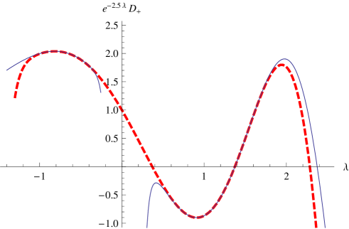
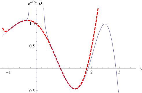
Figure 1: Plots of small- and large-$\lambda$ expansions of ${\rm e}^{-2.5\lambda}\,D_{+}$. The $\lambda$-expansion, with terms up to $\propto\lambda^{14}$ in (4.36), is shown as the dashed line. The solid lines represent the large-$\lambda$ expansions, i.e. (4.16) at negative $\lambda$, and (4.23) at positive $\lambda$; in both cases terms up to $\propto\lambda^{-6}$ are included.

Figure 2: Same as in Fig. 1, but for ${\rm e}^{-2.5\lambda}\,D_{-}$. In this case the small-$\lambda$ expansions is truncated to terms $\propto\lambda^{13}$.

Another piece of evidence supporting (4.22) is numerical. First of all, the numerical values of $\lambda_{2m}$ and $\lambda_{2m+1}$ obtained from (4.27) and (4.28), with some reasonable number of terms in the $\lambda^{-1}$ expansions included, provide remarkably accurate estimates for the eigenvalues, even for low levels. We discuss these numerics in the next section. But one can also match the large-$\lambda$ expansions of the spectral determinants to the power series expansions

$$D_{\pm}(\lambda)=1+(1\mp 1)\lambda+\sum_{s=2}^{\infty}\,D_{\pm}^{(s)}\ \lambda^{s}\,.$$ (4.36)

The latter converge in the whole $\lambda$ plane. With many terms included, the expansions (4.36) are expected to approximate the functions $D_{\pm}(\lambda)$ well even if $|\lambda|$ is not small. Since we know as many as 13 terms of (4.36), one expects to have substantial domain at negative $\lambda$ where the truncated series (4.36) match the asymptotic expansions (4.16) (again, with a reasonable number of terms in the sum). More crucially, if (4.22) is correct, there must be substantial domain of positive $\lambda$ where it matches (4.22). This comparison requires knowing the constants $d_{\pm}$ in Eqs.(4.16), (4.22). We use here the numerical estimates from the next section (see Eq. (5.1)). In Figs.2, 2 we present simultaneous plots of the $\lambda$ expansions (4.36), with as many terms as are available, and the large-$\lambda$ expansions (4.16) and (4.23), with the sums including all terms up to $\propto\lambda^{-6}$. In fact, the plots are for ${\rm e}^{-2.5\,\lambda}\,D_{\pm}(\lambda)$, with the exponential factor added to make interesting parts of all three plots visible in the same picture ($D_{\pm}(\lambda)$ themselves develop large amplitudes already at $\lambda\sim 1$). As expected, there is a good match at negative $\lambda$ between $-1$ and $-0.4$, but one can also see a clear match at positive $\lambda$, in the domain between $0.6$ and $1.6$ where the functions already show “live” behavior. Note that the two lowest zeros of both $D_{+}$ and $D_{-}$ are already visible at these orders of the $\lambda$-expansions. In fact, the positions of the lowest zeros $\lambda_{0}$ and $\lambda_{1}$ stabilize rather fast as one adds more and more terms to (4.36). This convergence is particularly impressive for $\lambda_{0}$. Pad${\acute{\rm e}}$ approximation of the $\lambda$-expansion of the ratio ${D_{+}(\lambda)\over D_{-}(\lambda)}$, Eq.(2.20), yields the following estimate of the lowest eigenvalue,

$$2\lambda_{0}=0.737061746292690\ .$$ (4.37)

Compare this number to the numerical result in Table 1.

5 Numerical results

As was mentioned, it is not difficult to compute eigenvalues $\{\lambda_{n}\}$ by direct numerical solution of equation (1.1). A variety of numerical methods exists [1, 2, 3, 4, 5]. We have used the expansion of $\varphi(x)$ in Chebyshev polynomials from [2, 4], which seems particularly suitable in the case (1.5) since it automatically guarantees the function $\varphi(x)$ correct behavior near the boundaries $x=0,1$ (besides, its implementation requires perhaps the least amount of creative programming). With this method, fourteen significant digits for as many as 50 lowest eigenvalues $\lambda_{n}$ can be obtained by truncating to matrices of the size $400\times 400$. Below we use the notation $\lambda_{n}^{\text{(num)}}$ for these numerical estimates.

$n$	$2\lambda_{n}$ from Eq. (1.6)	$2\lambda_{n}^{(7)}$	$2\,\delta\lambda_{n}^{(7)}$	$2\lambda_{n}^{(\text{num})}$
$0$	0.730	******	******	0.73706174629269
$2$	2.748145	2.748159	$6.3\times 10^{-5}$	2.7481609123706
$4$	4.749299	4.7492955	$1.8\times 10^{-6}$	4.7492953810375
$6$	6.749631	6.74962943	$1.7\times 10^{-7}$	6.7496294196488
$8$	8.7497729	8.749771584	$2.9\times 10^{-8}$	8.7497715807892
$10$	10.7498458	10.7498450900	$6.7\times 10^{-9}$	10.749845089160
$12$	12.7498885	12.7498880086	$2.0\times 10^{-9}$	12.749888008416
$14$	14.7499156	14.74991524453	$6.9\times 10^{-10}$	14.749915244446
$16$	16.7499338	16.74993361109	$2.7\times 10^{-10}$	16.749933611057
$18$	18.74994673	18.74994658405	$1.2\times 10^{-10}$	18.749946584034
$20$	20.74995619	20.749956088181	$5.4\times 10^{-11}$	20.749956088173
$22$	22.74996334	22.749963259765	$2.7\times 10^{-11}$	22.749963259761
$24$	24.74996886	24.749968804885	$1.4\times 10^{-11}$	24.749968804883
$26$	26.74997323	26.749973181147	$7.5\times 10^{-12}$	26.749973181145
$28$	28.74997673	28.749976695732	$4.2\times 10^{-12}$	28.749976695731

Table 1: Numerical values of the even eigenvalues $2\lambda_{n}$ from the large-$\lambda$ expansion. The first column gives simply the numerical values of (1.6), with all higher corrections ignored. $2\lambda_{n}^{(7)}$ are obtained from (4.27) with the sum truncated beyond the term $\propto\lambda^{-7}$. The differences $2\delta\lambda_{n}^{(7)}=2\lambda_{n}^{(7)}-2\lambda_{n}^{(6)}$ are given in the third column, they show the effect of the term $\propto\lambda^{-7}$. In the last column we present the eigenvalues $2\lambda_{n}^{(\text{num})}$ computed by direct numerical solution of (1.1).

$n$	$2\lambda_{n}$ from Eq. (1.6)	$2\lambda_{n}^{(7)}$	$2\,\delta\lambda_{n}^{(7)}$	$2\lambda_{n}^{(\text{num})}$
$1$	1.75381	1.75396	$-9.3\times 10^{-4}$	1.7537313369175
$3$	3.751045	3.7510570	$-8.6\times 10^{-6}$	3.7510575817054
$5$	5.750487	5.75049257	$-5.0\times 10^{-7}$	5.7504926236487
$7$	7.7502819	7.750284389	$-6.4\times 10^{-8}$	7.7502843971925
$9$	9.7501838	9.750185133	$-1.3\times 10^{-8}$	9.7501851352539
$11$	11.7501294	11.7501301421	$-3.4\times 10^{-9}$	11.750130142515
$13$	13.7500960	13.7500965038	$-1.1\times 10^{-9}$	13.750096503972
$15$	15.7500741	15.75007442838	$-4.0\times 10^{-10}$	15.750074428438
$17$	17.7500589	17.75005915901	$-1.6\times 10^{-10}$	17.750059159035
$19$	19.75004800	19.750048157159	$-7.2\times 10^{-11}$	19.750048157169
$21$	21.75003985	21.750039967124	$-3.4\times 10^{-11}$	21.750039967130
$23$	23.75003362	23.750033705315	$-1.7\times 10^{-11}$	23.750033705317
$25$	25.75002874	25.750028810058	$-9.0\times 10^{-12}$	25.750028810060
$27$	27.75002486	27.750024910393	$-4.9\times 10^{-12}$	27.750024910394
$29$	29.75002171	29.750021753287	$-2.7\times 10^{-12}$	29.750021753287

Table 2: The same as in Table 1, but for the odd eigenvalues $2\lambda_{n}$.

In Tables 1 and 2 we compare these numbers, for even and odd $n$ separately, with the results of large-$\lambda$ expansions. The first column in each of these tables shows numerical values yielded by Eq.(1.6), with all terms explicitly written there included. One can observe significant improvement as compared to the leading semiclassical approximation $\lambda_{n}\approx n+{3\over 4}$, even for the low levels such as $\lambda_{1}$ and $\lambda_{2}$. The approximation (1.6) corresponds to truncating the sums in Eq.(4.27) and (4.28) to terms $\sim\lambda^{-3}$, but one can obtain further corrections by including higher-order terms. We denote $\lambda_{n}^{(k)}$ the estimates from equations (4.27), (4.28) with terms up to $\propto\lambda^{-k}$ included, and present the numerical values of $\lambda_{n}^{(7)}$ (together with the deviations $\delta\lambda^{(7)}_{n}=\lambda_{n}^{(7)}-\lambda_{n}^{(6)}$ to show the expected accuracy of this approximation). Since we are dealing with an asymptotic expansion, one does not expect it to work well for low levels, but Tables 1, 2 show that including these further corrections results in noticeable improvement even for levels as low as $\lambda_{3}$ and $\lambda_{4}$, and for higher levels the improvement becomes impressive. For $n\geq 30$ $\lambda_{n}^{(7)}$ are indistinguishable from $\lambda_{n}^{\rm(num)}$ within the accuracy of the latter.

Another impressive agreement is in terms of the sum rules (1.7), (4.18). One can evaluate the spectral sums in (1.7), (4.18) using the numerical values $\lambda_{n}^{(\text{num})}$, and compare these numerical estimates $\big{[}\,G_{\pm}^{(s)}\,\big{]}^{(\rm num)}$ with the analytic predictions (1), (4.19) and (7), (7). In fact, for low $s$ the sums do not converge that fast. For instance, to estimate $\big{[}\,G_{\pm}^{(2)}\,\big{]}^{(\rm num)}$ to fourteen digits one needs to include as many as $10^{7}$ eigenvalues. Of course, this problem is easy to solve since we have very good large-$n$ asymptotic approximations. In the sums (1.7), starting from some sufficiently large $n$ one simply replaces $\lambda_{n}^{(\text{num})}$ by the asymptotic form, say $\lambda_{n}^{(7)}$. In Table 3 we show numerical estimates obtained in this way for $s=1,2,\ldots,8$. It is an easy and pleasant exercise to check that these numbers agree with the analytic expressions (1), (4.19) and (7), (7) to all digits presented. As was mentioned, we actually have analytic expressions for $G_{\pm}^{(s)}$ with $s$ up to 13, and we have verified similar agreement for these higher values of $s$ as well.

$s$	$\big{[}\,G_{+}^{(s)}\,\big{]}^{(\rm num)}$	$\big{[}\,G_{-}^{(s)}\,\big{]}^{(\rm num)}$
$1$	2.22417142752923	0.2241714275292
$2$	8.4143983221171	2.0000000000000
$3$	20.4981207536828	1.7198241782619
$4$	54.538349992708	1.7952480377615
$5$	147.32680373214	1.9789889429098
$6$	399.32397653715	2.2250507748184
$7$	1083.2464075913	2.521777906136
$8$	2939.1433918727	2.867885373267

Table 3: Numerical values of of the spectral sums (1.7), (4.18).

We also have computed the products (4.21) with the numerical spectrum,

$$d_{+}^{(\text{num})}=0.963178456398\,,\ \ \qquad d_{-}^{(\text{num})}=0.433582639833\,.$$ (5.1)

Again, it is easy to check that these numbers comply with (4.20) to twelve digits.

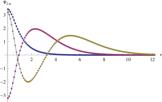
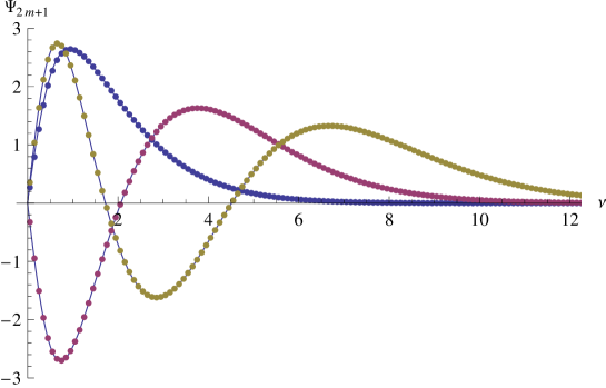
Figure 3: Comparison of the approximation (5.2) for for even eigenfuctions ${\Psi}_{n}(\nu)$ with $n=0,\,2,\,4$ (solid lines) with the results of direct numerical solution of (2.2) (bullets).

Figure 4: Comparison of the approximation (5.2) for for odd eigenfuctions ${\Psi}_{n}(\nu)$ with $n=1,\,3,\,5$ (solid lines) with the results of direct numerical solution of (2.2) (bullets).

The above numerics concern the eigenvalues $\{\lambda_{n}\}$. But it is also interesting to see how the large-$\lambda$ expansions in Section 4 approximate the associated eigenfunctions $\Psi_{n}(\nu)$. It turns out that (4.9) provides a rather good approximation even if one retains only the leading term 1 in the expansion (4.10) of the coefficients $R_{\pm}(z,\lambda)$. In this approximation the sum in (4.7) is understood as the hypergeometric function $(-{\rm i}z)^{1+\frac{{\rm i}\nu}{2}}\,U(1+\frac{{\rm i}\nu}{2},2,-{\rm i}z)$. This results in the following approximate expression for the normalized eigenfunctions (which we write for $\nu>0$; the $\nu<0$ part is restored by symmetry),

$${\Psi}_{n}(\nu)\approx{\sqrt{8}\,\pi\lambda_{n}\ \sinh^{2}({\pi\nu\over 2})\over\cosh({\pi\nu\over 2})\sqrt{1+{\rm e}^{-\pi\nu}}}\ \ \Re e\bigg{[}\,{\rm i}^{n}\ {\rm e}^{-{\rm i}\Phi(\nu)}\ \Gamma\big{(}{\textstyle{i\nu\over 2}}\big{)}\ U\Big{(}1+{\textstyle{{\rm i}\nu\over 2}},\,2,\,-2{\rm i}\pi\lambda_{n}\tanh\big{(}{\textstyle{\pi\nu\over 2}}\big{)}\,\Big{)}\,\bigg{]}\,.$$ (5.2)

Here the phase $\Phi(\nu)$ has expression

$$\Phi(\nu)={\rm sgn}(\nu)\ \bigg{[}\,{\pi\over 8}-{1\over 4\pi}\ {\rm e}^{-\pi|\nu|}\ \Phi\big{(}{\rm e}^{-2\pi|\nu|},\,2,\,{\textstyle{1\over 2}}\,\big{)}\ \bigg{]}\ ,$$ (5.3)

in terms of the Lerch transcendent $\Phi(z,s,a)=\sum_{k=0}^{\infty}{z^{k}\over(k+a)^{s}}$. The approximation is not expected to be very accurate at small $\nu$, because (5.2) has a term with singularity $\sim\nu\,\log\nu$ at $\nu=0$, while true eigenfunctions $\Psi_{n}(\nu)$ are analytic at all real $\nu$ (recall that the higher order terms in (4.10) were designed precisely to fix this analytic deficiency). However, numerically the deviations of (5.2) from true eigenfunctions are rather small even at small $\nu$. Figs. 4, 4 show plots of (5.2) for low $n$ against the corresponding eigenfunctions obtained by numerical solution of (2.2). Deviation at small $\nu$ is barely visible only for $n=0$.

6 Remarks

As was mentioned in the introduction, the techniques developed here extend to the case (1.9). While we plan to treat this case in a separate paper, let us announce here some preliminary results. The large-$\lambda$ expansion generalizes in an almost straightforward way, yielding the asymptotic large-$n$ expansion of $\lambda_{n}(\alpha)$. The large-$n$ behavior follows from the “quantization condition”, generalizing (4.27), (4.28) in Section 4,

$$2\lambda - {2\alpha\over\pi^{2}}\ \log(2\lambda)-C_{0}(\alpha)+{\alpha^{2}\over\pi^{4}\lambda}+{1\over 2\pi^{6}\ \lambda^{2}}\,\Big{[}\,\alpha^{3}+(-1)^{n}\,\pi^{2}\,(1+\alpha)\,\Big{]}$$ (6.1)

$$+ {1\over 12\pi^{8}\,\lambda^{3}}\,\Big{[}\,5\alpha^{4}+\pi^{2}\,(1+\alpha)^{2}-(-1)^{n}\,12\pi^{2}\,(1+\alpha)\,\big{(}\log\big{(}2\pi{\rm e}^{\gamma_{E}}\lambda\big{)}-C_{1}(\alpha)\big{)}\,\Big{]}$$

$$+ O\big{(}\lambda^{-4}\log^{2}(\lambda)\big{)}=n\,,$$

where

$$C_{0}(\alpha) = {3\over 4}+{2\alpha\over\pi^{2}}\ \log\big{(}4\pi{\rm e}^{\gamma_{E}}\big{)}-{\alpha^{2}\over 2\pi^{2}}\int_{-\infty}^{\infty}{\rm d}t\,{\sinh(t)\,(\,\sinh(2t)-2t)\over t\,\cosh^{2}(t)\,\big{(}\,\alpha\,\sinh(t)+t\,\cosh(t)\,\big{)}}\,,$$ (6.2)

$$C_{1}(\alpha) = \frac{1}{2}+\frac{3\alpha}{2}+{\alpha\over 8}\ \int_{-\infty}^{\infty}{\rm d}t\ \ {\sinh(2t)-2t\over t\,\sinh(t)\,\big{(}\,\alpha\,\sinh(t)+t\,\cosh(t)\,\big{)}}\ .$$

The first two terms in (6.1) are known since [1]. Explicit expression for the constant term $C_{0}(\alpha)$, Eq.(6.2), was previously obtained in [11] (see also [12]). We believe the higher order terms in the expansion in (6.1) are new. Further terms can be derived in a systematic way. Another result compact enough to be presented here is the analytic expression of the spectral sums (4.19),

$$G_{\pm}^{(1)}(\alpha)=\log(8\pi)-2\pm 1-{\alpha\over 4}\ \int_{-\infty}^{\infty}{\rm d}t\ {\sinh(t)\ (\sinh(2t)\pm 2t)\over t\,\cosh^{2}(t)\,(\alpha\sinh(t)+t\,\cosh(t)\,)}\ .$$ (6.3)

These and other results indicate the rich analytic structure of $\lambda_{n}(\alpha)$ as the functions of complex $\alpha$. First, as expected, $\lambda_{n}(\alpha)$ have square-root branching point $\alpha=-1$, which corresponds to the limit $m_{1}=m_{2}=0$, where the chiral symmetry becomes exact. In particular, the lowest eigenvalue $\lambda_{0}(\alpha)$ turns to zero as $\sqrt{\alpha+1}$. But in addition, there are infinitely many similar square-root branching points located on the second sheet of the $\alpha$-plane (i.e. in the left half plane of the variable $\sqrt{\alpha+1}$), accumulating towards $\alpha=\infty$. At each of these points one of the even eigenvalues $\lambda_{2m}(\alpha)$ turns to zero. It is difficult to imagine that if one takes QCD₂ with large but finite $N_{c}$ these singularities just disappear. It is more likely that they become nontrivial critical points of some sort. What are the physics of these critical points? Can one identify associated (nonunitary) CFT? These are some of intriguing questions which we plan to study in the future.

7 Appendix A

A1. Analytic expressions for the spectral sums (1.7) with $s=2,\,3,\,4$ are given in (1). Here we present few more expressions for $G_{\pm}^{(s)}$, with $s$ up to 8:

$$G^{(5)}_{+}=\frac{2}{135}\big{[}\,16\pi^{4}-50\pi^{2}(2+21\zeta(3))+105\left(20\zeta(3)+105\zeta^{2}(3)+31\zeta(5)\right)\,\big{]}$$

$$G^{(6)}_{+}=\frac{1}{4320}\,\big{[}\,\pi^{4}(4090+1449\zeta(3))-20\pi^{2}\left(140+9912\zeta(3)+2646\zeta(3)^{2}+837\zeta(5)\right)$$

$$+15\left(138768\zeta^{2}(3)+24696\zeta^{3}(3)+16120\zeta(5)+28\zeta(3)(140+837\zeta(5))+3429\zeta(7)\right)\,\big{]}$$

$$G^{(7)}_{+}=\frac{1}{567000}\,\big{[}\,-12288\pi^{6}+49\pi^{4}(21002+45969\zeta(3))-2940\pi^{2}\big{(}36+15400\zeta(3)$$

$$+22050\zeta^{2}(3)+4495\zeta(5)\big{)}+315\big{(}1509200\zeta^{2}(3)+1440600\zeta^{3}(3)+60760\zeta(5)$$

$$+196\zeta(3)(36+4495\zeta(5))+51689\zeta(7)\big{)}\,\big{]}$$ (7.1)

$$G^{(8)}_{+}=\frac{1}{1944000}\,\big{[}\,-4\pi^{6}(97286+12375\zeta(3))+\pi^{4}\big{(}4210624+38551128\zeta(3)$$

$$+5622750\zeta^{2}(3)+767250\zeta(5)\big{)}-30\pi^{2}\big{(}2464+32104800\zeta^{2}(3)+3704400\zeta^{3}(3)$$

$$+4032480\zeta(5)+8400\zeta(3)(712+279\zeta(5))+142875\zeta(7)\big{)}+315\big{(}21403200\zeta^{3}(3)$$

$$+1852200\zeta^{4}(3)+76880\zeta(5)+432450\zeta^{2}(5)+8400\zeta^{2}(3)(712+279\zeta(5))$$

$$+167132\zeta(7)+\zeta(3)(4928+8064960\zeta(5)+285750\zeta(7))+27375\zeta(9)\big{)}\,\big{]}$$

$$G^{(5)}_{-}=\frac{1}{225}\big{[}\,-32\pi^{4}+50\pi^{2}(6+7\zeta(3))-15(76+155\zeta(5))\,\big{]}$$

$$G^{(6)}_{-}=\frac{1}{97200}\,\big{[}\,681120-214800\pi^{2}+14426\pi^{4}+201600\pi^{2}\zeta(3)-21735\pi^{4}\zeta(3)$$

$$-1339200\zeta(5)+251100\pi^{2}\zeta(5)-771525\zeta(7)\,\big{]}$$

$$G^{(7)}_{-}=\frac{1}{1190700}\,\big{[}\,-11541600+4245360\pi^{2}-519302\pi^{4}+18432\pi^{6}$$

$$+21609\pi^{4}\zeta(3)+1367100\pi^{2}\zeta(5)-10921365\zeta(7)\,\big{]}$$ (7.2)

$$G^{(8)}_{-}=\frac{1}{76204800}\,\big{[}\,1021799520-429522240\pi^{2}+60393480\pi^{4}-2819800\pi^{6}$$

$$+110308800\pi^{2}\zeta(3)-34223168\pi^{4}\zeta(3)+1455300\pi^{6}\zeta(3)+25930800\pi^{4}\zeta^{2}(3)$$

$$-732765600\zeta(5)+346332000\pi^{2}\zeta(5)-22557150\pi^{4}\zeta(5)-344509200\pi^{2}\zeta(3)\zeta(5)$$

$$+1144262700\zeta^{2}(5)-860267520\zeta(7)+126015750\pi^{2}\zeta(7)-253519875\zeta(9)\,\big{]}$$

Expressions for $G_{\pm}^{(s)}$ with even higher $s$ (we have them all the way up to $s=13$) have similar structure, but appear too cumbersome to fit in reasonable page space.

A2. Coefficients $\Phi_{\pm}^{(k)}(l)$ in Eqs.(4.27), (4.28) for $k\leq 7$:

$$\Phi_{+}^{(2)}(l) = -\frac{1}{2\pi^{4}}$$

$$\Phi_{+}^{(3)}(l) = \frac{12\,l-7}{12\pi^{6}}$$

$$\Phi_{+}^{(4)}(l) = \frac{1}{16\pi^{8}}\ \Big{[}\,16\pi^{2}-5+44\,l-24\,l^{2}\,\Big{]}$$

$$\Phi_{+}^{(5)}(l) = \frac{1}{12\pi^{10}}\ \Big{[}\,3+76\pi^{2}+12\zeta(3)+(48-60\pi^{2})\,l-84\,l^{2}+24\,l^{3}\,\Big{]}$$

$$\Phi_{+}^{(6)}(l) = \frac{1}{144\pi^{12}}\ \Big{[}\,111+2965\pi^{2}-828\pi^{4}+948\zeta(3)+\big{(}\,396-6228\pi^{2}-720\zeta(3)\,\big{)}\,l$$ (7.3)

$$+ (2160\pi^{2}-2448)\,l^{2}+1968\,l^{3}-360\,l^{4}\,\Big{]}$$

$$\Phi_{+}^{(7)}(l) = \frac{1}{960\pi^{14}}\ \Big{[}\,870+40865\pi^{2}-79264\pi^{4}+21560\zeta(3)-16800\pi^{2}\zeta(3)+4320\zeta(5)$$

$$- \big{(}1800+181680\pi^{2}-47040\pi^{4}+42720\zeta(3)\big{)}\,l+\big{(}160320\pi^{2}-24240$$

$$+ 14400\zeta(3)\,\big{)}\,l^{2}+(45760-33600\pi^{2})\,l^{3}-22080\,l^{4}+2880\,l^{5}\,\Big{]}\ .$$

$$\Phi_{-}^{(2)}(l) = \frac{1}{2\pi^{4}}$$

$$\Phi_{-}^{(3)}(l) = \frac{5-12\,l}{12\pi^{6}}$$

$$\Phi_{-}^{(4)}(l) = \frac{1}{16\pi^{8}}\ \Big{[}\,3-16\pi^{2}-36\,l+24\,l^{2}\,\Big{]}$$

$$\Phi_{-}^{(5)}(l) = \frac{1}{12\pi^{10}}\ \Big{[}\,-3-70\pi^{2}-12\zeta(3)+(60\pi^{2}-36)\,l+72\,l^{2}-24\,l^{3}\,\Big{]}$$

$$\Phi_{-}^{(6)}(l) = \frac{1}{144\pi^{12}}\ \Big{[}\,828\pi^{4}-87-2633\pi^{2}-900\zeta(3)+\big{(}\,5820\pi^{2}-252+720\zeta(3)\,\big{)}\,l$$ (7.4)

$$+ (1944-2160\pi^{2})\,l^{2}-1728\,l^{3}+360\,l^{4}\,\Big{]}$$

$$\Phi_{-}^{(7)}(l) = \frac{1}{960\pi^{14}}\ \Big{[}\,76864\pi^{4}-630-35355\pi^{2}-19800\zeta(3)+16800\pi^{2}\zeta(3)-4320\zeta(5)$$

$$+ \big{(}1800+163920\pi^{2}-47040\pi^{4}+40800\zeta(3)\,\big{)}\,l+\big{(}\,18000-151200\pi^{2}$$

$$- 14400\zeta(3)\,\big{)}\,l^{2}+(33600\pi^{2}-37440)\,l^{3}+19680\,l^{4}-2880\,l^{5}\,\Big{]}\ .$$

8 Appendix B

Here we describe some technical details of our analysis of the integral equation (2.8) with the r.h.s. (2.11). To make the equations shorter, throughout this appendix we trade the variable $\nu$ for

$$t\equiv{\pi\nu\over 2}\ ,$$ (8.1)

but, with some abuse of notations, retain the same symbols for basic functions. Thus $\Psi_{\pm}(t|\lambda)$ will stand for solutions of the integral equations

$$f(t)\,\Psi_{+}(t|\lambda)-{t\over\sinh(t)} = \lambda\ \int_{-\infty}^{\infty}{\rm d}t^{\prime}\ S(t-t^{\prime})\ \Psi_{+}(t^{\prime}|\lambda)$$ (8.2)

$$f(t)\,\Psi_{-}(t|\lambda)-{\pi\over 2\sinh(t)} = \lambda\ \mathchoice{{\vbox{\hbox{$\textstyle-$}}\kern-4.86108pt}}{{\vbox{\hbox{$\scriptstyle-$}}\kern-3.25pt}}{{\vbox{\hbox{$\scriptscriptstyle-$}}\kern-2.29166pt}}{{\vbox{\hbox{$\scriptscriptstyle-$}}\kern-1.875pt}}\!\int_{-\infty}^{\infty}{\rm d}t^{\prime}\ S(t-t^{\prime})\ \Psi_{-}(t^{\prime}|\lambda)\ ,$$

with the kernel

$$S(t)={t\over\sinh(t)}\ .$$ (8.3)

The analysis below does not depend on a specific form of the function $f(t)$. With $f(t)=t\,\coth(t)$, Eqs.(8.2) are equivalent to (2.8), (2.11), but almost all statements below remain valid if one takes the more general form

$$f(t)=\alpha+t\,\coth(t)\ ,$$ (8.4)

which appears in analysis of (1.1) with nonzero but equal $\alpha_{1}=\alpha_{2}=\alpha$.

Eq.(8.2) defines the spectral problem

$${\hat{K}}\,\phi(t)=\lambda^{-1}\ \phi(t)$$ (8.5)

for the Fredholm operator

$${\hat{K}}\phi(t)\equiv\int_{-\infty}^{\infty}{\rm d}t^{\prime}\,K(t,t^{\prime})\ \phi(t^{\prime})$$ (8.6)

with the kernel

$$K(t,t^{\prime})={S(t-t^{\prime})\over\sqrt{f(t)f(t^{\prime})}}\ ,$$ (8.7)

where $\phi=\sqrt{f}\ \Psi$. Let $R(t,t^{\prime}|\lambda)$ be the corresponding resolvent, i.e. the kernel of the operator ${{\hat{K}}\over 1-\lambda{\hat{K}}}$. By definition, it satisfies the equation

$$R(t,t^{\prime}|\lambda)-\lambda\ \int_{-\infty}^{\infty}{\rm d}\tau\ K(t,\tau)\ R(\tau,t^{\prime}|\lambda)=K(t,t^{\prime})\ .$$ (8.8)

The spectral sums (1.7) and (4.18) are related to the resolvent by the trace identities

$$\sum_{s=1}^{\infty}\big{[}\,G_{+}^{(s)}+G_{-}^{(s)}\,\big{]}\ \lambda^{s-1} = {\rm C}+\int_{-\infty}^{\infty}{\rm d}t\ \big{[}\,R(t,t|\lambda)-R^{(0)}(t)\,\big{]}$$ (8.9)

$$\sum_{s=1}^{\infty}\big{[}\,G_{+}^{(s)}-G_{-}^{(s)}\,\big{]}\ \lambda^{s-1} = \int_{-\infty}^{\infty}{\rm d}t\ R(t,-t|\lambda)\ .$$ (8.10)

The constant C in (8.9) depends on the choice of the subtraction term $R^{(0)}(t)$ needed to make the integral convergent. We take

$$R^{(0)}(t)=\frac{\tanh(t)}{t}\ .$$ (8.11)

With this choice the constant can be shown to be exactly

$${\rm C}=2\,\log(8\pi)-4\ .$$ (8.12)

It is the remarkable property of the kernel (8.3) in (8.2) that the resolvent can be expressed in a simple way through the functions $\Psi_{+}(t|\lambda)$ and $\Psi_{-}(t|\lambda)$, namely

$$R(t,t^{\prime}|\lambda)={2\sinh(t)\sinh(t^{\prime})\over\pi\,\sinh(t^{\prime}-t)}\ \sqrt{f(t)f(t^{\prime})}\ \Big{[}\,\Psi_{+}(t^{\prime}|\lambda)\Psi_{-}(t|\lambda)-\Psi_{-}(t^{\prime}|\lambda)\Psi_{+}(t|\lambda)\,\Big{]}\ .$$ (8.13)

To prove this identity, consider the Liouville - Neumann series for $\Psi_{\pm}(t|\lambda)$,

$$f(t)\,\Psi_{+}(t|\lambda) = \sum_{k=0}^{\infty}\lambda^{k}\ \int_{-\infty}^{\infty}{t_{k}\over\sinh(t_{k})}\ \prod_{j=1}^{k}{{\rm d}t_{j}\over f(t_{j})}\ S(t_{j}-t_{j-1})$$ (8.14)

$$f(t)\,\Psi_{-}(t|\lambda) = {{\pi\over 2}}\ \sum_{k=0}^{\infty}\lambda^{k}\ \mathchoice{{\vbox{\hbox{$\textstyle-$}}\kern-4.86108pt}}{{\vbox{\hbox{$\scriptstyle-$}}\kern-3.25pt}}{{\vbox{\hbox{$\scriptscriptstyle-$}}\kern-2.29166pt}}{{\vbox{\hbox{$\scriptscriptstyle-$}}\kern-1.875pt}}\!\int_{-\infty}^{\infty}{1\over\sinh(t_{k})}\prod_{j=1}^{k}{{\rm d}t_{j}\over f(t_{j})}\ S(t_{j}-t_{j-1})\ ,$$

where $t_{0}\equiv t$. Then we have

$${\textstyle{2\over\pi}}\ f(t)f(t^{\prime})\Big{[}\,\Psi_{+}({t^{\prime}}|\lambda)\Psi_{-}(t|\lambda)-\Psi_{-}({t^{\prime}}|\lambda)\Psi_{+}(t|\lambda)\,\Big{]}=\sum_{k,m}\lambda^{k+m}\mathchoice{{\vbox{\hbox{$\textstyle-$}}\kern-4.86108pt}}{{\vbox{\hbox{$\scriptstyle-$}}\kern-3.25pt}}{{\vbox{\hbox{$\scriptscriptstyle-$}}\kern-2.29166pt}}{{\vbox{\hbox{$\scriptscriptstyle-$}}\kern-1.875pt}}\!\int_{-\infty}^{\infty}\ {\sinh(t^{\prime}_{k}-t_{m})\over\sinh(t^{\prime}_{k})\sinh(t_{m})}\times$$

$$\ \ \ \ S(t^{\prime}_{k}-t_{m})\ \prod_{j=1}^{k}{{\rm d}t^{\prime}_{j}\over f(t^{\prime}_{j})}\ S(t^{\prime}_{j}-t^{\prime}_{j-1})\ \ \prod_{i=1}^{m}{{\rm d}t_{i}\over f(t_{i})}\ S(t_{i}-t_{i-1})\ ,$$ (8.15)

where again $t_{0}=t$ and $t_{0}^{\prime}=t^{\prime}$. Let us introduce uniform notations for the integration variables

$$(t_{1},\ldots t_{m};t^{\prime}_{k},\ldots t^{\prime}_{1})=(\tau_{1},\ldots\tau_{m},\tau_{m+1},\ldots\tau_{k+m})\ .$$ (8.16)

The elementary identity

$$\sum_{m=0}^{l}{\sinh(\tau_{m+1}-\tau_{m})\over\sinh(\tau_{m+1})\sinh(\tau_{m})}={\sinh(\tau_{l+1}-\tau_{0})\over\sin(\tau_{l+1})\sinh(\tau_{0})}\ ,$$ (8.17)

allows one to put (8) in compact form

$${2\sinh(t)\sinh(t^{\prime})\over\pi\,\sinh(t^{\prime}-t)}\ f(t)f(t^{\prime})\,\big{[}\,\Psi_{+}(t^{\prime}|\lambda)\Psi_{-}(t|\lambda)-\Psi_{-}(t^{\prime}|\lambda)\Psi_{+}(t|\lambda)\,\big{]}=$$

$$\ \ \ \ \ \ \ \ \ \ \ \ \ \ \ \ \ \ \ \ \ \ \ \ \sum_{l=1}^{\infty}\lambda^{l}\int_{-\infty}^{\infty}\prod_{j=1}^{l}{{\rm d}\tau_{j}\over f(\tau_{j})}\ \prod_{j=1}^{l+1}S(\tau_{j}-\tau_{j-1})\ ,$$ (8.18)

where now $\tau_{0}\equiv t$, $\tau_{l+1}=t^{\prime}$. It is easy to see that the right-hand side here divided by $\sqrt{f(t)f(t^{\prime})}$ is exactly the Liouville - Neumann series for the solution of the integral equation (8.8).

Now, since

$$D_{\pm}(\lambda)=\Big{(}{8\pi\over{\rm e}}\Big{)}^{\lambda}\ \exp\bigg{[}-\sum_{s=1}^{\infty}s^{-1}\ G_{\pm}^{(s)}\ \lambda^{s}\,\bigg{]}\ ,$$ (8.19)

combining Eqs.(8.9), (8.10) and (8.13) leads to the following expressions for the logarithmic derivatives of the spectral determinants,

$$\partial_{\lambda}\log(D_{+}D_{-})=2-\qquad\qquad$$ (8.20)

$$\ \ \ \int_{-\infty}^{\infty}{\rm d}t\ \bigg{\{}\,{\pi\over 2f(t)}\ \ \Big{[}\,Q_{-}(t|\lambda)\partial_{t}Q_{+}(t|\lambda)-Q_{+}(t|\lambda)\partial_{t}Q_{-}(t|\lambda)\,\Big{]}-\frac{\tanh(t)}{t}\,\bigg{\}}$$

$$\partial_{\lambda}\log\Big{(}{D_{+}\over D_{-}}\Big{)}=-\int_{-\infty}^{\infty}{{\rm d}t\over f(t)}\ \ \ {\pi\,Q_{+}(t|\lambda)Q_{-}(t|\lambda)\over\sinh(2t)}\ ,$$

where

$$Q_{\pm}(t|\lambda)={\textstyle{2\over\pi}}\ \sinh(t)\ f(t)\ \Psi_{\pm}(t|\lambda)\ .$$ (8.21)

The above analysis, in particular Eqs.(8.20), applies to (8.2) with generic $f(t)$. If one takes $f(t)$ of the special form $t\,\coth(t)$, it is very likely that (8.20) further reduce to the simple form (2.17). Note that (2.17) corresponds to replacing the integrals in (8.20), (8.20) by one half of the residues of the integrands at the pole at $t={{\rm i}\pi\over 2}$. Unfortunately, so far we could not find a way to reduce the integrals to the residues, and thus (2.17) lacks rigorous proof. But it passes a number of nontrivial tests, both analytic and numerical. Thus, all $G_{\pm}^{(s)}$ listed in (1) come out identical by direct evaluation of the integrals from (8.20). For higher $s$, using (2.17) instead of (8.20) dramatically simplifies calculations, and all analytic expressions for $G_{\pm}^{(s)}$ listed in Appendix A and beyond in fact depend on the validity of (2.17). We take agreement with the numerical data in Table 3 as further support of (2.17). On the other hand, although in deriving the large-$\lambda$ expansion of the spectrum in Section 4 we have used (2.17), it is possible to show that the results for the coefficients $\Phi_{\pm}^{(k)}(l)$ in (4.27), (4.28) are independent of the validity of this relation. In particular, all expressions for these coefficients in Appendix A can be re-derived by a different (somewhat more complicated) method which does not rely on (2.17). Let us stress also that the simplification (2.17) depends on the special choice $f(t)=t\,\coth(t)$ in (8.2). It is unlikely that any simple modification of (2.17) exists for more general $f(t)$, say of the form (8.4). Therefore, in the analysis of the problem (1.1) in the more interesting case of a generic $\alpha$ (which we plan to present in a separate paper), we have to make do with the integral representation (8.20).

References

[1] G. ’t Hooft, A Two-dimensional model for mesons,
Nucl. Phys. B75 (1974) 461-470
[2] A.J. Hanson, R.D. Peccei and M.K. Prasad,
Two-dimensional gauge theory, strings and wings:
Comparative analysis of meson spectra and covariance,
Nucl. Phys. B121 (1977) 477-504
[3]
S. Huang, J.W. Negele and J. Polonyi,
Lattice gauge theory and the structure of the vacuum and hadrons,
Nucl. Phys. B307 (1988) 669-704
[4] R.L. Jaffe and P.F. Mende, When is field theory effective?,
Nucl. Phys. B369 (1992) 189-218
[5]
W. Krauth and M. Staudacher,
Nonintegrability of two-dimensional QCD,
Phys. Lett. B388 (1996) 808-812
[6]
P. Fonseca and A. Zamolodchikov,
Ising Spectroscopy I: Mesons at ,
RUNHETC-2006-13, hep-th arXiv:0612.304
[7]
S.B. Rutkevich,
Formfactor perturbation expansions and confinement in the Ising field theory,
Preprint 2009, cond-mat arXiv:0901.1571
[8]
R. Narayanan and H. Neuberger, The quark mass dependence of the
pion mass at infinite , Phys. Lett. B616 (2005) 76-84
[9]
C.G. Callan, Jr., N. Coote and D.J. Gross, Two-dimensional
Yang-Mills theory: A model of quark confinement, Phys. Rev. D13, No.6 (1976) 1649-1669
[10]
M.B. Einhorn,
Confinement, form factors, and deep-inelastic scattering
in two-dimensional quantum chromodynamics,
Phys. Rev. D14, No.12 (1976) 3451-3471
[11]
R.C. Brower, W.L. Spence and J.H. Weis, Bound states and
asymptotic limits for quantum chromodynamics in two dimensions,
Phys. Rev. D19, No.10 (1979) 3024-3049
[12]
J. Mondejar and A. Pineda, Deep inelastic scattering and
factorization in the ’t Hooft model, Phys. Rev. D79, 085011
(2009)
[13]
M. Abramowitz and I.A. Stegun, Handbook of Mathematical Functions, Dover, New York (1965)