Transformation kinetics of alloys under non-isothermal conditions

Abstract

The overall solid-to-solid phase transformation kinetics under non-isothermal conditions has been modelled by means of a differential equation method. The method requires provisions for expressions of the fraction of the transformed phase in equilibrium condition and the relaxation time for transition as functions of temperature. The thermal history is an input to the model. We have used the method to calculate the time/temperature variation of the volume fraction of the favoured phase in the $\alpha\Leftrightarrow\beta$ transition in a zirconium alloy under heating and cooling, in agreement with experimental results. We also present a formulation that accounts for both additive and non-additive phase transformation processes. Moreover, a method based on the concept of path integral, which considers all the possible paths in thermal histories to reach the final state, is suggested.

1 Introduction

The kinetics of phase transformations in solids often involves the effects of heating and/or cooling rates. This is because first order phase transformations generally occur by concurrent nucleation and growth of the new phase and that both these mechanisms are time and temperature dependent [1, 2]. The overall phase transformation kinetics (nucleation plus growth) is represented by the fraction of transformed material in the system as a function of time and temperature $\phi=\phi(t,T)$. This attribute under isothermal conditions will results in a time-temperature-transformation (TTT) diagram, which is a complement to the phase diagram in equilibrium thermodynamics. Besides the nucleation rate and the growth rate, other factors that determine $\phi$ include the density and distribution of nucleation sites, the overlap of diffusion fields from neighbouring transformed volumes, and the collision by adjacent transformed domains [3].

A phenomenological stochastic kinetic model for the overall phase transformation under isothermal conditions was solved exactly by Kolmogorov [4] and later independently by Johnson and Mehl [5] and Avrami [6], the KJMA model. Early treatments of non-isothermal transformation kinetics are found in papers by Avrami [7] and Cahn [8]. Avrami [7] showed that for a special case where the nucleation rate is proportional to the the growth rate of the favoured phase, over a temperature range, the non-isothermal transformations can be considered as a series of isothermal reactions at every time step that can be linearly superposed to give the non-isothermal condition (additivity rule). Later, Cahn [8] argued that phase transformations that involve heterogeneous nucleation quite often obey an additivity rule. He noted that for such situations, a non-isothermal transformation can be related to an isothermal one through simple rate rules. More specifically, Cahn showed that if the transformation rate (${\rm d}\phi/{\rm d}t$) depends only on $\phi$ and temperature $T$, i.e. only on the state variables and not on the temperature path by which it had arrived to that state, then $\phi$ can be considered as an additive quantity. This situation occurs if the nucleation sites were consumed early in the reaction, i.e. site saturation occurs, and if the growth rate is a function of instantaneous temperature only.

Cahn’s additivity principle has been used by many workers for the evaluation of non-isothermal transformations in materials; e.g., austenite to ferrite+pearlite transformations in steels [9, 10, 11] and a similar kind of transformation in titanium alloys under cooling [12, 13]. A number of investigators have evaluated the applicability of the additivity rule in detail [14, 15, 16, 17, 18]. A general modular approach, which accounts for the three phase transformation mechanisms, nucleation, growth and impingement applicable to both isothermal and isochronous conditions, have been developed, discussed and applied to phase transitions in alloys [19, 20, 21]. A recent overview of numerical and analytical methods for the determination of the kinetic parameters of a phase transformation is provided in [22]. An analytical solution for non-isothermal KJMA rate equation comprising separate activation energies for nucleation and growth when the transformation occurs under continuous heating has been obtained [23]. In an integral concurrent approach, Elder et al. [24] have studied the non-isothermal glassy or amorphous metals (such as Fe-B, Cu-Zr and Mg-Zn alloys) by solving a set of coupled physically-based equations for time-dependent spatially uniform temperature field, for the nucleation and growth of single crystallite and the Kolmogorov [4] formula for $\phi$, simultaneously.

In this paper, we employ a method for calculation of the volume fraction of the new phase as a function of time and temperature during phase transformation in non-isothermal conditions. The method satisfies Cahn’s additivity rule and assumes that the system is not too far away from equilibrium. It requires the specification of the fraction of transformed phase in equilibrium as a function of temperature. The method has been used to compute the phase transformation behaviour of a zirconium alloy under both slow and rapid heating and cooling (up to $\pm 100$ Ks^-1). It is equivalent to the model for grain boundary nucleation when the nucleation rate is high and site saturation occurs early during the reaction [25]. The applicability of the method could be computations of transformation behaviour during fabrications subject to a variety of heat treatments, for example [26], or in-service material performance under extreme conditions [27]. We shall also outline a general method for treating cases for which the volume fraction of the transformed phase is thermal history dependent.

The organization of this paper is as follows. In section 2, a kinetic model for non-isothermal transformation, in differential form and in integro-differential form, is presented. The application of the differential method to the solid state phase transformation in a zirconium alloy is presented in section 3. In section 4, we discuss the appropriateness of the model both from a theoretical stance and empirical applicability. In section 5, we summarize the main results and remark on possible future directions.

2 Kinetic model

One common approach to model the kinetics of non-isothermal phase transformation is to utilize the so called additivity rule [7, 8]. The rule may be stated as follows: The temperature history (temperature vs. time) is subdivided into a number of small type steps. Then the time spent for a volume element of the material in time interval $\Delta t_{i}$ at a given temperature $T_{i}$ divided by the incubation time $t_{xi}$ at which the reaction has attained a certain fraction $x$ of completion, can represent the fraction of the total nucleation time required for formation of the new phase. When the sum of such fractions reaches unity, the transformation starts to occur. Symbolically, it is expressed as

$$\sum_{i=1}^{n}\frac{\Delta t_{i}}{t_{xi}}=1\quad\mbox{or}\quad\int_{0}^{t}\frac{{\rm d}s}{t_{x}[T(s)]}=1.$$ (1)

A suitable material parameter for tracing the progress of solid-state phase transformation is the transformed volume fraction $y$ as a function of time $t$ and temperature $T$ with the property $0\leq y\leq 1$.

Suppose the transformation is additive and the rate of transformation is only a function of the amount of transformation and temperature [8], namely

$$\frac{{\rm d}y}{{\rm d}t}=f(y,T),$$ (2)

The time it takes for a certain fraction $y_{x}$ of the new phase to be completed is

$$t_{x}=\int_{0}^{y_{x}}f(y,T)^{-1}dy,$$ (3)

Equation (2) is a sufficient condition for the additivity, since it satisfies the additivity rule (1) through equation (3).

Following [10], we consider that $y$ is not too far from its steady-state or equilibrium value $y_{s}(T)$ at a given temperature $T$, with $f(y_{s},T)=0$. Thus, the first term in a series expansion of $f$ about $y_{s}$ yields

$$\frac{{\rm d}y}{{\rm d}t}=\frac{y_{s}(T)-y}{\tau_{c}(T)},$$ (4)

where $\tau_{c}$ is a characteristic time of phase transformation and formally corresponds to $\tau_{c}=\big{(}\partial f/\partial y|_{y=y_{s}}\big{)}^{-1}$. Note that equation (4) is controlled by two external temperature-dependent functions, i.e., $\tau_{c}(T)$ and $y_{s}(T)$, with $y_{s}(T)$ being the fraction of a new phase reached at temperature $T$ after infinitely long time and $0\leq y_{s}(T)\leq 1$. Both these functions are material specific temperature-dependent quantities and can be deduced from experimental data on properties of a particular material or derived from appropriate models verified with such data. By putting $\phi\equiv y/y_{s}$ and $k(T)\equiv\tau_{c}^{-1}(T)$, we rewrite equation (4) in a reduced form

$$\frac{{\rm d}\phi}{{\rm d}t}=k(T)(1-\phi).$$ (5)

Integrating this equation gives

$$\phi(t)=1-\exp\Big{(}-\int_{t_{0}}^{t}k[T(s)]{\rm d}s\Big{)}.$$ (6)

Under non-isothermal conditions (heating/cooling), $\phi$ not only depends on $t$ and $T$ directly, but also on the way it has reached that temperature at a given point in time, see figure 1. This process may formally be described by means of a generalized Langevin-type equation. On these conditions, the temperature follows a path which may be an arbitrary function of time, and hence equation (4) needs to be solved numerically (section 3.2).

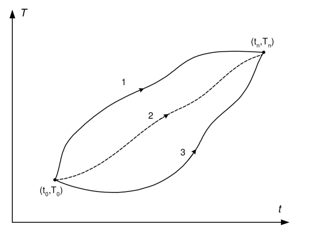
Figure 1: Time ($t$) temperature ($T$) histories. A sample undergoing a phase transformation when subjected to a thermal history from state ($t_{0},T_{0}$) to ($t_{n},T_{n}$) via different paths would reach different stages of transformations at ($t_{n},T_{n}$).

We next present a more general theoretical treatment of the kinetics of phase transformation. As pointed out in [8], if the transformation rate depends only on $y$ and $T$, i.e. on the state of the system rather on the thermal path by which it has reached that state, then the transformation is additive in the sense of equation (1). By making the ansatz $f(\phi,T)=h(T)g(\phi)$, we write equation (2) in the form

$$\frac{{\rm d}\phi}{{\rm d}t}=h(T)g(\phi).$$ (7)

As an example, for the KJMA model (A), we write

$$h(T) = mk(T)^{1-\gamma}$$ (8)

$$g(\phi) = [-\ln(1-\phi)]^{\gamma}(1-\phi),$$ (9)

with $\gamma=(m-1)/m$ and $m$ is the overall growth exponent (A). In our special case, $m=1$, thereby (7) yields equation (4).

We generalize the differential equation (7) to overcome the restriction of additivity [28]. In the manner of [29], we write

$$\frac{{\rm d}\phi}{{\rm d}t}=\int_{0}^{t}M[T(t)-T[\bar{t})]g[\phi(\bar{t})]{\rm d}\bar{t}+\eta(t),$$ (10)

where $M(t)$ is a memory kernel, which accounts for the effect of non-additivity and $\eta(t)$ is a random force, e.g. a Gaussian white noise, which stands for the thermal fluctuations of the system during phase transformation. An important property of $\eta(t)$ is that it vanishes on the average, i.e. $\langle\eta(t)\rangle=0$, and it is un-correlated to $\phi(t)$, i.e. $\langle\phi(t)\eta(t)\rangle=0$, see e.g. [30]. Also, $M(t)$ is proportional to the spectrum of the random force, viz.

$$M(t-t^{\prime})\propto\frac{1}{k_{B}T}\langle\eta(t)\eta(t^{\prime})\rangle.$$ (11)

If now $M(t)$ decays in a time $\tau_{M}$ and the applicable time is much longer than $\tau_{M}$, then

$$M(T[t]-T[\bar{t})])=h(T)\delta(t-\bar{t}),$$ (12)

where $\delta(t)$ is the Dirac delta function. Thus, with relation (12), Eq. (10) reduces to (7), that is when only the additivity rule is applicable.

Let us now consider the case of non-isothermal transformation with a path-dependent characteristic. Suppose the volume fraction transformed obeys a general relation in the form

$$\frac{{\rm D}y}{{\rm D}T}=F[\varphi(T)],$$ (13)

where ${\rm D}y/{\rm D}T$ is the functional derivative of $y$ with respect to $T$ and $F[\varphi(T)]$ is a functional of $\varphi$ in the sense that not only it depends on particular values of $T$ and $t$, but on the function $\varphi$ and all of $T$ and $t$ which are covered by $\varphi$, moreover $0\leq F[\varphi(T)]\leq 1$. The form of this functional defines the transformation rule. The function $\varphi$ may be described as a time integral of a rate of transformation $k(T)$ [8, 31]

$$\varphi[T(t)]=\int_{0}^{t}k(T(s)){\rm d}s.$$ (14)

In case of interest to evaluate all the possible paths in the phase transformation from point $(T_{0},t_{0})$ to $(T,t)$ in the temperature-time plane, we re-express equation (13) in terms of a path-integral in the form

$$y(T,t;T_{0},t_{0})=\int_{T_{0},t_{0}}^{T,t}F[T(s),\dot{T}(s)]{\rm d}[T(s)],$$ (15)

where $\dot{T}={\rm d}T/\rm dt$ and ${\rm d}[T(t)]$ denotes the product of infinitesimal steps in the thermal history, i.e., ${\rm d}[T(t)]=\prod_{j=1}^{n}{\rm d}T_{j}$, with ${\rm d}T_{j}$ being the temperature increment at time $t_{j}$. Hence, in the path-integral formulation, the time interval $(t_{0},t)$ is divided into $n+1$ intervals of equal length separated by time points $t_{1},t_{2},\dots t_{n},t$ at which a material volume element (particle) is at temperatures $T_{1},T_{2},\dots T_{n},T$, respectively. Assigning a functional form for $F$ by using a suitable model for isothermal phase transformation, a path-dependent description for the evolution of $y$ under non-isothermal conditions is obtained.

We choose a functional form for $F[T(t),\dot{T}(t)]$ in equation (15) as

$$F[T(t),\dot{T}(t)]=\delta[T(t)]-\exp\Big{\{}-\Big{[}\int_{t_{0}}^{t}k[T(s),\dot{T}(s)]{\rm d}s\Big{]}^{m}\Big{\}}$$ (16)

where $\delta[T(t)]$ is a functional Dirac delta distribution. Substituting equation (16) into (15), with normalization, gives

$$\phi(T,t)=1-\int_{T_{0},t_{0}}^{T,t}\exp\Big{\{}-\Big{[}\int_{t_{0}}^{t}k[T(s),\dot{T}(s)]{\rm d}s\Big{]}^{m}\Big{\}}{\rm d}[T(t)].$$ (17)

This equation represents a path-integral description (or propagator) of the KJMA relation for the new phase development in non-isothermal conditions; and the functional integrand (16) may be interpreted as the probability-density for the new phase to follow a specific trajectory $T(t)$, see figure 1.

3 Application

3.1 Experimental data on zirconium alloys

In this subsection, we make a short survey of experiments reported in literature, which we have used to select the input model parameters for the application of our model to zirconium base alloys. These experiments also provide data for model retrodictions and predictions. We consider the kinetics of phase transformation of Zircaloy-4 (Zr-1.5Sn-0.2Fe-0.1Cr-0.12O, by wt%). Zirconium in solid state undergoes an allotropic transformation from the low temperature hexagonal closed-packed (hcp) $\alpha$-phase to body-centered cubic (bcc) $\beta$-phase at 1138 K [32]. On cooling, the transformation is either bainitic or martensitic depending on the cooling rate, with a strong epitaxy of the $\alpha$-platelets in the former $\beta$ grains [32].

Solid state phase equilibria of Zircaloy-4 have been investigated experimentally [33], who reported a prevalence of four phase domains: $\alpha+\chi$ up to 1081 K, $\alpha+\beta+\chi$ from 1081 to 1118 K, $\alpha+\beta$ between 1118 and 1281 K, and $\beta$-phase above 1118 K. Here, $\chi$ refers to the intermetallic hexagonal Laves phase Zr(Fe,Cr)₂, see e.g. [34]. Quenching Zircaloy from $\beta$-phase in moderate cooling rates produces two variants of Widmanstätten structure, namely, the basketweave and the parallel-plate structure [35, 26]. However, at cooling rates greater than 1000 Ks^-1 a martensite structure is observed, while for very slow cooling rates, $\leq 0.5$ Ks^-1, the needle-shaped structure is rarely seen [36]. The overall $\alpha\leftrightarrow\beta$ transition in Zircaloy-4 has been studied by a number of workers in the past [37, 38, 39, 40, 41, 42] and more recently [27, 43], which include also experiments on Zr-Nb alloys.

Forgeron et al. [27] studied $\alpha\leftrightarrow\beta$ transition of the Zr alloys by determining both their equilibrium (steady-state) temperature-dependence and their transient behaviour, with respect to the fraction of volume transformed, for the heating/cooling rates from $\pm$0.1 to $\pm$100 Ks^-1. More specifically, Forgeron et al. [27] determined the equilibrium behaviour of $\alpha/\beta$-phase fraction as a function of temperature by means of calorimetry measurements. They used slow heating/cooling rates from 0.1 K/minute to 20 K/minute. Moreover, they carried out direct measurements of the $\alpha/\beta$-phase fraction by employing image analysis techniques on samples annealed for a few hours at different temperatures then quenched to room temperature. For kinetic measurements, they used dilatometry, where thermal cycles were applied on tubular samples, 12 mm in length, in vacuum or helium gas. As for calorimetric measurements, the uncertainty of the relative phase fraction measurement was less than 5%.

3.2 Computations

In the model for computation of the relative phase fraction as a function of time and temperature, two functions $y_{s}(T)$ and $\tau_{c}(T)$ appear in equation (4), which need to be specified. Let us consider first the former. The experimental data for the temperature dependence of steady-state volume fraction under phase transition suggest that $y_{s}(T)$ has an S-shaped or sigmoid form. For this reason, we have selected for the $\alpha\leftrightarrow\beta$ transition in Zr alloys a relation of the form

$$y_{s}=\frac{1}{2}\Big{[}1-\tanh\Big{(}\frac{T-T_{cent}}{T_{span}}\Big{)}\Big{]},$$ (18)

for the equilibrium $\beta$-phase volume fraction at temperature $T$. Here, $T_{cent}$ and $T_{span}$ are material specific parameters that are related to the center and the span of the mixed-phase temperature region, respectively. They are determined from the measured phase boundary temperatures $T_{\alpha}$ and $T_{\beta}$ through

$$T_{cent}=\frac{T_{\alpha}+T_{\beta}}{2};\qquad T_{span}=\frac{T_{\beta}-T_{cent}}{2.3}.$$ (19)

Here, $T_{\alpha}$ and $T_{\beta}$ are defined as the temperatures that correspond to 99% $\alpha$- and $\beta$-phase fractions, respectively. For Zircaloy-4, the data in [44] gives $T_{\alpha}=1079$ K and $T_{\beta}=1273$ K. We have used the data in [27, 43] to obtain $T_{cent}=1159$ and $T_{span}=44$ K.

The relation for $\tau_{c}(T)$ or its inverse the rate parameter, in general, $k=\tau_{c}^{-1}$ depends on both the nucleation rate and growth rate of the new phase, which are strongly temperature dependent. It is usual to adopt an Arrhenius-type relation for the rate parameter [31, 18]

$$k(T)=k_{0}\exp\Big{[}-\frac{E}{k_{B}T(t)}\Big{]},$$ (20)

where $k_{0}$ is a kinetic prefactor, $E$ the overall effective activation energy and $k_{B}$ the Boltzmann constant. For Zircaloy-4, using the data on volume fraction [27], we found best fit values: $k_{0}=60457+18129|Q|$ (s^-1) and $E/k_{B}=16650$ (K), where $Q={\rm d}T/{\rm d}t$ is the heat rate (Ks^-1) in the range $0.1\leq|Q|\leq 100$ Ks^-1. Typical variations of $\tau_{c}(T)=k(T)^{-1}$ for a triangular temperature pulse is shown in figure 2. Figure 3 illustrates the temperature rate dependence of $\tau_{c}$ as a function of temperature according to equation (20).

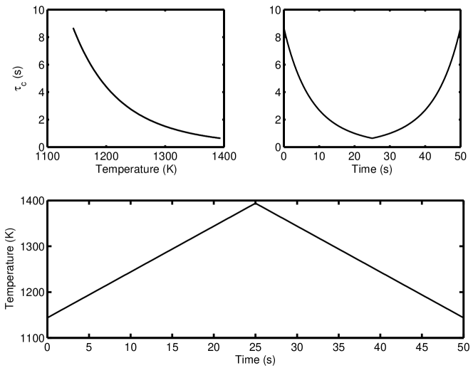
Figure 2: Temperature dependence of the characteristic time for Zircaloy-4 in the range of interest (top left) and its time-dependence for a triangular-shaped temperature pulse (bottom panel).

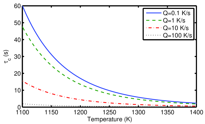
Figure 3: Characteristic time as a function of temperature and temperature rate for Zircaloy-4 according to equation (20).

The experimental results on Zircaloy-4 indicate that the starting temperature for the onset of phase transformation is temperature rate dependent [27]. This phenomenon has also been observed in other systems, e.g., ferritic-pearlitic transformation in steels [10, 11] and $\alpha\leftrightarrow\alpha+\beta$ transition of the titanium alloys [12]. In our modeling of this effect, for Zircaloy-4, we have related the onset of $\alpha\to\alpha+\beta$ transformation temperature (heating) by fitting a power law relation to the experimental data reported in [27, 43], see appendix A of [45].

As an example, for simulation of non-isothermal phase transformation, we have calculated the fraction of volume transformed during $\alpha\leftrightarrow\beta$ transition of Zircaloy-4 material by solving equation (4) employing a similar triangular temperature history shown in figure 2, but extending its tail to 75 s. The initial condition utilized for heating is $y(0)=0$, while on cooling $y(t_{f})=1$, where $t_{f}$ corresponds to the end time of heating or the beginning of cooling. The Runge-Kutta method of order 4 and 5 [46] was used to integrate equation (4). Figure 4 shows $y$ as a function of time and figure 5 depicts $y$ versus temperature. In figure 5, we have included the equilibrium curve using equation (18) and the corresponding experimental data reported in [27]. The computations on heating/cooling at the rates $\pm 10$ K/s are in agreement with the data reported in [27]. We note the asymmetry between the heating and the cooling in the computations. This is a reflection of experimental data from which the model has been adjusted to, which in turn emanates from the thermodynamic instability of the system. A more detailed comparison between experimental data and model computations, at several heating/cooling rates for zirconium alloys, is presented in [45].

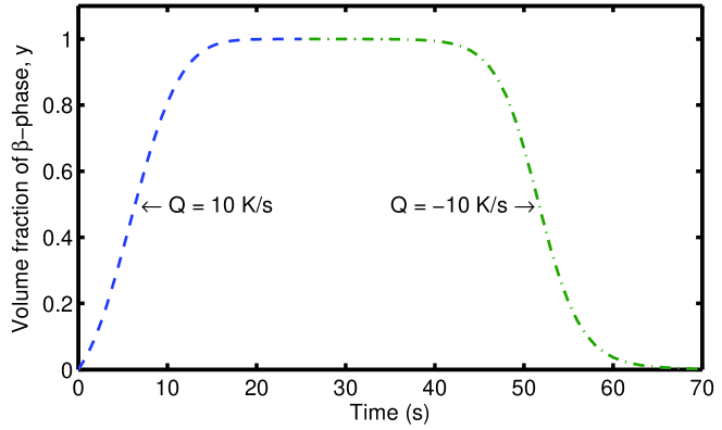
Figure 4: Calculated volume fraction of $\beta$-phase in Zircaloy-4 versus time during heating and subsequent cooling at the rates of $\pm$10 K/s, using an extended version of the temperature history shown in figure 2.

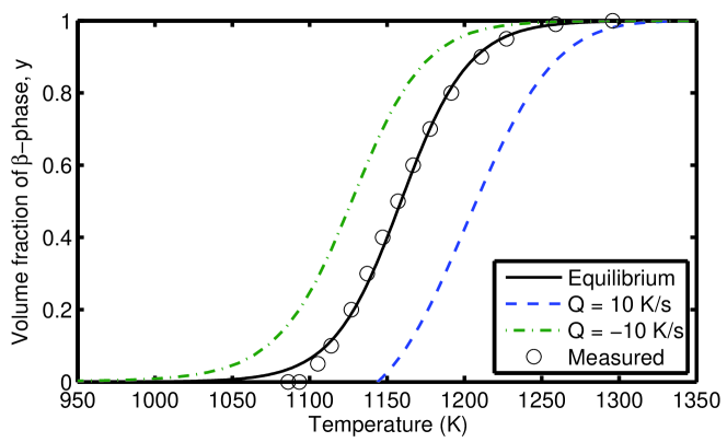
Figure 5: Calculated volume fraction of $\beta$-phase in Zircaloy-4 versus temperature during heating and subsequent cooling at the rates of $\pm$10 K/s, using an extended version of the temperature history shown in figure 2. The equilibrium curve is calculated using equation (18) and the corresponding measured data are from Forgeron et al. (2000).

4 Discussion

The method utilized here to calculate the volume fraction of the favoured phase as a function of time and temperature can be applied to any input thermal history since we solve equation (4) numerically. The question that may arise is how well this approximate equation compares with the prevailing exactly solved models in isothermal conditions.

For isothermal conditions, equation (6) yields

$$\phi=1-e^{-k(T)(t-t_{0})},$$ (21)

where $t_{0}$ is the incubation time for the onset of phase transformation. This relation is a special case of the Avrami model [7, 25] related to site saturation transformation on grain surfaces under isothermal conditions, namely

$$\phi=1-\exp\big{[}-\frac{2S}{V}v(t-t_{0})\big{]},$$ (22)

where $S/V$ is the surface area to volume ratio and $v$ the interface velocity (growth rate) of the nucleus. Moreover, as has been shown by Cahn [25], equation (22) is theoretically exact for the systems in which the nucleation rate is sufficiently rapid such that site saturation occurs early in the reaction period. Indeed, he calculated that the time at which the site saturation occurs is $t_{s}=(I_{s}v^{2})^{-1/3}$, where $I_{s}$ is the nucleation rate per unit area of the grain boundary, see A. Our considered model is related to a special case of the KJMA theory where nucleation rate is high and site saturation occurs early in reaction, see A.

A noteworthy observation in our computations, which is a reflection of experiments reported in [27], is the asymmetry in phase transformation between heating and cooling carried out at the same thermal rating, cf. figures 4 and 5. To illustrate this asymmetry, we have plotted the phase portrait of our computations in figure 6. This is a manifestation of the different initial conditions and the different paths of the two processes. In our case, we had to extend the cooling tail of the temperature history (cf. figure 2) to 950 K to complete the phase transformation, see figure 5. A thermodynamic explanation of this phenomenon even at a phenomenological level is hard for us to ascertain here; our model is purely a kinetic one.

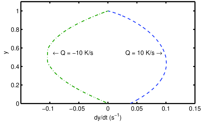
Figure 6: Calculated volume fraction $y$ of $\beta$-phase in Zircaloy-4 versus its rate $\rm dy/\rm dt$ during heating and subsequent cooling at the thermal rates of $\pm$10 K/s, using an extended version of the temperature history shown in figure 2.

The asymmetry is also true for the thermal rate dependence of the start temperature of phase transformation, cf. equations in appendix A of [45]. This type of hysteresis is ubiquitous in first-order phase transitions in solids. It is a manifestation of the solid state supercooling effect observed, e.g. in zirconium alloys, even at slow coolings [47, 48]. One reason for this behaviour is that the transformation process under non-isothermal conditions is away from equilibrium and is accompanied by dissipation of energy. The hysteresis should decrease with the decrease in transformation rate and should disappear at infinitely slow transitions. In other words, at infinitely low heating/cooling rates, the temperature variation of $y$ should collapse on the equilibrium curve. To check this, we have repeated the aforementioned computations with a thermal rate two orders of magnitude lower, i.e. at $\pm 0.1$ Ks^-1 by expanding the thermal history over 6000 s. The results are depicted in figure 7, which should be compared with figure 5. We should, nevertheless, mention that in literature, the start temperature of first order phase transition has been related to the temperature dependence of the incubation time for nucleation [49, 45].

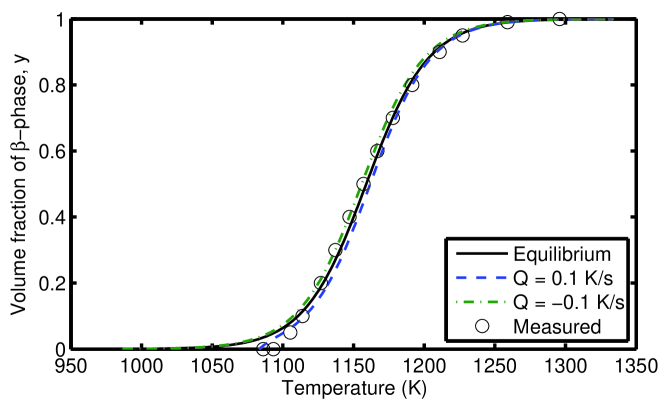
Figure 7: Calculated volume fraction of $\beta$-phase in Zircaloy-4 versus temperature during heating and subsequent cooling at the rates of $\pm 0.1$ Ks^-1, using an expanded version of the temperature history shown in figure 2. This figure should be compared with figure 5.

5 Summary and outlook

In summary, we have studied the overall phase transformation kinetics in alloys under non-isothermal conditions using a differential analysis method. The method was applied successfully to the massive phase transformation in a zirconium alloy, for which the time/temperature variations of the volume fraction of the favoured phase under heating and cooling were calculated. A trait of non-isothermal or non-equilibrium phase transitions is the dependence of the onset of the transformation temperature on heating/cooling rates. We used best-fit empirical relations to account for this effect for Zircaloy. However, we alluded to the intimate relationship between this temperature and the incubation time for nucleation. This relationship warrants further analysis and may be studied in the context of transient nucleation phenomenon.

Non-isothermal transformation kinetics is usually treated with the additivity rule, where the transient heating/cooling is treated as a series of small isothermal steps. A formulation, which embraces both additive and non-additive situations, has been suggested. Moreover, a method based on the concept of path-integral, which accounts for all the possible thermal histories to reach the final state, has been presented. The path-integral approach has the potential to provide the optimal thermal path for phase transformation to attain the desired microstructure, and thereby material’s macroscopic behavior.

Acknowledgments

We are indebted to Patrik Hermansson for valuable communications and ARM thanks Richard Warren for discussions. The work was supported in part by the Swedish Radiation Safety Authority under the contract number SKI2007/611, 200806001.

Appendix A Kolmogorov-Johnson-Mehl-Avrami model

The overall phase transformation kinetics describes the time/temperature evolution of the volume fraction of the newly transformed phase onto the stable phase. The transformations are supposed to occur by nucleation and growth mechanisms (i.e. first order transition). A mean field model was formulated and solved exactly by Kolmogorov [4], Johnson and Mehl [5], Avrami [6], Evans [50], and Jackson [51], apparently all independently. The basic assumptions of the model are : (i) the system is infinite in extent, and hence, boundary effects are neglected; (ii) nucleation is a stochastic process and on average takes place uniformly; and (iii) the growth of new phase grains ceases at the mutual points of their contact, but continues vigorously elsewhere; see ref. [52] for a recent appraisal.

Kolmogorov [4] rigorously derived a relation for the time evolution of the transformed phase $\phi$ in three dimensions. In a $d$-dimensional space, we write

$$\phi(t)=1-e^{-\phi_{e}(t)},$$ (23)

where $\phi_{e}(t)$ is the so-called extended volume fraction, expressed as

$$\phi_{e}(t)=C_{d}\int_{0}^{t}I(s)R^{d}(t,s){\rm d}s,$$ (24)

where $I(t)$ is the nucleation rate (per unit volume and time), $R(t,s)$ is the radius of the new grain (phase) at time $t$ that was nucleated at time $s$, and $C_{d}$ is a shape factor given for a hypersphere by

$$C_{d}=\frac{2\pi^{d/2}}{d\,\Gamma(d/2)},$$ (25)

with $\Gamma(\bullet)$ denoting the usual gamma function. The function $\phi_{e}(t)$ is the sum of volumes of all the transformed grains divided by the total volume of the system, supposing that the grains never cease growing and the new ones keep nucleating at the same rate in the entire material.

For $R>>R^{\ast}$, where $R^{\ast}$ is the critical radius for nucleation, $R(t,s)$ can be expressed in terms of the growth rate of the new phase as

$$R(t,s)=\int_{s}^{t}v(\tau)\rm d\tau,$$ (26)

where $v$ is the interfacial growth velocity. If now, the nucleation rate and the interfacial velocity assume anomalous power law dependencies on time, namely, $I(t)\simeq I_{0}t^{\alpha}$ and $v(t)\simeq v_{0}t^{\beta}$, then using equation (26), equation (24) can be expressed as

$$\phi_{e}(t)=\Big{(}\frac{t-t_{inc}}{\tau_{g}}\Big{)}^{m},$$ (27)

where $m$ is an overall growth exponent of the favoured phase

$$m=1+\alpha+(1+\beta)d,$$ (28)

and $\tau_{g}$ is a characteristic time for the growth of the favoured phase

$$\tau_{g}=\Bigg{[}\frac{(1+\beta)^{d+1}}{C_{d}I_{0}v_{0}^{d}\Gamma(1+d)}\Big{(}\frac{1+\alpha}{1+\beta}\Big{)}_{1+d}\Bigg{]}^{1/m},$$ (29)

with $(z)_{n}=\Gamma(z+n)/\Gamma(z)$ being a Pochhammer symbol.

Here, we have shifted the time origin as $t\Rightarrow t-t_{inc}$, according to modelling of transient nucleation in [53], where $t_{inc}$ is called the incubation time and is found to be

$$t_{inc}=t^{\ast}\ln\frac{t}{t^{\ast}}\frac{\Phi^{\ast}}{T},$$ (30)

where $t^{\ast}=R^{\ast}/v_{0}$ and $\Phi^{\ast}$ is the energy barrier for nucleation in kelvin; see also Iwamatsu’s calculations for $d=2$ [54]. To make simplifications, recall the classical nucleation theory and assume that $I_{0}$ is the steady-state nucleation rate with the form $I_{0}=I^{\ast}\exp(-\Phi^{\ast}/T)$, i.e. the number of critical nuclei per unit volume and time; e.g. see chapter 10 in [55]. Hence, according to equation (29), $\tau_{g}=\tau^{\ast}\exp(\Phi^{\ast}/mT)$. Putting $t\approx\tau_{g}$ in equation (30) gives

$$t_{inc}=t^{\ast}\frac{\Phi^{\ast}}{mT}+t^{\ast}\Big{[}\ln\frac{\Phi^{\ast}}{T}-\ln\frac{t^{\ast}}{\tau^{\ast}}\Big{]}\approx t^{\ast}\frac{\Phi^{\ast}}{mT}.$$ (31)

So, as $T$ is lowered, both $\tau_{g}$ and $t_{inc}$ are increased, albeit their unlike temperature dependence. We note that in the aforementioned formalism with $\alpha=0$, $\beta=0$ and $d=3$, with $m=4$, the frequently used expression for the KJMA model is recovered.

Cahn [25] derived relations for $\phi_{e}$ for particular cases where the new phase in a polycrystalline material nucleates on grain boundary surfaces, grain edges, or grain corners, under the condition that it grows with constant velocity. Two limiting cases corresponding to high and low nucleation rates (relative to growth rates) were found. At high temperatures, the nucleation rate is low and site saturation may not occur. If again $I\simeq I_{0}t^{\alpha}$ and assuming random nucleation on either grain surfaces, edges, corners, or interiors, Cahn found (for $d=3$)

$$\phi_{e}=8\pi\frac{\Gamma(1+\alpha)}{\Gamma(2+\alpha+d)}I_{0}v_{0}^{d}t^{m}.$$ (32)

Moreover, since $I_{0}$ would be proportional to the number of available nucleation sites, then $I_{0}\propto 1/G^{d-j}$, where $G$ is the parent phase grain size, $j=d-3$ for corner, $j=d-2$ for edge, $j=d-1$ for surface, and $j=d$ for intragranular nucleation. Equation (32), except for a numerical factor and a shift in time origin, is close to the general equation (27).

For high nucleation rates, site saturation occurs early in the reaction and $\phi_{e}$ becomes independent of nucleation rate. The reaction is completed when $t=0.5G/v$ [25]

$$\phi_{e}=C_{n}\rho_{n}(vt)^{n}.$$ (33)

Here, $n=1$, 2, 3 correspond respectively to site saturation on grain surfaces, edges and corners; and $\rho_{n}$ denotes the ratio of the respective surface area, grain-edge length and grain corner number per unit volume; note that $\phi_{e}$ is independent of nucleation rate and is driven by the growth rate. If we put $v(t)\simeq v_{0}t^{\beta}$, then $\phi_{e}\simeq C_{n}\rho_{n}v_{0}^{n}t^{n(1+\beta)}\equiv k_{n}t^{n(1+\beta)}$.

Thus, for $n=1$ (grain boundary site saturation) and $\beta=0$ equation (23) can be written as

$$\phi=1-e^{-k_{1}t},$$ (34)

where $k_{1}=C_{1}\rho_{1}v_{0}=2(S/V)v_{0}$, which except a shift in the time origin, is exactly the same as equations (21)-(22), and is equivalent to the model we have used in our analysis.

It is worthwhile to mention that Ham [56] obtained a similar kind of relation as (34) for diffusion-limited precipitation of second phase in a crystalline. In Ham’s model, one may imagine that a polycrystalline consists of an array of parallel cylinders, in which the solute atoms precipitate on cylinders’ surfaces. For this model, the precipitated fraction of excess solute $w$ can be calculated as a function of time $t$ fairly accurately by the simple relationship

$$w\cong 1-e^{-t/\tau_{0}},$$ (35)

where $\tau_{0}=\ell^{2}/(\alpha_{0}^{2}D)$, $\ell$ is the inter-precipitate distance, $\alpha_{0}$ the lowest eigenvalue of the prevailing diffusion equation, and $D$ is the solute diffusivity. Hence, the theoretical basis of the model used for calculations of phase transformation kinetics in this paper may be attributed to a special case of the KJMA formulation, or diffusion-limited phase transformation on surfaces.

References

References

- [1] J. D. Gunton, M. San Miguel, and P. S. Sahni. The dynamics of first-order phase transition. In C. Domb and J. L. Lebowitz, editors, Phase Transitions and Critical Phenomena, volume 8, chapter 3, pages 267–479. Academic Press, London, England, 1983.
- [2] J. S. Langer. In C. Godrèche, editor, Solids Far from Equilibrium, chapter 3, pages 297–363. Cambridge University Press, Cambridge, UK, 1992.
- [3] D.A. Porter and K.E. Easterling. Phase Transformations in Metals and Alloys. Chapman Hall, London, UK, 1981. Chapter 5.
- [4] A. N. Kolmogorov. Statistical theory of metal crystallization. Izv. Akad. Nauk SSSR, 1:355–359, 1937. in Russian.
- [5] W. A. Johnson and R. F. Mehl. Reaction kinetics in processes of nucleation and growth. Trans. of AIME, 135:416–442, 1939.
- [6] M. Avrami. Kinetics of phase change I: General theory. J. Chem. Phys., 7:1103–1112, 1939.
- [7] M. Avrami. Kinetics of phase change II: Transformation-time relations for random distribution of nuclei. J. Chem. Phys., 8:212–224, 1940.
- [8] J. W. Cahn. Transformation kinetics during continuous cooling. Acta Met., 4:572–575, 1956.
- [9] E. B. Hawbolt, B. Chau, and J. K. Brimacombe. Kinetics of austenite-pearlite transformation in eutectoid carbon steel. Metall. Trans. A, 14A:1803–1815, 1983.
- [10] J. B. Leblond and J. Devaux. A new kinetic model for anisothermal metallurgical transformations in steels including the effect of austenite grain size. Acta Met., 32:137–146, 1984.
- [11] M. Umemoto, K. Horiuchi, and I. Tamura. Pearlite transformation during continuous cooling and its relation to isothermal transformation. Trans. ISIJ, 23:690–695, 1983.
- [12] B. K. Damkroger and G. R. Edwards. Continuous cooling transformation kinetics in alpha-beta titanium alloys. In M.P. Anderson, editor, Simulation and Theory of Evolving Microstructures, pages 129–150. The Minerals, Metals Material Society, 1990.
- [13] S. Malinov, Z. Guo, W. Sha, and A. Wilson. Differential scanning calorimetry study and computer modeling of phase ransformation in a Ti-6Al-4V alloy. Metall. Mater. Trans. A, 32A:879–887, 2001.
- [14] I. A. Wierszyłłowski. The effect of the thermal path to reach isothermal temperature on transformation kinetics. Metall. Trans. A, 22A:993–999, 1991.
- [15] M. Lusk and H-J Jou. On the rule of additivity in phase transformation kinetics. Metall. Mater. Trans. A, 28A:287–291, 1997.
- [16] Y. T. Zhu, T C. Lowe, and R. J. Asaro. Assessment of the theoretical basis of the rule of additivity of the nucleation incubation time during continuous cooling. J. Appl. Phys., 82:1129–1137, 1997.
- [17] T. Réti and I. Felde. A non-linear extension of additivity rule. Comput. Mater. Sci., 15:466–482, 1999.
- [18] A. T. W. Kempen, F. Sommer, and E. J. Mittemeijer. Determination and interpretation of isothermal and non-isothermal transformation kinetics; the effective activation energies in terms of nucleation and growth. J. Mater. Sci., 37:1321–1332, 2002.
- [19] E. J. Mittemeijer and F. Sommer. Solid state phase transformation kinetics: a modular transformation model. Z. Metallkd., 93:352–361, 2002.
- [20] F. Liu, F. Sommer, and E. J. Mittemeijer. An analytical model for isothermal and isochronal transformation kinetics. J. Mater. Sci., 39:1621–1634, 2004.
- [21] F. Liu, F. Sommer, and E. J. Mittemeijer. Determination of nucleation and growth mechanisms of the crystallization of amorphous alloys; application to calorimetric data. Acta Mater., 52:3207–3216, 2004.
- [22] F. Liu, F. Sommer, C. Boss, and E. J. Mittemeijer. Analysis of solid state phase transformation kinetics: models and recipes. Intern. Mater. Rev., 52:193–212, 2007.
- [23] J. Farjas and P. Roura. Modification of the Kolmogorov-Johnson-Mehl-Avrami rate equation for non-isothermal experiments and its analytical solutions. Acta Mater., 54:5573–5579, 2006.
- [24] K. R. Elder, J. D. Gunton, and M. Grant. Nonisothermal eutectic crystallization. Phys. Rev. B, 54:6476–6484, 1996.
- [25] J. W. Cahn. The kinetics of grain boundary nucleated reactions. Acta Met., 4:449–459, 1956.
- [26] A. R. Massih, T. Andersson, P. Witt, M. Dahlbäck, and M. Limbäck. The effect of quenching rate on the -to- phase transformation structure in zirconium alloy. J. Nucl. Mater., 322:138–151, 2003.
- [27] T. Forgeron, J. C. Brachet, F. Barcelo, A. Castaing, J. Hivroz, J. P. Mardon, and C. Bernaudat. Experiment and modeling of advanced fuel rod cladding under LOCA conditions: alpha-beta phase kinetics and EDGAR methodology. In G. P. Sabol and G. D. Moan, editors, Zirconium in Nuclear Industry: Twelfth International Symposium, volume ASTM STP 1345, pages 256–278, West Conshohocken, PA, USA, 2000. American Society for Testing and Materials.
- [28] P. Hermansson. Personal communication, 2008.
- [29] H. Mori. Transport, collective motion and Brownian motion. Prog. Theor. Phys., 33:423–455, 1965.
- [30] D. Forster. Hydrodynamic Fluctuations, Broken Symmetry, and Correlation Functions. W. A. Benjamin, Inc., Reading, MA, USA, 1975.
- [31] E. J. Mittemeijer. Review: Analysis of kinetics of phase transformation. J. Mater. Sci., 27:3977–3987, 1992.
- [32] C. Lemaignan and A. T. Motta. Zirconium alloys in nuclear applications. In R. W. Cahn, P. Haasen, and E. J. Kramer, editors, Nuclear Materials, volume 10B of Material Science and Technology, chapter 7. VCH, Weinheim, Germany, 1994. Volume editor B.R.T. Frost.
- [33] A. Miquet, D. Charquet, and C. H. Allibert. Solid state phase equilibria of Zircaloy-4 in the temperature range 750-1050∘C. J. Nucl. Mater., 105:132–141, 1982.
- [34] N. V. Bangaru, R. A. Busch, and J. H. Schemel. Effects of beta quenching on the microstructure and corrosion of Zircaloys. In R.B. Adamson and L.F.P. van Swam, editors, Zirconium in Nuclear Industry: Seventh International Symposium, volume ASTM STP 939, pages 341–363, Philadelphia, USA, 1987. American Society for Testing and Materials.
- [35] G. Ökvist and K. Källström. The effect of zirconium carbide on the transformation structure in Zircaloy. J. Nucl. Mater., 35:316–321, 1970.
- [36] D. Charquet and E. Alheritier. Influence of the impurities and temperature on the microstructure of Zircaloy-2 and Zircaloy-4 after transformation. In R.B. Adamson and L.F.P. van Swam, editors, Zirconium in Nuclear Industry: Seventh International Symposium, volume ASTM STP 939, pages 284–291, Philadelphia, USA, 1987. American Society for Testing and Materials.
- [37] R. A. Holt. The beta to alpha phase transformation in Zircaloy-4. J. Nucl. Mater., 35:322–334, 1970.
- [38] R. A. Holt. Comments on the beta to alpha phase transformation in Zircaloy-4. J. Nucl. Mater., 47:262–264, 1973.
- [39] O. T. Woo and K. Tangri. Transformation characteristics of rapidly heated and quenched Zircaloy-4-oxygen alloys. J. Nucl. Mater., 79:82–94, 1979.
- [40] C. E. L. Hunt and E. M. Schulson. Recrystallization of Zircaloy-4 during transient heating. J. Nucl. Mater., 92:184–190, 1980.
- [41] M. Corchia and F. Righini. Kinetic aspects of the phase transformation in Zircaloy-2. J. Nucl. Mater., 97:137–148, 1981.
- [42] J. S. Yoo and I. S. Kim. Effect of () heat treatment on the mechanical properties of Zircaloy-4. J. Nucl. Mater., 185:87–95, 1991.
- [43] J. C. Brachet, L. Portier, and T. Forgeron. Influence of hydrogen content on phase transformation temperatures and on the thermal-mechanical behavior of Zy-4, M4, and M5TM (ZrNbO) alloys during the first phase of LOCA tranient. In G. D. Moan and P. Rudling, editors, Zirconium in Nuclear Industry: Thirteenth International Symposium, volume ASTM STP 1423, pages 673–701, West Conshohocken, PA, USA, 2002. American Society for Testing and Materials.
- [44] A. Miquet, D. Charquet, C. Michaut, and C. H. Allibert. Effect of Cr, Sn and O contents on the solid state phase boundary temperature of Zircaloy-4. J. Nucl. Mater., 105:142–148, 1982.
- [45] A. R. Massih. Transformation kinetics of zirconium alloys under non-isothermal conditions. J. Nucl. Mater., 384:330–335, 2009.
- [46] A. Quarteroni and F. Saleri. Scientific Computing with MATLAB. Springer, Berlin, Germany, 2003.
- [47] A. Miquet, D. Charquet, and C. H. Allibert. Solid-state phase equilibria of Zircaloy-4 in the temperature range 750-1050∘c. J. Nucl. Mater., 105:132–141, 1982.
- [48] M. Canay, C. A. Danon, and D. Arias. Phase transition temperature in the Zr-rich corner of Zr-Nb-Sn-Fe alloys. J. Nucl. Mater., 280:365–371, 2000.
- [49] Y. T. Zhu and J. H. Devletian. Determination of equilibrium solid-phase transition temperature using DTA. Metall. Trans. A, 22A:1993–1998, 1991.
- [50] U. R. Evans. The laws of expanding circles and spheres in relations to the lateral growth of surface films and the grain-size of metals. Trans. Faraday Soc., 41:365–374, 1945.
- [51] J. L. Jackson. Dynamics of expanding inhibitory fields. Science, 183:444–446, 1974.
- [52] A. A. Burbelko, E. Fras, and W. Kapturkiewicz. About Kolmogorov’s statistical theory of phase transformation. Mater. Sci. Eng. A, 413-414:429–434, 2005.
- [53] V. A. Shneidman and M. C. Weinberg. The effects of transient nucleation on size-dependent growth rate on phase transformation kinetics. J. Non-Cryst. Solids, 160:89–98, 1993.
- [54] M. Iwamatsu. Direct numerical simulation of homogeneous nucleation and growth in a phase-field model using cell dynamics method. J. Chem. Phys., 128:084504, 2008.
- [55] J. W. Christian. The Theory of Transformations in Metals and Alloys. Pergamon, Amsterdam, 2002.
- [56] F. S. Ham. Stress-assisted precipitation on dislocations. J. Appl. Phys., 30(6):915–926, 1959.